2.5-dimensional topological superconductivity in twisted superconducting flakes

Introduction
The realization of twisted two-dimensional (2-D) moiré materials has led to several discoveries of novel correlated electronic phases1,2,3. The field has advanced from twisted bilayer graphene (TBG) to new discoveries in hBN substrate-aligned TBG3 and twisted graphene multilayers4,5,6,7,8, magnetic moiré structures9, and twisted or stacked transition metal dichalgonides (TMDs)10,11. In particular, TMDs have been instrumental in observing anomalous topological phases such as a quantum anomalous Hall effect likely due to orbital ferromagnetism in heterostructures12, and (fractional) Chern insulators in twisted bilayers13,14,15. Recently, the twist paradigm has been extended to 2-D nodal superconducting materials, leading to proposals that realize chiral topological superconductivity16,17 and spontaneous time-reversal symmetry breaking16,18,19,20,21,22.
The unusual properties of twisted bilayers have motivated proposals for multilayer structures23,24, going all the way to three dimensions (3-D)25 to realize new electronic states, including topological ones. Theoretically, layered chiral topological systems can realize new types of behavior including edge sheaths for integer quantum Hall multilayers26,27. Moreover, their extension to interacting systems have been predicted to form new types of topological ordered phases in 3-D27,28,29,30.
Another approach to extend the possible phenomena of 2-D materials is to consider twisted flakes of finite thickness. Remarkably, recent experiments have demonstrated that even a single layer of graphene twisted on top of a finite-thickness graphite flake can modify the electronic structure of the whole flake31,32. Single layer twists represent a simple but novel route to realize effective “2.5-D” heterostructures that truly lie in between two and three dimensional behavior.
For twisted superconducting platforms18,33,34, there is also a practical motivation to study multilayers. While nodal superconductivity in individual bi- and mono-layers has been achieved35,36, realizing twisted bilayers remains a challenge. Instead, experiments focused on the interfaces between finite-thickness flakes18,33,34. Such a setup differs from the proposed twisted multilayer structures23,24, where the twist angle between each pair of layers has to be controlled. Prior numerical results on twisted flakes with spontaneously broken time-reversal symmetry around 45∘37 indicate that the nodal gaps fall off rapidly with layer thickness. However, the character of the topological states that can be induced by current at all twist angles17 has not been determined.
In this work, we consider the possibility of inducing topological superconductivity in a twisted multilayer flake of nodal superconductors. Focusing on the case of a N-layer flake with the top layer twisted (Fig. 1a, b), we demonstrate that the twisted interface induces topological superconductivity in the whole flake with an interlayer supercurrent. While the topological gap is reduced in flakes as ({mathcal{O}}(1/N)), we identify experimentally accessible observables (density of states and thermal Hall effect) that are thickness-independent. Unexpectedly, we find that increasing the current flowing through the stack leads to a sequence of topological transitions, reconstructing the quasiparticle spectrum of the whole flake. In every transition, new Dirac points are generated, with their total number growing up to ({mathcal{O}}({N}^{2})). In the bulk limit, this reflects the emergence of a Bogoliubov Fermi surface in the current-driven nodal superconductor38,39,40. For a finite thickness flake, this allows the Chern number to increase up to ({mathcal{O}}({N}^{2})) (Fig. 1c), beyond the expectation from N independent layers of topological superconductors, opening the path to intermediate, “2.5-D” topological superconductivity.

a Illustration of the N-layer flake for θ1,2 ≈ 53∘. Inset: single moiré unit cell. b Momentum-space illustration for N = 2. Shown are the Fermi surfaces of each layer with a ({d}_{{x}^{2}-{y}^{2}}) singlet order parameter, with its sign marked by color and quasiparticle nodes highlighted in orange. Combination of momentum-space rotation and interlayer supercurrent IJ produces a Nambu-space rotation of a d-wave order parameter to a d + id topological one. c Phase diagram of N-layered systems for varying current and twist angles θ < θMA. Shown are the predicted net Chern numbers, C(φ), as a function of normalized Josephson current ((frac{{I}_{J}(varphi )}{{I}_{c}})). For N ≤ 5, C grows linearly with N and is independent of IJ, but for N ≥ 6, topological phase transitions can occur increasing C to values up to ({mathcal{O}}({N}^{2})) for N ≫ 1.
The paper is organized as follows. We present two models: a microscopic model of a moiré superlattice and a low energy continuum model of a single valley of N Dirac nodes in Sec. II A. We then explore two setups for the application of an interlayer supercurrent. First, we consider supercurrent applied between the top two layers only (Sec. II B). Small and large twist angle limits are anlyzed to understand the evolution of topological superconductivity with N. In the second setup, supercurrent flows though the entire stack of layers (Sec. II C). We demonstrate the appearance of new pairs of nodes due to the current in Sec. II C and 2.5-D topological superconductivity which manifests as topological transitions driven by the current in Sec. II D. With the results from both the lattice and continuum models complete, we compare their results in Sec. II E. Experimental probes are then introduced in Sec. II F: density of states and thermal Hall effect which provide signatures of topological superconductivity predicted in our models. Using the thermal Hall effect, we highlight how the topological phase transitions from new nodes generated by a current through the stack can be probed in Sec. II F. We end with Sec. III to summarize the results and comment on the emergence of 2.5-D phenomena in the twisted superconducting flakes.
Results
Models
We utilize two models to approach the N layered system: a real-space tight-binding model of the twisted multilayer16 and an approximate momentum-space model around the Dirac gap nodes17. In both cases, we assume that interlayer tunneling is weak compared to the superconducting gap maximum41, allowing us to neglect the corrections to the self-consistency equation due to tunneling19 and treat the order parameter as fixed. We use the first model to exactly include the effects of moiré reconstruction of the bands and to study the topological edge modes, but limit its use to large commensurate twist angles (theta, >, {theta }_{MA}=frac{2{t}_{z}}{{v}_{Delta }{K}_{N}}), where tz is the magnitude of the interlayer tunneling, vΔ is the velocity of the order parameter around the node, and KN is the position of the untwisted Dirac node of a single nodal superconductor layer. In this case, the moiré unit cell is not too large, and we consider moderate values of N. The continuum model, on the other hand, allows us to study effects of arbitrary N and twist angles analytically. This allows us to compare the results of two models at large twist angles where we find good agreement in the overlapping regimes of applicability.
To model the system at the microscopic lattice level, we use a tight-binding approach. In absence of interlayer tunneling, the Hamiltonian takes the form:
where n, σ and i, j are the layer, spin and site indices, respectively, and 〈i, j〉 is a sum over nearest neighboring sites on the square lattice. t and μ are the single-electron hopping and chemical potential, while Δij is the d-wave SC order parameter
The square lattice sites for n = 1 are rotated by an angle θ (see Fig. 1a). The single-electron hopping between the layers is described by:
where ({g}_{ij}={g}_{0}{e}^{-({r}_{ij}-d)/rho }), g0 being the overall tunneling magnitude and ({r}_{ij}=sqrt{{d}_{ij}^{2}+{d}^{2}}) with dij the in-plane distance between sites and d is the interlayer distance along the z-axis. We do not take the dependence of tunneling on the twist angle due to orbital structure, relevant for cuprates22, into account. Inclusion of these effects would be important for studying quantitative behavior of system’s properties for different twist values as it sets the overall scale, e.g. the magnitude of the topological gap; however these effects are system-dependent and need to be studied on a case by case basis. Here, we will instead focus on qualitative effects of increasing N, leaving quantitative studies for particular systems for future work. We note however, that at low twist angles relevant for the continuum model introduced below, the dependence of nodal tunneling on angle is weak (propto cos (2theta )) and can be rigorously neglected. We use parameters similar to previous studies: Δ = 40 meV16, t = − 126 meV and μ = 15 meV20,41, ρ = 2.11Å and d = 12Å is the interlayer separation16. We also restrict our numerical analysis to twist angles where the system is strictly periodic: ({theta }_{p,q}=2arctan left(frac{p}{q}right)), where (p,qin {mathbb{N}}). We implement the twist by rotating square lattices of the top and remaining N − 1 layers in opposite directions by θp,q/2.
Finally, we consider two setups for applying supercurrent (which has been shown to induce topology in bilayers17,19): current applied through the entire stack (Fig. 2a) and current applied between the top two layers only (Fig. 2b). The current IJ(θ) between two neighboring layers in a flake is related to the phases of the order parameters by the Josephson relation20,42,43:
where Ic(θ) is the critical current which depends on the twist angle between the two layers, and φn is the phase of the order parameter where n = 1, 2 is the layer index. In experiments on twisted flakes of BSCCO18, the critical current was found to follow the expected d-wave form ({I}_{c}(theta )approx {I}_{c}cos (2theta ),) consistent with predictions for inhomogeneous tunneling20. Therefore, the critical current between the top and next layer is reduced with respect to the rest of the stack. A constant Josephson current then corresponds to φn = nφ, for layer n with n ≠ 1 and φ1 = 2φ − φc for the top layer (n = 1) where ({varphi }_{c}=arcsin (frac{sin varphi }{cos (2{theta }_{p,q})})).
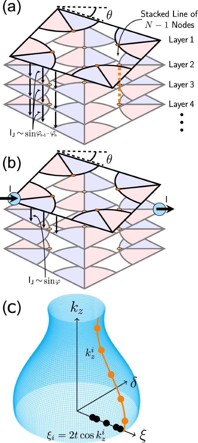
a Illustration of a N layered flake of ({d}_{{x}^{2}-{y}^{2}}) superconductors with a supercurrent IJ with current applied through the stack. b displays the same setup except current is fed in and picked up in the top two layers. c Emergence of Dirac nodes in N-layer flake without supercurrent from 3-D (N → ∞) Fermi surface in the space of ξ (Eq. (4)), δ (Eq. (5)), and kz. A line node appears along kz in 3-D highlighted by the orange curve. For a finite N, kz becomes quantized (see Eq. (9)) illustrated by the orange points along the curve. Because of the quantization, N Dirac nodes are introduced at corresponding values ({xi }_{i}=2{t}_{z}cos {k}_{z}^{i}) illustrated by the black points along ξ.
To access small twist angles and arbitrary N, we construct a low energy continuum model of the system depicted in detail for N = 2 in Fig. 1b and generalize it to a N layer flake shown in Fig. 2a, b. We focus on the case of singlet superconductors, with extensions to triplet being discussed in ref. 19. Each layer of the system is characterized by a single-particle dispersion ε(k)τ3 and a superconducting order parameter Δ(k)τ1 where τi represent matrices in Gor’kov-Nambu space.
Near the nodes, where ε(KN) = 0, Δ(KN) = 0, we expand to linear order and define variables19,
and
where vF and vΔ are the velocities of the normal dispersion and the order parameter, respectively. Since ({{bf{v}}}_{F}={v}_{F}{hat{k}}_{parallel }) and ({{bf{v}}}_{Delta }={v}_{Delta }{hat{k}}_{perp }) where ({hat{k}}_{parallel }) is the direction parallel to KN and ({hat{k}}_{perp }) the direction perpendicular, ξ and δ can be treated as an orthogonal coordinate system local to KN. The interlayer tunneling can be approximated by a constant term tzτ319. The effect of the twist of the top layer in the vicinity of KN is to shift the top layer momentum by Q = − θ[KN × z]. We further consider the case of a circularly symmetric dispersion ε(K); for θ ≪ θMA non-circular corrections are negligible, while at large twists their effect does not alter the qualitative behavior in twisted bilayers19. Therefore, the twist contributes a term δ0τ1 for the top layer, where δ0 = vΔ ⋅ Q. We also assume θ ≪ 1, such that the θ -dependence of Ic in Eq. (3) (leading to corrections of the order O(θ2)) can be neglected. Under that assumption, uniform supercurrent along the stack corresponds to Δn(k) → Δn(k)eiφn where n is the layer index. The resulting Hamiltonian in the vicinity of a single node within each layer takes the form
where ({Phi }_{n}^{dagger }=({c}_{uparrow ,n}^{dagger },{c}_{downarrow ,n})) are the Nambu spinors for layer n, tz is the tunneling strength at the Dirac node17,19, and δn,1 is the Kronecker delta acting in layer space.
Current through the top interface: d+
id proximity effect
We begin with a simplified version of the problem, Eq. (6), where phase difference is nonzero between the top two layers only (see Fig. 2b). This corresponds to the current being applied only between the top two layers being fed in from the flake’s side, as in ref. 18. Assuming that the in-plane critical current is much larger than the c-axis one, the in-plane phase gradient can be neglected. A similar situation is expected to arise at twist angles close to 45∘ with the current driven through the whole flake. Due to the suppression of the critical current at the top interface as implied by Eq. (3), the phase differences for the other interfaces are strongly reduced ((varphi =arcsin (sin {varphi }_{c}cos 2theta )to 0) for a fixed φc). The effect of the supercurrent reduces thus to Δ1(k) → Δ1(k)e−iφ.
We break the Hamiltonian down into three parts
where each term is expressed as:
H0(k) describes the system without twist or current, while the remaining part is split into ({H}_{{rm{cur}}}^{1}({k}_{perp },varphi )) which describes the effect of current between the top two layers and Htwist(φ) for the twist of the n = 1 layer. In this section we take phase at the top layer to be − φ to keep the phase difference between 2 and 1 equal to φ. We first consider the case of low twist angles θ ≪ θMA (δ0 ≪ t), where twist can be treated perturbatively. Moreover, below we show that the effect of ({H}_{{rm{cur}}}^{1}({k}_{perp },varphi )) is negligible in this limit.
The eigenstates of H0(k) (system in the absence of supercurrent and twist) are superpositions of plane waves along z, with open boundary conditions at n = 1 and n = N. The latter are equivalent to adding two additional layers n = 0, N + 1 and requiring the eigenstates of the system to vanish at n = 0, N + 1. The resulting eigenstates are:
where ({psi }_{{bf{k}},n}^{dagger }) is a spinor composed of ({psi }_{{bf{k}},n}^{dagger }={Phi }_{{bf{k}},n}^{dagger }-{Phi }_{-{bf{k}},n}^{dagger }) and ({k}_{z}^{i}=frac{ipi }{N+1}), i = 1, 2, …, N. In this basis, the Hamiltonian H0(k) takes the form:
with energies given by
Figure 2b represents the model as seen in layer space and transformed into kz in Fig. 2c. In the N → ∞ limit, the zero-energy manifold takes the form of a nodal line along the z-axis: (xi =2{t}_{z}cos {k}_{z}), δ = 0, where kz ∈ [0, π]. On the other hand, for finite N the boundary conditions restrict kz to N discrete values on this nodal line resulting in a discrete set of zero-energy (Dirac) points at ({xi }_{i}=2{t}_{z}cos {k}_{z}^{i}), δ = 0 (see Fig. 2c).
Projecting Htwist(φ) onto the eigenstates H0(k) (Eq. (9)), we find terms acting within a single ({k}_{z}^{i}) subspace that couple the two zero-energy states of the Dirac cones as well as those coupling different ({k}_{z}^{i}). For the latter, applying second-order perturbation theory yields O(1) terms of order (frac{{[{delta }_{0}sin (varphi )]}^{2}}{2{t}_{z}}) and O(N) terms of order (frac{1}{N}frac{{[{delta }_{0}sin (varphi )]}^{2}}{2{t}_{z}}). We neglect these term by applying ({delta }_{0}sin varphi, ll, t), which can be fulfilled for small enough twist angle and/or current. As a result, we get the effective Hamiltonian:
where we omitted the shift of δ due to the τ1 term in Htwist and the corrections due to ({H}_{cur}^{1}) are small on the order of O(1/N2) for relevant values of δ ~ δ0/N. We therefore find that the presence of the id component in the top layer “proximitizes” the whole flake, opening gaps at all Dirac nodes each with a mass given in Eq. (12). The value of the topological gap is suppressed with N and vanishes in the N → ∞ limit, highlighting that this effect is absent in bulk 3-D materials. The power-law-like suppression of the gap, can be qualitatively attributed to the gapless character of the Dirac quasiparticles in the flake, whereas for a gapped superconductor an exponential suppression of the idxy component is expected.
Importantly, the chirality of all the resulting gapped Dirac nodes is the same, which for a two band continuum model corresponds to a Chern number of every point to be ± 1/244, so that they add up to (pm frac{N}{2}). Furthermore, this model considers only the Dirac nodes arising in the vicinity of one original Dirac node of the 2-D superconductor, but the total Chern number will depend on the sum of all nodes in the Brillouin zone. In fact, symmetry-related nodes in the Brillouin zone will also have the same Chern number17, resulting in
where Nsym is to total number of symmetry-related nodes in the Brillouin zone. For instance, Nsym = 4 for the case of d-wave (4 nodes related by C4 symmetry). This prediction is consistent with N layers being “proximitized” by the topological superconductivity emerging at the interface. Experimentally, this leads to an increase of the thermal Hall response of the system at low temperature discussed in detail in Sec. II F.
Another important characteristic of a chiral topological superconductor is the value of the gap opening at a Dirac node. Eq. (12) demonstrates that the gap values are different at different nodes, so that the system is described by a distribution of topological gaps, rather than a single one. For N ≫ 1, the topological gaps for nodes with i ≪ N (or ∣N − i∣ ≪ N) scale as (m({k}_{z}^{i},varphi )propto {mathcal{O}}({N}^{-3})). On the other hand, the typical gap scales as ({langle m({k}_{z}^{i},varphi )rangle }_{{rm{typ}}} sim {mathcal{O}}({N}^{-1})), which dominates the average gap value for N ≫ 1 given by (langle m({k}_{z}^{i},varphi )rangle =frac{{delta }_{0}sin varphi }{N+1}). Therefore, while the proximity-induced topological gap is reduced with the flake thickness, the reduction is only power-law like due to the gapless character of the unperturbed system. Combined with an increase in Chern number, this leads to robust experimental signatures of topology in flakes, discussed in Sec. II F.
We now consider the opposite case θ ≫ θMA. The model Eq. (7) can be still used in this regime provided that θMA ≪ 1. In this case, the tunneling between the top two layers can be treated perturbatively, as the respective Dirac points are far apart for δ0 ≫ tz. The Hamiltonian of the top layer is given by
and for the remaining N − 1 layers, we will utilize the Hamiltonian Eq. (10), with ({k}_{z}^{i}to {k}_{z}^{{i}^{{prime} }}=frac{pi {i}^{{prime} }}{N}). We now introduce a tunneling term between layer 1 and layer 2
Applying second order perturbation theory to the zero energy eigenstates produces the following correction to the Hamiltonian
for i = 2, …, N. The corresponding Dirac mass term is then
which scales with N in the same way as for the low twist case above.
The Dirac point of the top layer, however is at ξ = 0, δ = − δ0 initially, allowing one to apply the limit δ0 ≫ tz such that second order perturbation theory simply couples layers 1 and 2, yielding (-frac{{t}_{z}^{2}}{{delta }_{0}}{tau }_{1}) for the top layer. Combining this term with Eq. (14) and a unitary transformation ({Phi }_{1}to {e}^{-ivarphi /2{tau }_{3}}{Phi }_{1}) one obtains an effective Dirac Hamiltonian with the same chirality and a gap
that is independent of N. This leads to N-independent spectral signatures of topological superconductivity discussed in Sec. II F.
We mention briefly that this approach is straightforward to generalize for a system of two twisted flakes with M and N layers. Carrying out the previous analysis shows that the masses will be (frac{2{t}_{z}^{2}{sin }^{2}{k}_{z}^{i,N}sin varphi }{{delta }_{0}(N+1)}{tau }_{2}) for the nodes in N layers and (frac{2{t}_{z}^{2}{sin }^{2}{k}_{z}^{i,M}sin varphi }{{delta }_{0}(M+1)}{tau }_{2}) for the nodes in M layers, where ({k}_{z}^{i,M(N)}=frac{ipi }{M(N)+1}). Thus, the proximity effect arising from the twisted interface should persist to a twist between M and N layers though each gap is reduced by the respective thickness of each flake. For M = 1, N → N − 1 we recover the results above.
Current through whole flake: generation of Dirac points by current
We now move onto the case with finite current applied through the whole system (Fig. 2a and Eq. (19)).
Following a similar approach as in Sec. II B, we break Eq. (19) in three parts H(k, φ) = H0(k) + Hcur(k⊥, φ) + Htwist(φ), such that H0 and Htwist are the same as in Eq. (8), while Hcur is:
Projecting Hcur(k⊥, φ) + Htwist(φ) onto the basis of Eq. (10) for θ ≪ θMA case (see Supplementary Note 1A for θ ≫ θMA) we find a modified effective Hamiltonian:
For φ ≪ 1/N, the low-energy spectrum takes the form of N gapped Dirac nodes at δ = 0. In contrast to the case with current between two top layers, the magnitude of the gap is larger in this regime by a factor of N.
On increasing φ, we find that the Dirac structure at δ = 0 is modified at specific values of φ:
In case (i) above, the Dirac velocity becomes zero along the k⊥(δ) direction. The chirality of the node changes after on further increasing φ; however, as discussed below, additional gapped Dirac points will appear at δ ≠ 0. For case (ii), once φ = φj the gap for the δ = 0 Dirac nodes close and reopen afterwards, with a change of chirality.
The above suggests that to understand the topological properties of the full system, we need to consider the possibility of Dirac nodes forming at δ ≠ 0. We will demonstrate now that this occurs even without the twist. To do that, we find the zero-energy eigenstates of H0(k) + Hcur(k⊥, φ), i.e. consider a single flake without twist. By applying a transformation ({c}_{n}^{dagger }to {e}^{-ivarphi n/2}{c}_{n}^{dagger }), H0(k) + Hcur(k⊥, φ) can be brought to the form:
Away from the boundaries, the eigenstates of Eq. (23) are superpositions of plane waves (leftvert {k}_{z}rightrangle =frac{1}{sqrt{N}}mathop{sum }nolimits_{n = 1}^{N}{e}^{i{k}_{z}n}(a({k}_{z})leftvert n,uparrow rightrangle +b({k}_{z})leftvert n,downarrow rightrangle )) where ↑/↓ signify τ3 eigenvectors. These states satisfy
The energy eigenvalues of Eq. (24) are given by:
For each value of ξ < 2tz we find 4 zero-energy eigenstates with kz = ± k±, where k± are determined by
For the bulk 3-D case (N → ∞), where kz can vary continuously, the zero-energy states Eq. (26) form a closed 2-D surface (see Fig. 3). We now introduce open boundary conditions as in the case leading to Eq. (9), which yields a quantization condition ({k}_{z}^{i}=frac{ipi }{N+1}) (see additional discussion in Supplementary Note 1 B). The boundary conditions constitute 4 equations and thus a solution exists if there are 4 states with the same energy for a given ξ, δ. In the case of zero-energy states, the ({k}_{z}^{i}) quantization selects discrete “rings” in ξ, δ space (see Fig. 3) which are doubled by the particle-hole symmetry of the Hamiltonian from Eq. (24). Four zero-energy solutions at the same ξ, δ thus occur only when the projections of two rings on the (ξ, δ)-plane intersect (see Fig. 3a). This corresponds to quantizing the momenta in Eq. (26) as ({k}_{+}^{n}={k}_{z}^{i}+{k}_{delta }=frac{npi }{N+1}) and ({k}_{-}^{m}={k}_{z}^{i}-{k}_{delta }=frac{mpi }{N+1}) with arbitrary integer 1 ≤ n, m ≤ N. These conditions require quantization of kδ as ({k}_{delta }^{j}in {frac{jpi }{N+1}| 1le jle N}). As explored in the Supplementary Note 1A, the quantization condition for k± implies that the new Dirac nodes exist when:
where ({k}_{delta }^{j} ,<, {k}_{z}^{i}) to avoid ({k}_{z}^{m,-} < 0) which correspond to an inequivalent value of ({k}_{delta }^{j}). For j = 1, an additional Dirac node exists for all i ≠ 1, N while (frac{2pi }{N+1}, < ,varphi, < ,2{k}_{z}^{i}). Note that the number of such crossings depends on φ, as some crossings may disappear and new ones appear (see Fig. 3b). Due to particle-hole symmetry, each zero-energy state is doubly degenerate and, as shown below, marks the position of a Dirac point in momentum space.
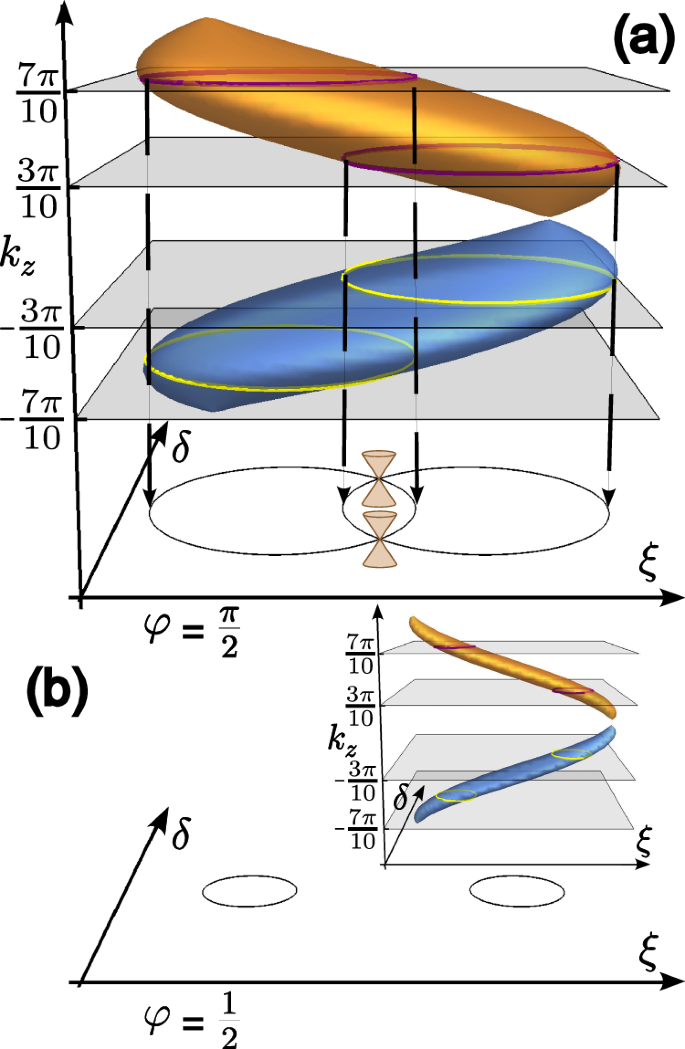
a Top: zero-energy contour (Bogoliubov Fermi surface) of a bulk superconductor under φ = π/2 in the space of ξ, δ, and kz as defined in Eqs. (4) and (5). Planes show four values of kz allowed by open boundary conditions in N = 9 layer flake. Bottom: Projection of zero-energy contours for kz marked in the top panel. 2-D Dirac points form at the points of their intersection. b For smaller value of φ, the contours with the same kz no longer intersect, and no Dirac points are formed.
We note that the above analysis does not include the effects of Htwist(φ), implying that the generation of additional Dirac nodes is a property of a single N-layer nodal superconductor flake. In the N → ∞ limit, however, a Bogoliubov Fermi surface (Fig. 3) should be recovered for a nodal superconductor under current38,39,40. This is consistent with the number of Dirac cones growing as ∝ N2, as the proliferating nodes should cover the area of this surface. In the Supplementary Note 3 we also demonstrate that this generation occurs when a full tight-binding model of N layers is considered, instead of the continuum Dirac approximation.
Current-driven topological transitions
We can now demonstrate that each zero-energy point in ξ, δ space corresponds to a gapped Dirac point with the same Chern number in presence of twist. Using an orthonormal pair of zero-energy eigenstates at a given momentum one can obtain an effective low-energy Hamiltonian by projecting Htwist, Eq. (8) onto the Hilbert space spanned by those two states. The result takes the form
where ki are the vector components of (({k}_{parallel },{k}_{perp },{k}_{z}^{i})), σj is the zero energy basis, (m(varphi ,{k}_{delta }^{j},{k}_{z}^{i})) is the Dirac mass which depends on tz, and ({mathcal{A}}) is a 3 × 3 matrix defined in Supplementary Note 2 which generalizes the mixing of ξ, δ between basis components σ1, σ3. The twist- and current- induced Dirac mass term takes the form
The corresponding Chern number for each node is then ({mathcal{C}}=-frac{{rm{sign}}(m(varphi ,{k}_{delta }^{j},{k}_{z}^{i}))}{2}) due to change in the sign of one of the velocity components (see Supplementary Note 2). However, since (m(varphi ,{k}_{delta }^{j},{k}_{z}^{i}), < ,0), Eq. (29), the Chern number is the same as for the δ = 0 nodes at low current, (20). Thus, we arrive at the conclusion that for finite φ one can generate new Dirac nodes with the same chirality. We remark that for large twist angle case (see Supplementary Note 2), the gap does not appear in lowest order in tz/δ0, suggesting that that regime is unfavorable for the observation of topological transitions.
To illustrate the behavior of the Dirac nodes, we present the sequence of evolutions of the number and chirality of the Dirac nodes as we increase φ from zero. For a specific example, we illustrate the sequence for N = 11 layers in Fig. 4. Once φ > 0, all Dirac nodes acquire a mass and all have the same chirality. Increasing further, we reach the first condition (varphi =frac{2pi }{N+1}) (i.e. case (i), Eq. (21), is satisfied), where we enter a region for (frac{2pi }{N+1}, <, varphi ,<, frac{2pi }{N-1}) where new Dirac nodes split off for all but the extreme nodes (i.e. those corresponding to (pm {k}_{z}^{1})). From the previous analysis, the original net Chern number determined for (0 ,<, varphi ,<, frac{2pi }{N+1}) follows from the sign of the mass term in Eq. (12), and is preserved even when the nodes along ξi split. To do so, nodes along ξi flip their chirality, while the two nodes at ± kδ have the chirality of the original node. Therefore, the total chirality of the three nodes is the same as the node prior to splitting, so that the Chern number of the system is unchanged.
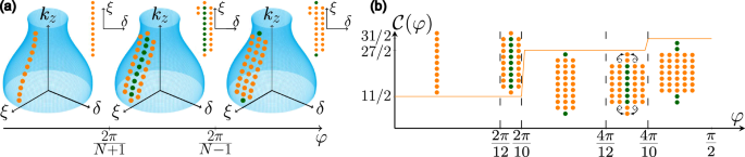
a Evolution of the gapped Dirac node number, position and chirality (marked by color) with increasing φ, related to interlayer supercurrent (cf. Fig. 2a). Insets show the projection of the nodes in the 2-D space of δ and ξ. b Illustrates the mechanism of current-driven topological transitions in the ξ − δ plane. Increasing the current nodes along ξi split and form pairs of nodes along δ. At (varphi =frac{2pi }{10},frac{4pi }{10}) the δ = 0 nodes change chirality, resulting in topological phase transition which increases the Chern number. The dashed circles denote nodes which merged with a node along k⊥ = 0 shown by the arrows at (varphi =frac{4pi }{12}).
The next condition is when (varphi =frac{2pi }{N-1}) (case (ii), Eq. (22), is satisfied). For this case, a gap closing occurs which results in a topological phase transition. Increasing φ further such that (frac{2pi }{N-1} ,<, varphi ,<, frac{4pi }{N+1}), all ξi nodes for k⊥ = 0 reverse chirality due to the gap closing at (varphi =frac{2pi }{N-1}), but not the nodes at δ ≠ 0 formed from splitting discussed above. As a result, there’s a net change in Chern number before and after the closing of (Delta {{mathcal{C}}}_{net}=N-4). To summarize the discussion so far, we’ve completed a sequence for j = 1 where nodes split while remaining in the same topological phase, and then increase the Chern number for increasing φ (Corresponding to case (i) and case (ii) in Supplementary Note 1A, respectively).
If we continue to increase φ, we enter the second sequence for j = 2 where the cycle repeats. Note, however, that upon entering a new sequence, the δ ≠ 0 nodes with ({k}_{z}=pm {k}_{z}^{i}) for i = j, N + 1 − j vanish by merging with a node along the k⊥ = 0 axis as illustrated in Fig. 4b for N = 11. Otherwise, continuing to j = 2, for (frac{4pi }{N+1} ,<, varphi ,<, frac{4pi }{N-1}), a new pair of node splitting occurs at (varphi =frac{4pi }{N+1}) (i.e. all nodes of ({k}_{z}^{i}) split except the four at ({k}_{z}^{i}=pm frac{pi }{N+1},pm frac{2pi }{N+1})) with the same effects on their chirality. Once we increase φ to the next topological phase transition, as before, the Chern number changes but by (Delta {{mathcal{C}}}_{net}=N-8).
Overall, completing each sequence results in topological transitions which compound to increase the Chern number. We can represent the Chern number as a function of φ as:
where ⌊… ⌋ is the floor function used to count the number of transitions that occurred for a given value of φ (i.e. the index j for which ({varphi }^{j}=frac{2jpi }{N-1}) and (lfloor frac{N-1}{2pi }varphi rfloor =j)). For example, taking φ = π/2 and N ≫ 1 we get ({mathcal{C}}(varphi )approx frac{3}{32}{N}^{2}). Therefore, with respect to the number of layers, the Chern number scales as ({mathcal{O}}({N}^{2})).
In addition, we confirmed the sequence of topological transition within a tight-binding model, modeling the effect of twist by an added idxy pairing component, see Supplementary Note 3. This confirms the intuition that twisting the top layer creates an idxy component that “proximitizes” the whole stack while supercurrent in the flake is responsible for the generation of new Dirac nodes.
Comparison with microscopic moiré model
We now compare the numerical solution of the tight-binding model (Sec. II A) with the continuum model. Due to the twist angle being rather close to 45∘, it is appropriate to compare to the limit discussed in Sec. II B. We compute the spectrum numerically on a strip of the moiré superlattices with open boundary conditions along one axis. In Fig. 5 (a), we show the resulting eigenmode spectrum for the N = 3 and θ1,3 structure. The chiral edge modes appear inside a bulk gap, consistent with chiral topological superconductivity. Moreover, the number of modes (6 per edge) is exactly as expected in the case of a “proximitized” flake discussed above. Explicitly computing the Chern number from the bulk following the definition in Sec. IV B matches the number of modes/edge exactly and corresponds to a Chern number of 6. In Fig. 5b, we present the dependence of the minimal, maximal and average topological gaps on N. Remarkably, the analytical and numerical results agree well. Note that the analytical model does not take into account the realistic Fermi surface geometry and moiré reconstruction of the bands, while the microscopic model does, indicating a non-trivial robustness of topological superconductivity in twisted flakes.
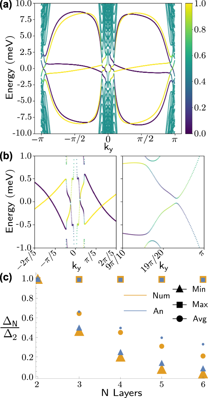
a Quasiparticle dispersion for a 120 unit cell strip of the N = 3 flake with for θ = θ1,3 ≈ 36. 9∘, g0 = 20 meV, and ({varphi }_{c}=frac{pi }{2}) is plotted. The color scale represents the expectation value of position along the open direction. b Displays a closer view of the dispersion of the 6 pairs of edge modes corresponding to a Chern number of 6. Finite size effects induce a small gap in the edge modes near ky = ± π as shown in the right-most figure. c Topological gaps in the microscopic model as a function of N for θ = θ1,2 ≈ 53. 1∘, g0 = 5 meV and high twist continuum model, Sec. II B. The gap values are normalized by the gap size for N = 2. The maximal gap is almost N-independent, reflecting that the twisted layer is largely decoupled from the remaining stack at large twist.
Experimental predictions
We now consider the implications of the topological superconductivity in flakes for two types of experiments: scanning tunneling microscopy (STM) and thermal Hall effect (THE)17. STM gives access to the local density of states of the top layer as a function of position and energy. We will refer to the density of states within a given layer as the projected density of states (PDOS) and the spatially resolved PDOS as the local density of states (LDOS). Choosing energies within the topological gap, the contribution of edge states can be separated. The presence of a topological phase can then be identified by a zero LDOS in the bulk of the system with nonzero LDOS localized at the boundaries. As the topological gap of the top layer can be almost N-independent (Fig. 5c), this opens the path to detecting topological superconductivity in thin/thick flake structures.
We now analyze the LDOS of the top layer. In Fig. 6a we present the LDOS in the 3 layered system of the microscopic model (Sec. II A). A noticeable LDOS is observed only near the system boundary while the interior of the system appears empty for energies below a threshold. For additional clarification, we also show the LDOS for a fixed position as the energy bias varies. Here, the center of the system has zero LDOS until the bias is larger than the gap size, where bulk bands start to contribute. On the other hand, the edges show considerable LDOS at zero bias that actually diminishes on increasing the bias.
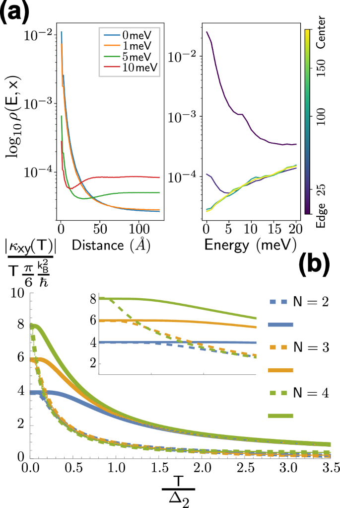
a Local density of states of the top layer of a N = 3 layer system with angle θ1,3, g0 = 20 meV, and ({varphi }_{c}=frac{pi }{2}) along a 120 unit cell strip. The left panel plots the LDOS averaged within each moiré unit cell versus the position of each unit cell’s center along the open axis at fixed energies. The right panel displays the LDOS versus energy for fixed positions between the left and center of the system. LDOS shows a pronounced increase in the bulk above a threshold energy, while below it, LDOS is concentrated at the edges indicating the presence of a topological gap. b Normalized thermal Hall coefficient as a function of temperature normalized by the N = 2 topological gap computed from the microscopic model represented by dashed lines and continuum model (Eq. (12)) in solid lines. The conductance was computed at a cutoff of ∣Ecutoff∣ = 5 meV and g0 = 10 meV.
We note that the LDOS is only strictly zero below the minimal topological gap of the entire flake. To illustrate this point, we compute the PDOS, as outlined in Sec. II A, on the top layer of the Hamiltonian in the large twist limit outlined in Sec. II B using the eigenstates corrected to first order. The PDOS, ρ0(E), for the top layer is given as
which remains gapped even in the N → ∞ limit. However, the N layer stack also provides a contribution of
which becomes gapless for large N. However, for large twist angles tz ≪ δ0, this contribution is suppressed, resulting in a clear signature at the top layer’s gap energy, as confirmed by our numerical results (Fig. 6a).
We now consider the thermal Hall (TH) conductivity κxy(T), that is directly related to the Chern number ({mathcal{C}}) of the system at low temperatures via ({kappa }_{xy}(T)approx -frac{pi }{6}CTfrac{{k}_{B}^{2}}{hslash })17,45,46. At finite temperatures, THE can appear even in non-topological twisted superconductors47, however, the magnitude of the effect is smaller than for the topological ones. Most importantly, it can be used to detect the topological phase transitions, predicted in Sec. II C. To compute κxy(T) we follow the approach of17,48 (see Sec. IV C for details). In Fig. 6b, we present κxy(T) normalized by (frac{pi }{6}Tfrac{{k}_{B}^{2}}{hslash }) computed for the microscopic model of θ1,2 structure and for the low-angle continuum model (Sec. II B) for up to N = 4.
For the continuum model, we first consider the case of current between two top layers only, Sec. II B and Eq. (12) (see also Supplementary Note 2. At low temperatures, all curves reach a plateau with value equal to the Chern number and width related to the energy gap of the system. Comparing results from both models in Fig. 6b, they plateau to the same values, but the reduced energy gap in the microscopic model diminishes the width of the plateau relative to the continuum. Interestingly, away from low temperature, κxy(T) appears independent of the number of layers. This result also follows from the continuum model with the Dirac gaps given by Eq. (12). In the limit (m({k}_{z}^{i},varphi ),ll ,T), κxy(T) is given by:
where we used (mathop{sum }nolimits_{i = 1}^{N}{sin }^{2}[pi i/(N+1)]=frac{N+1}{2}). Note that this result applies to any value of N, and thus readily applies to N = 2 to N = 4 in Fig. 6b. Qualitatively, it arises because, on the one hand, the average topological gap decreases ∝ 1/N, but at the same time the Chern number grows ∝ N. At temperatures much larger then the gap, ({kappa }_{xy}propto {{mathcal{C}}}_{net}langle Delta rangle /T) where 〈Δ〉 is the average gap size, and is thus independent of layer number. This opens the possibility of using finite-thickness flakes to study the appearance of topological SC at the twisted interface.
We now demonstrate that the current-driven topological transitions (Sec. II C) can be studied with the THE. Each transition will correspond to an abrupt increase in Chern number, reflecting in a larger κxy(T) value at low temperatures. To evaluate the TH coefficient, we use the continuum model, Sec. II C and use the Dirac approximation for low energies. In particular, we use the gaps in the Dirac approximation for nodes along δ = 0 from Eq. (20) and for δ ≠ 0 from Eq. (29) applied to the TH coefficient defined in Sec. IV C. We can then sum together the TH coefficient from each node which determines κxy,tot(T).
Figure 7 shows the effect of increasing current through the flake on κxy,tot(T) at low temperature (and therefore the Chern number) in the case of low twist angle (δ0 ≪ tz) and for N = 11 layers in the lowest sequence (i.e. j = 1 for the quantized values of phase in the cases listed in Supplementary Note 1A). When (varphi < frac{2pi }{N+1}), we have a topological gap and a Chern number of (frac{11}{2}) (for a single layer, the total Chern number for all valleys is 2 for a d-wave superconductor), consistent with the contribution of a single gapped Dirac node for 11 layers. Once φ first passes (frac{2pi }{N+1}), the Dirac nodes for all ({k}_{z}^{i}) except for ({k}_{z}^{pm 1}ne pm frac{pi }{N+1}) split, producing a pair of nodes. However, as shown in Sec. II D, the gap does not close during this process and the Chern number remains the same. The results for thermal Hall effect (see Fig. 7, orange curve) are in agreement with these predictions. As the phase is then increased past (frac{2pi }{N-1}) (see Fig. 7, green curve), the value of the plateau suddenly changes. The magnitude of change is (Delta {{mathcal{C}}}_{net}=N-4=7), as predicted in Sec. II D due to the gap closing for Dirac nodes along δ = 0. The plateau range concomitantly increases, reflecting a larger value of the topological gap. The high-temperature behavior appears to converge for (varphi =frac{pi }{12},frac{3pi }{12}) while deviating at (frac{2pi }{11}). The latter value is quite close to the point of topological transition φ = 2π/10, where gap of the δ = 0 Dirac points closes. On the other hand, for (varphi =frac{3pi }{12}) one can check that the gap of the δ ≠ 0 Dirac points is smaller than the δ = 0 ones, such that the high-temperature response is dominated by them, explaining the agreement with (varphi =frac{pi }{12}) result. We note that in this case, the high-temperature limit of κxy(T) would not be independent of N. This is evident for low φ from Eq. (20) which suggests that for a low fixed phase φ ≪ 1/N, κxy(T) would even initially grow proportional to the number of layers. Therefore, even in the non-quantized regime, thermal Hall effect in N + 1 flakes is either as large or larger than in a twisted bilayer. With increasing N such that φ ~ 1/N, this trend is expected to change with the onset of topological transitions.
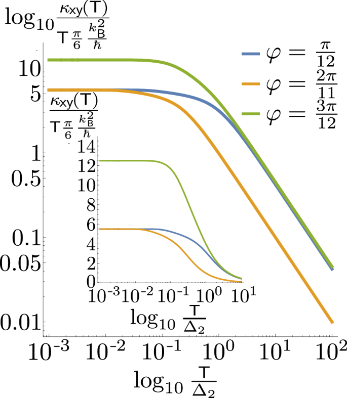
Plotted is κxy(T) normalized by its low temperature limit, κxy(T → 0), versus the temperature normalized by the gap of the N = 2 layered system computed numerically using the continuum model. The abrupt increase in plateau value with φ tracks the current-driven topological phase transition (Sec. II D). The inset displays a closer look at the low temperature limit where THE plateaus to the Chern number, and the onset of (frac{1}{T}) behavior of κxy(T) at intermediate temperatures.
Discussion
In this work we have demonstrated that finite-thickness flakes of nodal superconductors can be used to realize chiral topological superconductivity using current. In Sec. II B we demonstrate in a simplified version of Eq. (6) that the current through the interface between two top layers creates topological superconductivity in the whole flake, “proximitizing” it with an id component formed in the top twisted bilayer17. Analysis of the full continuum model reveals a richer physics with current-induced formation of additional Dirac points (Sec. II C) and topological transition increasing the Chern number up to O(N2) (Sec. II D). Finally, we compare the results of continuum and lattice models in Sec. II E.
We identified that the signatures of the topological phase, such as thermal Hall effect or local density of states reconstruction can be almost independent of the flake thickness (Sec. II F) for a monolayer twisted on top of a thick flake. This platform is an easier alternative to fabricate compared to twisted bilayers, encouraging future experiments. Moreover, the sequence of topological transitions driven by current (Sec. II D) can be detected with thermal Hall effect which we demonstrate in Sec. II F.
The topological states with O(N2) Chern number (Sec. II D) clearly transcend the expectations for N independent layers of 2D topological superconductors and suggests a new phase that can be realized only in finite-thickness flakes. As such, this provides an example of a “2.5″-dimensional effect—one that cannot be observed in either a 3D bulk system (due to vanishing topological gap) or 2D moiré system (where Chern number scales (sim {mathcal{O}}(N))). Instead, in finite thickness flakes the coupling between the layers results in generation of new gapped Dirac nodes and nonlinear scaling of the Chern number with system’s thickness ((sim {mathcal{O}}({N}^{2}))). Combining these observations with effects of magnetic field will pave a way to generate even more elaborate 2.5-D topological superconductors and manipulate their properties17, and promote future prospects of other 2.5-D moiré and heterostructure systems.
Methods
Density of states
The projected density of states (PDOS) in the continuum picture provides contributions which are split between particle- and hole-like components but are restricted to a given layer,
where (k∥, k⊥) compose the coordinate system, (leftvert nrightrangle) indexes the eigenstate and corresponding energy eigenvalue En, and l is the layer index we are performing the projection onto. If performed on a lattice, the integral will be replaced by a sum over a k-mesh in the Brillouin zone normalized by the number of points in the mesh.
The local density of states (LDOS) of the top layer for the lattice model is defined as:
where i enumerate the sites which are positioned at the same coordinate xi in a given layer L. Furthermore, (leftvert nrightrangle) are the energy eigenstates with associated energy En. The eigenstates (leftvert nrightrangle) are expressed in terms of Nambu space with (leftvert {u}_{i}({x}_{i})rightrangle) and (leftvert {v}_{i}({x}_{i})rightrangle) representing the particle-like and hole-like components, respectively, for each site.
Chern number
The Chern number is numerically evaluated by integrating the Berry curvature
In this formula, the Berry curvature is defined in a gauge-invariant fashion as
where (leftvert nrightrangle) and (leftvert mrightrangle) are energy eigenstates with corresponding energy eigenvalues En and Em, respectively.
Thermal Hall
The normalized thermal Hall (TH) conductivity is computed as
where f(ζ) is the Fermi-Dirac function and σH(ζ) is the Hall conductance defined for various energy filling. For the microscopic model, σH(ζ) is expressed as
The normalized TH conductivity can be simplified to the form
which will normalize as T → 0 to the Chern number ∣C∣. Here we compute the TH conductivity within a quadrant of the Brillouin zone (relying on C4 symmetry), resulting in a low temperature value of ∣C∣/4.


Responses