28 nm FDSOI embedded PCM exhibiting near zero drift at 12 K for cryogenic SNNs

Introduction
The ever-increasing computational demand, the advent of artificial intelligence (AI), and the traditional CMOS-based Von Neumann architecture bottleneck have raised a debate concerning computing performance and energy sustainability1,2,3. To circumvent these challenges, it is crucial to explore alternative hardware implementations2,3,4,5. Examples include quantum computers, which operate at cryogenic temperatures and serve as powerful and efficient revolutionary computing platforms. Additionally, energy-efficient brain-inspired systems, including third-generation spiking neural networks (SNNs), are also promising unconventional computing solutions5,6,7,8. Emerging non-volatile memories (eNVMs), such as for instance phase change memories (PCM), stand out as a fundamental building block for scaling and enabling the hardware implementations of these alternative computing solutions9,10. The colocation of memory and processing units in compute-in-memory systems and superconducting processors with cryogenically compatible memory could benefit from reduced latency and energy consumption2,4,7,8.
In the case of cryogenic applications, multiple groups have investigated the behavior and performance of eNVM technologies at cryogenic temperatures, such as ferroelectric11, magnetic12, and oxide-based resistive memories13,14. Results suggest that these CMOS-compatible eNVMs could be used to develop control electronic circuits placed close to the cold core of quantum computers and quantum sensors to avoid thermal noise interference with qubits15. Examples of applications include memristor-based tunable cryogenic DC sources and hybrid circuits for quantum error correction16,17. Additionally, cryogenic-compatible memories combined with brain-inspired computing architectures offer compelling solutions for space exploration due to the scarcity and limitation of resources in systems embedded in satellites18,19,20. Yet, while highly promising, the non-ideality aspects (i.e., variability, retention) and often the lack of eNVMs specifically designed for cryogenic circuits obstruct the progress and development of scalable unconventional computing systems3,21,22.
Among the various types of eNVMs, PCMs are promising and mature solutions for hardware implementations of SNNs in crossbar arrays23,24,25,26. PCMs rely on chalcogenide glasses lying over heating elements. A portion of the active layer undergoes local melting, transitioning between crystalline, amorphous, and polycrystalline phases. It exhibits varying resistance states ranging from low (LRS – crystalline) to high (HRS – amorphous) resistance27. The Ge-rich Ge2Sb2Te5 (GST)-based embedded PCM (ePCM) is proven to exhibit a high level of performance at room and high temperature on high-power automotive and medical applications28,29. However, the ePCM non-ideal resistance drift phenomenon deserves careful attention in the context of multilevel memory systems9,30. The ePCM active layer undergoes structure relaxation over time and the resistance tends to shift towards HRS31,32,33,34. A great deal of effort currently goes into trying to solve this problem through hardware, software, and material-based solutions9,30. While this phenomenon has been extensively reported at 300 K31,32,33,34,35,36,37, there have been limited studies at cryogenic temperatures38,39,40. Most of them are based on GST line cells and are tested on liquid nitrogen as a cooling agent, so the drift is reported at a minimum temperature of 80 K38,39. These studies report the attenuation of drift at cryogenic temperatures but rely on extrapolation to predict an operational range with zero drift38,39. Furthermore, there is a lack of studies exploring the multilevel aspects of GST-based PCMs at temperatures below 100 K40,41. To push the ePCM compatibility even further, with the aim of investigating the potential applications to quantum systems running at minimum temperatures beyond the limits explored so far, 1T1R Ge-rich GST ePCMs fully integrated in 28 nm FD-SOI technology are characterized for the first time at a minimum temperature of 12 K.
The investigation delves deeper into the multilevel programming capabilities and drift aspects of Ge-rich GST-based ePCMs, in SNN applications at cryogenic temperatures. The ePCM is pulse programmed at 300 K, 77 K, and 12 K to achieve and encode 10 resistance state distributions. The threshold location for differentiating neighboring states is set at one standard deviation. To address drift, the resistance evolution was tracked overtime, and the drift coefficient was extracted. A near-zero drift coefficient is observed at 12 K. Finally, to assess and benchmark the effect of drift in SNNs at cryogenic temperatures, a drift modeling is applied to forecast the ePCM multilevel states’ evolution over 2 years. System-level SNN simulations were conducted to evaluate the inference performance in the MNIST classification task. The classification accuracy is sustained at 77 K and 12 K for up to 2 years, while the accuracy drops 10.8% at 300 K. These findings pave the way for the application of ePCM in cryogenic-based brain-inspired computing systems.
Results
ePCM pulse programming
The embedded PCM technology considered in the study is a chalcogenide ternary alloy Ge-rich Ge2Sb2Te5 cointegrated with advanced CMOS technology based on a 28 nm Fully Depleted Silicon On Insulator (FD-SOI) substrate manufactured by STMicroelectronics42. The active layer lies over a wall-type heater element42. A cross-sectional schematic representation of the ePCM is illustrated in Fig. 1. The ePCM cell area is 0.036 µm2/bit. The characterization and pulse programming algorithm of the ePCM cells for analog and multilevel switching were performed at 300 K, 77 K, and 12 K using a test setup that comprised a Keysight B1500A semiconductor analyser with a 200 Msample/s waveform generator module (WGFMU) and a Lakeshore CRX-VF cryogenic probe station (see Fig. 1). Endurance, device-to-device variability, and retention of the ePCM demonstrator considered in the analysis are reported elsewhere42,43,44. Due to sample size restrictions of the cryogenic test setup, only a reticule of the ePCM wafer demonstrator was tested containing three 1T1R ePCM cells.

a 1T1R FD-SOI ePCM stack cross-sectional representation. The ePCM cell area is 0.036 µm2/bit. b The test chip is probed by a CRX-VF cryogenic probe station under continuous refrigeration using helium. The ePCM is connected by a three thermally anchored micro-manipulated probe arm and pulse programmed by a Keysight B1500 semiconductor analyser with a waveform generator module (WGFMU) at 77 K and 12 K.
The voltage-based pulse programming algorithm performed to achieve multilevel states uses constant amplitude SET and increasing amplitude RESET pulses, as depicted in Fig. 2a. SET and RESET sequences exhibit the same symmetric pulse shape of 75 ns for rise, width, and fall times. A complete iterative cycle to span the entire ePCM resistance window incorporates 10 SET and 10 RESET VBL pulses applied to the top electrode of the ePCM cell (bit-line/BL), while a constant DC bias VWL is applied to the gate of the FD-SOI selector (word-line/WL). As shown in Fig. 2b, the 10 SET pulses are constant (1.5 V) while the subsequent 10 RESET pulses are incrementally increased by 0.1 V each step from 1.8 to 2.7 V. VWL ranging from 0.8 to 1.3 V were used to explore different aspects of resistance evolution dynamics. Each VBL programming pulse is followed by a 0.1 V 1 ms VBL reading pulse.
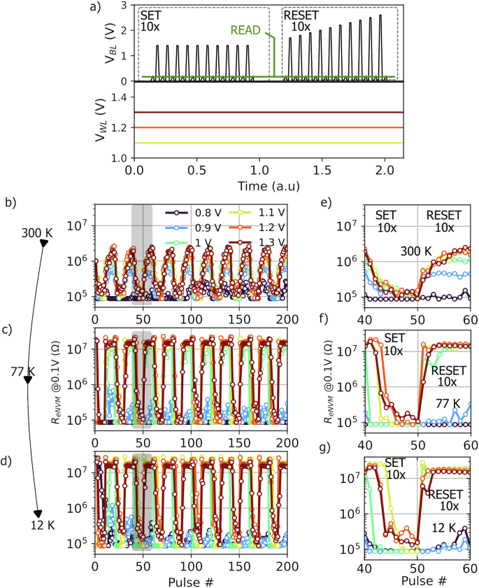
a The voltage-based pulse programming scheme employed to progressively span the entire ePCM resistance window, transitioning from LRS to HRS. b The corresponding resistance evolution (read at 0.1 V) over a sequence consisting of 10 SET pulses of 1.5 V and 10 RESET pulses starting at 1.8 V and ending at 2.7 V. This sequence is repeated 10 times for a total of 200 pulses for each VWL bias from 0.8 V to 1.3 V at 300 K, (c) 77 K, and (d) 12 K. The magnified view of the ePCM response to one SET and RESET sequence is shown for (e) 300 K, (f) 77 K, and (g) 12 K.
As shown in Fig. 2b, the resistance changes progressively in response to the programming pulses at 300 K. On the other hand, at 77 K and 12 K, the resistance evolution is more abrupt. One can see that while the maximum HRS is 3 MΩ at 300 K, it increases to 20 MΩ at 77 K and 22 MΩ at 12 K. Mostly intermediate states and HRS increase when temperature decreases while LRS barely changes and remains within the range of 80–100 kΩ for all temperatures.
This behavior can be attributed to the fact that, according to previous studies, the hexagonal crystalline phase of the GST PCM in LRS exhibits a metallic temperature dependence of resistivity, while amorphous and cubic phases present a semiconductor-type temperature dependence in intermediate and HRS45. Thus, at cryogenic temperatures, the negative temperature coefficient of resistance of semiconductors plays a significant role as the HRS shifts by one order of magnitude from 300 K to 12 K. This different response to temperature for the hexagonal, amorphous, and cubic phases that make up the active region of the PCM from LRS to HRS justifies this abrupt change.
Interestingly, a more resistive eNVM at cryogenic temperature might increase the scalability of an SNN hardware46. In addition, the resistance shift might ease the design requirements of the ePCM selector to achieve the same ON/OFF ratio as at 300 K since the initial pulses of the incremental amplitude RESET ramp are adequate to attain a resistance comparable to the high-resistance state at 300 K.
Inherent multilevel characteristics of ePCMs at different temperatures
To explore and benchmark the intrinsic multilevel capabilities of ePCMs at different temperatures as shown in Fig. 2, sets of programming instructions and encoding schemes are considered to create a list of ePCM states. Note that, from now on, “state” refers to the average resistance achieved for each programming pulse of the programming sequence repeated 10 times. As previously described, the full sequence consists of 20 programming pulses, 10 SET + 10 RESETS programming pulses, and it is iteratively repeated 10 times so that each programming pulse represents a distribution corresponding to a state. Note that the full sequence is applied for five different VWL biasings ranging from 0.8 to 1.3 V, thus the total number of states distributions is 120 (see the average resistance states for each programming pulse depicted in Fig. 3a–c). This first list considers every state distribution. On the other hand, to encode multiple bits with just some of the state’ distribution and programming instructions, a second list of selected states is created, taking into consideration a threshold location or tolerance for a multilevel memory of one standard deviation. To create this second list, a script is used to arrange every state distribution in ascending order from LRS up to HRS and select the maximum number of states that meet the selection criteria of one standard deviation (({rm{sigma }})) as a threshold:
Where ({{rm{mu }}}_{{rm{i}}}) represents the average and ({{rm{sigma }}}_{{rm{i}}}) the standard deviation of the resistance distribution at the ith position in a list, where i ranges from 1 to n, with n being the total number of states in the list. It is thus referred to as a list of “pre-selected” and “selected” states. Both lists are look-up tables comprehending the set of programming sequences/instructions to achieve a corresponding desired resistance state distribution covered so far. The list of pre-selected states contains the entire set of programming instructions and states, while the list of selected ones contains a reduced number of programming instructions and states. Figure 3d–f presents every state distribution of the list of selected states that contains 10 states at 300 K, 77 K, and 12 K.
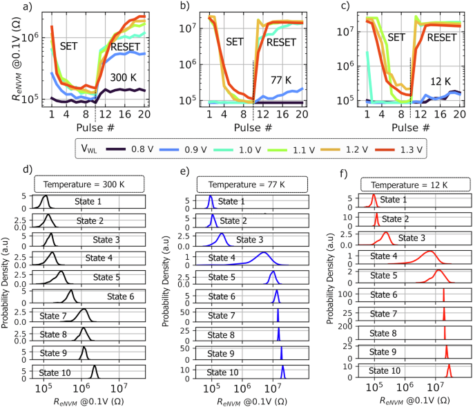
a Average resistance state as a function of the programming pulse iteratively repeated 10 times along the complete programming sequence comprising 10 SET and 10 RESET pulses at different VWL biasing conditions ranging from 0.8 V to 1.3 V at 300 K, (b) 77 K, and (c) 12 K. Each average resistance value is an element of the list of pre-selected states (states before selection) consisting of a total of 120 states and programming sequences. d The list of selected states containing 10 distributions of states extracted from the pre-selected list considering a threshold location for a multilevel memory of one standard deviation at 300 K, (e) 77 K, and f) 12 K.
As shown in Fig. 4, the ePCMs exhibit a broader range of resistance, with an HRS one order of magnitude greater at cryogenic temperatures but the same number of selected states. Note that the selected states are inherent to the pulse programming strategy depicted in Fig. 2. This approach leverages the intrinsic properties of ePCMs through the use of lookup tables and the measured data of the ePCM cells. Previous studies have reported 16 to 32 states at room temperature using the write and verify iterative programming mechanism to control the state distribution and variability9,47. Some neuromorphic hardware-software implementations have also encoded and calibrated the eNVM states based on their intrinsic variability through hardware-aware training8,48,49,50.
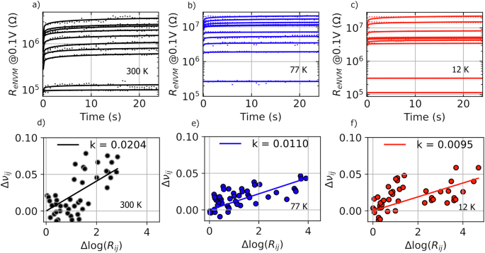
Retention measurements spanning the most prominent drift behavior effectively captured at the first minute after pulse programming at (a) 300 K, (b) 77 K, and (c) 12 K. Reading pulses start at 0.9 ms and are taken at intervals of 0.5 ms. The drift coefficient is obtained by Eq. (2), and the correlation between the drift coefficient and resistance is established by Eq. (3) at (d) 300 K (e) 77 K and (f) 12 K. This leads to pairs of points taken two at a time to compute νRj − νRi and log(Rj/Ri), which are then used to calculate the k coefficient.
Calculation of the drift coefficient at temperatures as low as 12 K
In PCMs, after programming, the active layer undergoes structural relaxation overtime. It leads to resistance drift, overlap, and misreading whenever one considers a PCM multilevel cell. In order to investigate and capture this phenomenon, a drift test at 300 K, 77 K, and 12 K was conducted. The same programming scheme depicted in Fig. 2a is used to first program the ePCM. It is subsequently read at 0.1 V, starting at 0.9 ms after programming, over 30 s, with a reading interval of 500 ms (see Fig. 4a–c). The resistance evolution of five states from LRS to HRS are tracked. The drift phenomenon is then modeled and extracted according to the power law51,52:
Where Rt0 stands for initial resistance at time t0, and Rt instant resistance at time t. Finally, v is the drift coefficient. As the most prominent drift behavior is effectively captured within a confined initial time range34,37,53, the fitting window considered in the analysis is the first minute after amorphization with a view to accurately capturing the distinct shift in resistance within the sub-second range immediately after programming (see Fig. 4a–c). The drift coefficient for LRS and HRS goes from 0.011 to 0.086 at 300 K, 0.00047 to 0.043 at 77 K, and 0.00045 to 0.041 at 12 K. The median and standard deviation of the drift coefficient spanning the entire resistance range are 0.078 ± 0.025 at 300 K, 0.025 ± 0.014 at 77 K, and 0.017 ± 0.018 at 12 K, respectively. A slight change from 0.043 to 0.041 in the maximum drift coefficient is observed at 12 K compared to 77 K. It is noteworthy that the range of the drift coefficient at room temperature is in complete agreement with the literature33,34,36,37,53,54,55, even though it may vary according to the phase change material. As previously mentioned, the ePCM considered in this study is Ge-rich. To date, there have been limited studies at cryogenic temperatures, and most are GST line cell devices. Studies at 80 K and 125 K reported an average drift coefficient of 0.01 and 0.07 at HRS, respectively, and a zero-drift coefficient at approximately 60 K for a line cell based on extrapolations38,39. According to Khan39, the reduction in the drift coefficient at cryogenic temperature is caused by a combination of structure relaxation and diminished kinetic energy and rate of charge emission from electron traps in the amorphous phase. The results shown in Fig. 4 report the drift temperature dependence at 12 K for the first time.
ePCM state distribution evolution over time
Considering the distribution and variability of states, it is essential to model the correlation between the drift coefficient and resistance to forecast the evolution overtime of any resistance state achieved during programming. Since drift is resistance dependent, there is a generalized way of predicting drift using the following equation35,56:
Where νRj and νRi refer to the drift coefficient of a corresponding pair of initial resistances Rj and Ri, respectively measured. k denotes how the drift coefficient depends on resistance. As shown in Fig. 4d–f, the k coefficient is 0.0204, 0.0110, and 0.0095 at 300 K, 77 K, and 12 K, respectively. The k coefficient is also temperature dependent and, as observed, it drops with the temperature.
Once it has been obtained, it becomes feasible to predict the drift coefficient for any resistance state by combining Eqs. 2 and 3, as follows:
Consequently, when applied to the list of states depicted in Fig. 3, it becomes feasible to predict and project the resistance distribution evolution at any given moment (see Fig. 5). The study comprises a huge exploration range from seconds to approximately 2 years.
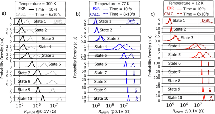
The distribution of the 10 experimentally extracted and encoded selected states at (a) 300 K, (b) 77 K, and (c) 12 K read at time 10−3 s (≈0.9 × 10⁻³) and their projected version after approximately 2 years of drift (6 × 10⁷ s), calculated by Eq. 4.
The impact of ePCM drift on SNN performance at temperatures as low as 12 K
Once the projection of states’ distributions over time had been obtained for each temperature, a system-level simulation was carried out on a fully connected SNN to evaluate and compare the effect of state overlap and misreading caused by drift on ePCMs. Both lists of states (pre-selected and selected) are used and considered separately to assess whether a reduced number of states and programming instructions is enough to achieve reasonable accuracy. In system-level simulations, the weight matrix, or synaptic strengths in SNNs, are counted as conductance states. Weight normalization is a common practice used to improve stability, convergence, and performance in simulations. Therefore, the list of states pre-selected and selected at 300 K, 77 K, and 12 K is thus converted to conductance C and to a normalized weight state ranging from 0 to 1,
where Gmin is the minimum conductance, Gmax is the maximum conductance, and G is the conductance of the device. It covers both the experimentally extracted resistance state distributions and those predicted using Eq. (4). The normalized conductance states are used to simulate an ePCM-based SNN for the MNIST classification task. A feedforward 784×50 spiking neural network is considered as depicted in Fig. 6a. A fully connected network is the basic building block in deep networks and the readout layer of more sophisticated topologies like convolutional (CNNs) and recurrent neural networks (RNNs). the objective is to characterize the impact of drift on a simple network to clearly evaluate the fundamental impact of drift, temperature, and quantization on network weights. The computation process involves a 28×28 grayscale image rate encoded into spike trains using 784 input LIF neurons. When a pre-synaptic neuron fires, it sends a spike through the ePCM synapse, which modulates the spike based on its stored weight. The weighted signals are summed at the 50 post-synaptic neurons in the crossbar array, representing the last layer of the SNN. Larger networks allow learning receptive fields areas or distinct features for each class57,58, meaning that each class is represented by more than one neuron. The post-synaptic neuron integrates the currents and fires if a threshold is exceeded. The training method is based on the unsupervised learning rule called “voltage dependent synaptic plasticity” (VDSP)58,59. The SNN is trained, and the corresponding software-based computed weights are compared to the experimentally extracted lists of pre-selected and selected ePCM states to find the nearest corresponding value. The trained weights are updated, or replaced by the nearest corresponding normalized states, and sorted by their standard deviation to define the final weights used to compute inference on a test set before drift. On the other hand, to evaluate the effect of drift on classification accuracy at different times, the final weights used to compute inference before drift are replaced by their projected counterpart obtained through Eq. (4), as depicted in Fig. 5. The calculation begins at 6 s and progresses logarithmically up to approximately 2 years, reaching 6×10⁷ s. Henceforth, the inference is computed without further training steps, ensuring that the trend in the evolution over time of the classification accuracy remains consistent regardless of the training method considered in the analysis, enabling the generalization of the study. The baseline accuracy before updating the weights by the list of states is 72.5%. After weight update with the ePCM pre-selected and selected list of states, the latter achieves an average classification precision of 71.7%, 69.5%, and 70.9% while the former reaches 71.5%, 69.6%, and 70.7% at 300 K, 77 K, and 12 K, respectively (see Fig. 6b–c). The MNIST classification performance is in complete agreement with the literature for similar PCM based SNN architectures60,61. Considering the standard deviation, the performance is barely distinguishable between temperatures and encoding schemes (selected and pre-selected list) prior to the occurrence of the drift phenomenon – Possibly because both lists span the entire resistance range regardless of the number of states and present a similar average coefficient of variability (CV) per state in the order of 15%, initially.
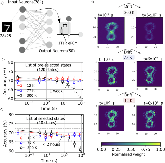
a SNN implementation of an MNIST classification task composed of 784 (28 × 28) rate-encoded input LIF neurons and 50 output neurons, meaning that each class is represented by more than one neuron, with synaptic weights represented by 1T1R ePCMs. b The inference classification accuracy out of 10 seeds at 300 K, 77 K, and 12 K considering both ePCM multilevel encoding approaches, pre-selected (120 states), and (c) selected list of states (10 states) at different times to account for resistance drift. The baseline accuracy is 72.5% and the average accuracy prior to drift is 71.7%, 69.5%, and 70.9% for the pre-selected list of states and 71.5%, 69.6%, and 70.7% for the selected list at 300 K, 77 K, and 12 K, respectively. After 2 years of drift the former reaches 60.9%, 69.5%, and 70.1% and the latter 60.6%, 68.1%, and 69.3% at 300 K, 77 K, and 12 K, respectively. d The weight matrix (receptive fields) for an output neuron over time t = 10−3s and 2 years (t = 6 × 10⁷s).
Now, considering the predicted version of the selected and pre-selected list of states starting at 6 s going towards 6 × 10⁷ s, the pre-selected list of states achieves after 2 years (6 × 10⁷s) a classification performance of 60.9%, 69.5%, and 70.1% while the selected list of states reaches 60.6%, 68.1%, and 69.3% at 300 K, 77 K, and 12 K, respectively (see Fig. 6b, c). The impact of the more pronounced drift at room temperature compared to cryogenic temperatures is evident: the latter undergoes a performance drop of 10.8% while the former presents a sustained precision along the complete time window irrespective of the list of states under consideration (see the receptive fields in Fig. 6d). The accuracy consistently declined over time at room temperature in both scenarios, starting to drop 1 week and two hours after programming for the list of pre-selected (120) and selected (10) states, respectively. This difference in time possibly arises due to a larger number of states being available on the pre-selected list that are more prone to being closer to the original trained weights from simulation. The likelihood of the states being closer to the original distribution simply means that they are more likely to be closer to the center and distant from the edges of the distribution of the original trained states, and consequently farther from the threshold for state overlap and misreading. This suggests that it would require more time to drift and overcome the threshold barrier for misreading compared to the list of selected states.
As both encoding schemes present a similar accuracy at 77 K and 12 K the entire time, this means that the less costly approach comprising the list of 10 defined states and programming instructions is preferable compared to the list of 120 pre-selected states. However, at 300 K the latter must be considered to sustain the accuracy over 1 week instead of two hours.
It is essential to emphasize that baseline accuracy is proportional to the number of output neurons58,59. For instance, a state-of-the-art accuracy of 90% could be achieved in a VDSP-based SNN comprising 500 output neurons58,59. However, using 50 output neurons is sufficient to adequately depict the effect of drift and temperature on classification accuracy over time, while simultaneously minimizing computational expenses.
In sum, it should be noted that ePCM performance at cryogenic temperatures in SNN applications is enhanced due to this inherent drift mitigation aspects. The accuracy is sustained over 2 years and a less costly encoding approach is favored at cryogenic temperatures. It thus enables and attests to its efficient application in spiking neural networks at cryogenic temperatures down to 12 K due to this near-zero drift condition without requiring any additional software or hardware solution to address drift mitigation.
Discussion
The study presents the performance enhancement of multilevel 28 nm FD-SOI embedded phase change memories at cryogenic temperatures. It is shown, for the first time, that the intrinsic non-ideality aspects of resistance drift in Ge-rich GST ePCMs are suppressed at 77 K and 12 K while maintaining the same programming requirements as at 300 K. The voltage pulse programming strategy is employed to explore the multilevel capability aspects of the ePCM at room temperature and cryogenic temperatures. Different encoding schemes are considered to assess whether a reduced number of states and programming instructions is enough to achieve a reasonable accuracy in an SNN classification task. Ten multilevel resistance states (list of selected resistance states) are encoded out of 120 programming instructions (list of pre-selected resistance states) considering a threshold location for a multilevel memory of one standard deviation at 300 K, 77 K, and 12 K. The drift aspects are characterized and modeled to estimate and forecast the change in the multilevel resistance states over time. A near-zero drift coefficient is observed at cryogenic temperatures. The comprehensive system-level simulation conducted on a fully connected SNN for the MNIST classification task verifies the efficacy of drift mitigation at cryogenic temperatures. The average inference accuracy drops by 10.8% at 300 K while it is sustained at 77 K and 12 K over 2 years regardless of the encoding approach, whether containing 10 or 120 states. However, the results suggest that the encoding scheme plays a role at 300 K; the accuracy of the selected states approach declines sooner, occurring two hours after programming, in contrast to a week when considering the 120 pre-selected states. This shows that at cryogenic temperatures, SNN-based ePCMs not only preserve accuracy for as long as 2 years but also facilitate the use of a simpler encoding method without compromising classification performance. These findings indicate that ePCM emerge as a highly promising cryogenic-compatible memory solution – and more importantly, without requiring any additional hardware or software solution for drift mitigation. In light of this, the employment of an ePCM is quite appealing for applications in unconventional brain-inspired computing systems, such as SNNs, cryogenic memories for quantum systems, and embedded aerospace circuits.
Methods
Electrical characterization
The electrical characterization was performed on a Keysight B1500A semiconductor analyser with a 200 Msample/s waveform generator module (WGFMU) and a Lakeshore CRX-VF probe station under continuous refrigeration using helium. The WGFMU modules and source measure units (SMUs) are controlled using an external computer via the GPIB interface. A code in C language encompasses the GPIB commands for the pulse programming routine.

Responses