Bayesian stability and force modeling for uncertain machining processes

Introduction
Milling is a common machining process used to produce high-precision components1. Producing parts for maximized profit requires selecting milling parameters, such as depth of cut and spindle speed, that minimize cost. However, there are physical constraints on this optimal parameter selection. Some sets of cutting parameters may cause chatter which damages the part and tool2,3. Others may be stable, but not provide the required part geometric accuracy or surface finish4,5. Others could exceed the machine tool’s capabilities, such as the maximum spindle power output6. Therefore, selecting optimal milling parameters requires the ability to predict whether a cut will be stable and produce acceptable parts under realizable conditions. To enable pre-process selection of milling parameters, milling simulation has been widely studied in the literature. For example, chatter can be predicted by calculating a stability map based on the cutting force model and system dynamics7,8,9, while surface location error predictions estimate part errors due to the relative vibration of the tool and workpiece10,11. The simulation performance predictions can be used to optimize the milling process by selecting the most productive, realizable parameters.
However, these predictions are subject to both epistemic and aleatoric uncertainty. Epistemic uncertainty is attributed to a lack of information about the system and the model inputs, such as the tool tip frequency response function (FRF) and cutting force model required to calculate the stability map12. Measuring these parameters requires specialized instruments, such as cutting force dynamometers and impact hammers/accelerometers, which are not widely available in the industry. Therefore, in practice, these parameters may not be measured. Furthermore, even if the measurements are performed, there is always uncertainty associated with the measurement results. For example, accelerometer mass loading13 and changes in spindle dynamics with spindle speed14 can introduce uncertainty into FRF measurements. Cutting force measurements are subject to dynamometer dynamics and can vary with milling parameters or as the tool wears15.
While epistemic uncertainty can be reduced by measurements, aleatoric uncertainty is unattributable stochastic uncertainty which must be modeled as essentially random. This is traditionally assumed to be unpredictable variations that may change between tests, such electrical noise in a sensor signal or cutting force variations due to tool wear12. However, it can also be used to describe errors in the machining simulations themselves. Stability algorithms are uncertain due to assumptions or factors not included in the model, which are separate from uncertainty in the model inputs. As an example, the zero-order approximation (ZOA) frequency domain method developed by Altintas and Budak is widely used because of its computational efficiency, but it is less accurate for low radial immersion cuts16. Alternate stability algorithms may be more accurate, but they are generally more computationally expensive2,3,17,18.
Due to these difficulties, data-driven and machine learning methods for identifying the stability map have become a major research focus. These approaches extrapolate the stability map from a small set of cutting tests. For example, Kawai et al. used Gaussian processes19, Greis et al. compared support vector machines, k-nearest neighbors, and neural networks20, Postel et al. proposed both deep neural networks pre-trained by physics models21 and a genetic algorithm approach for inverse parameter identification22, and Deng et al. trained their model using limiting axial depths rather than binary stable/unstable test results to reduce the required number of data points23. However, these methods have some limitations. First, they usually require many cutting tests to learn the stability map and, more critically, may not identify tests for optimal learning. As a result, these approaches are best applied to correct errors in a calculated stability map, rather than as a replacement for system measurements. Second, while these approaches can learn the stability map for one specific case, they are not typically generalizable. For example, while the approaches can predict stability under the same conditions that were used for training, they may not extend to a different work material or radial depth of cut. Third, these methods have focused on stability and have not considered other inputs, including the available spindle power, required surface finish, and dimensional tolerances.
Bayesian modeling is a probabilistic approach to modeling and updating problems. The approach assigns a probabilistic prediction about the system parameters and then updates it based on a series of observations. Authors have applied this approach to model cutting forces24, surface roughness25, and surface location error26,27. Bayesian stability models assign probabilistic predictions about how likely a given set of cutting parameters is to be stable, rather than a binary stable/unstable classification predicted by a stability algorithm. This approach was first proposed by Karandikar et al. with a non-physics-informed Bayesian stability model. They addressed the first issue by allowing the user to select cutting tests which provide new information about the system28. However, they did not connect the final stability predictions to system parameters.
Physics-based Bayesian machining modeling is a more recent area of study that directly connects the stability modeling uncertainty to the uncertainty in the machining system parameters. These approaches establish an initial probabilistic input (called the prior) for the system dynamics and cutting force model and then update those probabilistic inputs based on a series of cutting tests to reduce the system uncertainty. Li et al. proposed the first method in 2020, updating a measured FRF to account for shifts in spindle dynamics at higher spindle speeds29. Cornelius et al. demonstrated that Bayesian stability modeling can be used to select productive machining parameters and showed how assumptions in the ZOA stability algorithm can cause errors in the predicted stability map30. Chen et al. used a surrogate machine learning model to reduce computational time by approximating the output of the stability algorithm31. Schmitz et al. established the prior for the dynamics using receptance coupling substructure analysis (RCSA) and incorporated the measured chatter frequency into the Bayesian updating to learn more from each test cut32. Ahmadi et al. applied Bayesian learning to turning and used the measured tool vibrations to help learn the system dynamics from stable cuts33. Akbari et al. extended the work in ref. 32 by demonstrating a new test selection approach focused on reducing uncertainty in the stability map and showing how the measured parameters can be used to model cutting test results across multiple machine tools34. Cornelius et al. scaled the Bayesian approach to utilize high-performance computing resources and learn process damping35.
Compared with the previous data-driven approaches, physics-guided Bayesian methods address two challenges. First, the current knowledge about the system can be used to select informative test cuts, either to improve productivity30,32 or to reduce stability uncertainty34. This minimizes the number of required cutting tests and the amount of required machine time. Studies have shown that highly productive cutting parameters can be selected in less than 10 cuts32. Second, because these methods learn the underlying system parameters, they can theoretically be used to calculate the stability map for different conditions, e.g., at a different radial width than the original tests or across multiple machines34. However, multiple combinations of system parameters generate similar stability maps, so it may not be possible to uniquely identify the true system based solely on stability results. To date, this has not been fully investigated. The Bayesian models have, so far, focused on stability and have not considered other constraints on machining parameters.
This paper describes a physics-based Bayesian approach for statistically simulating machining operations under a state of uncertainty and establishing probabilistic predictions about the process. It extends prior research by considering other factors about the machining process in addition to stability. These predictions are used to select a series of cutting tests that provide new information about the system and identify increasingly productive machining parameters. Compared with existing Bayesian algorithms, this paper provides three new contributions:
-
1.
demonstrating how Bayesian machining modeling can be extended to include cutting force modeling and spindle power measurements and evaluating how this affects convergence to the true system parameters;
-
2.
proposing a likelihood function based on aleatoric uncertainty that increases explainability and relates it directly to the Bayesian algorithm’s predictive capabilities; and
-
3.
defining a new, computationally efficient test selection method designed to reduce uncertainty in the underlying system parameters.
The paper is organized as follows. “Results” Section describes the proposed Bayesian framework and describes the results of numerical and experimental case studies. “Discussion” Section discusses the results and provides suggestions for future research. “Methods” Section provides detailed information on the case studies necessary for replication. Code for the case studies can be found at the Github repository linked in the Code Availability Statement at the end of this paper. The supplementary information available along with this paper contains additional figures showcasing the uncertainty reduction test selection method.
Results
This section describes the Bayesian milling model and demonstrates it using two case studies. There are five general steps, illustrated in Fig. 1.
-
1.
The user defines a prior distribution describing their initial uncertainties about the frequency response function (FRF) and cutting force model.
-
2.
The prior samples are propagated through a stability map algorithm to create probabilistic predictions about the system and test cuts.
-
3.
The predictions are used to recommend and perform an informative test cut based on the user’s goal, such as improving productivity or reducing system uncertainty. Testing halts if there is no recommendation.
-
4.
A new posterior distribution is defined which incorporates the information gained from the previous test cut using the likelihood function.
-
5.
New samples are drawn from the posterior distribution and returned to propagate through the physics algorithms and create updated predictions.

Flowchart outlining the proposed Bayesian process.
This framework is modular and can be customized depending on the user’s goal and knowledge about the system. For example, new physics algorithms can be added to simulate different aspects of the milling operation, the likelihood function can be customized depending on the type of information gathered from each test cut, and different methods can be employed to sample the posterior distribution. These options are described in more detail in Section “Prior definition” through “Markov Chain Monte Carlo sampling”. Section “Verification studies” shows two verification studies which demonstrate the framework, one numerical and one experimental.
Prior definition
Let (theta) be a variable that defines the machining system and provides enough information to calculate the physics models (described in Section “Physics models and probabilistic simulation”). This variable can take many different forms, but for stability modeling (theta) must at minimum define the cutting force model and FRF. This paper uses the form shown in Eq. 1. The cutting force is modeled using a mechanistic cutting force model, where ({K}_{s}) is the specific cutting force in N/mm2, (beta) is the cutting force angle in degrees describing the ratio between the normal and tangential cutting forces ({F}_{n}) and ({F}_{t}) respectively, and ({k}_{{te}}) is the tangential edge coefficient in N/mm1. Eq. 2 shows how these are used to calculate ({F}_{t}) and ({F}_{n}). This omits the normal edge coefficient ({k}_{{ne}}) since it is not relevant for calculating stability or the spindle power. The FRF is defined as a mass-spring-damper system with natural frequency ({f}_{n}), stiffness (k), and damping ratio (zeta). This can also be extended by including additional modes, as shown in the experimental case study.
These parameters can be converted to different forms for convenient calculation. For example, the modal parameters ({theta }_{{f}_{n}}), ({theta }_{k}), ({theta }_{zeta }) can be converted into the mass-spring-damper values ({theta }_{m}), ({theta }_{k}), ({theta }_{c}) respectively using Eq. 3. The force model parameters ({K}_{s}) and (beta) can be converted into the tangential and normal cutting force coefficients ({k}_{{tc}}), ({k}_{{nc}}) as shown in Eq. 4. These coefficients model the tangential and normal forces shown in Fig. 2. The remainder of this paper uses these conversions to provide the most convenient form for any equation.

Normal and tangential cutting forces acting on the tool
Once the general form for (theta) has been determined, the user defines a prior distribution (Pleft(theta right)) which encodes the epistemic uncertainty for the system, e.g., by defining a mean and standard deviation for each variable. There are many ways to set the prior. Li et al. measured the system dynamics by tap testing29, while Schmitz et al. used receptance coupling substructure analysis32 to predict the tool tip FRF. This paper uses relatively uninformed priors to demonstrate how the Bayesian algorithm can identify the system despite having little initial information.
Once the prior is established, a set of samples can be drawn from that distribution. Each sample ({theta }_{i}) is a given set of parameters that define the system. Since the prior is generally a standard distribution like a multivariate normal or uniform distribution, there are functions available to draw samples from the distribution. Figure 3 shows 4000 samples drawn from the prior distribution for the numerical case study shown in Section 2.6.1. This specific prior is intentionally set to be very broad to help evaluate whether the Bayesian model can converge under worst-case conditions.

The on-diagonal boxes are histograms showing the marginal distribution for each variable, while the off-diagonal boxes show the conditional distribution of the two relevant variables defined by the row and column.
Physics models and probabilistic simulation
Once the prior has been established, it is propagated through a series of physics models via Monte Carlo sampling. Each physics model takes one of the sampled system parameters ({theta }_{i}) and uses it to predict the system or the outcome of a cut, such as the cut stability (stable or chatter) or the cut spindle power. In this study, three physics algorithms are used to estimate the system frequency response function (FRF), cutting stability and chatter frequency, and spindle power.
System frequency response
The complex-valued FRF is calculated first for a given frequency f in Hz using Eq. 5, assuming the system has symmetric dynamics in the (x) and (y) directions (i.e., that ({FR}{F}_{{xx}}={FR}{F}_{{yy}})). For multiple modes, the FRF is calculated for each mode and then summed. Performing this calculation for each sample drawn from the prior gives a probabilistic prediction for the system dynamics. Figure 4 shows the prior distribution of natural frequencies for the numerical case study shown in Section “Numerical study”. In that example, the prior is inaccurate and overestimates the natural frequency. Alternatively, the FRF could be calculated using RCSA34. In this case, the (theta) variable would contain information on the model parameters, such as the connection between the tool and holder, rather than a set of modal parameters.
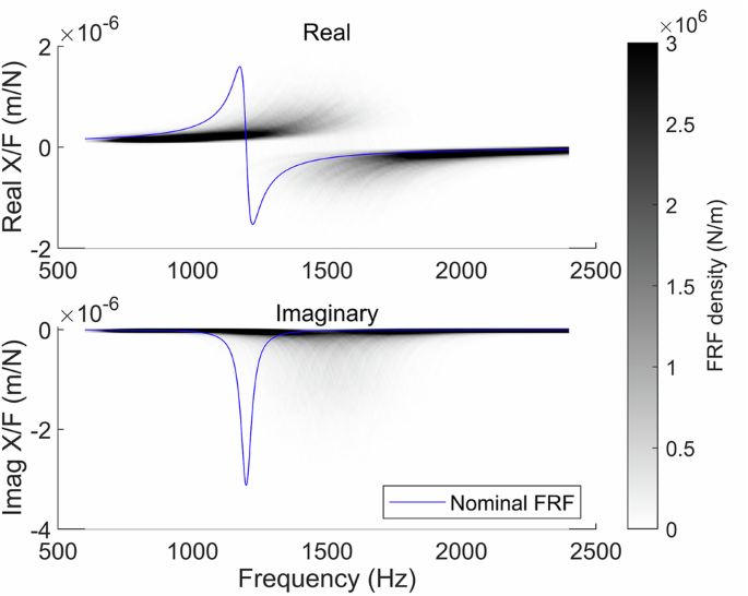
Probabilistic prediction for the X-direction system FRF. Darker regions indicate a higher density of FRF predictions.
Stability prediction
The system parameters are then used to make predictions about the outcome of the milling operation. A straight-line cut can be defined by its radial depth of cut (a), axial depth of cut (b), spindle speed (n), and feed per flute ({f}_{z}). Let (omega) be a vector variable containing all cutting parameters for a given cut. The spindle speed is then ({omega }_{n}), for example. The stability of any given cut (Sleft(theta ,omega right)) can be predicted using a variety of algorithms. This paper employs the well-established ZOA stability algorithm, which removes the time-dependent component of the stability problem by truncating the frequency domain dynamic forces to only the mean component7. See refs. 1,7 for a full derivation of this algorithm. Compared with other stability algorithms, the ZOA is fast to calculate but is less accurate at lower radial depths of cut16. For each spindle speed, radial depth, and set of system parameters (theta), it calculates a limiting axial depth ({b}_{lim}left(theta ,{omega }_{n},{omega }_{a}right)). Cuts at axial depths lower than ({b}_{lim}) are assumed to be stable ((Sleft(theta ,omega right)=1)), while cuts above ({b}_{lim}) are predicted to be unstable/chatter ((Sleft(theta ,omega right)=0)). The most productive cutting parameters offer the highest material removal rate (MRR) without exceeding the stability boundary, as shown in Fig. 5.

Stability map calculated using the ZOA algorithm.
Each sampled FRF is used to calculate a stability map and the combination of all those stability maps defines the probabilistic stability map, where ({P}_{S}left(omega right)) is the probability of stability for a given set of cutting parameters. The probability of stability can be calculated in two ways. The simpler method is to treat the stability predictions as deterministic and calculate what percentage of samples predict a given set of cutting parameters will be stable, as shown in Eq. 6.
However, each stability prediction has aleatoric uncertainty, caused by uncertainty in stability classification and assumptions in the stability algorithm. While the stability algorithm predicts that ({b}_{lim}) is the true stability limit, ({b}_{lim}^{* }) may be either above or below that value, even if the system parameters (theta) were known perfectly. Rather than assigning a binary stable/unstable prediction, the stability algorithm instead assigns a likelihood of stability ({L}_{s}left({S}_{{ex}},omega |theta right)) which states how likely a cut (omega) is to experience a stable or unstable result ({S}_{{ex}}) for a fixed set of system parameters (theta). Let ({sigma }_{b}) be the standard deviation associated with the predicted ({b}_{lim}) value. There is a 68% probability that ({b}_{lim}^{* }) lies within the range ({b}_{lim}pm {sigma }_{b}), a 95% probability that ({b}_{lim}^{* }) is between ({b}_{lim}pm 2{sigma }_{b}), and so on. The likelihood that a given axial depth (b) is above ({b}_{lim}^{* }) (and will chatter) is given by the cumulative density function (CDF) for a normal distribution with mean (mu) and standard deviation (sigma) evaluated at point (x), as shown in Eq. (7). Figure 6a shows how this represents the true stability boundary as an uncertainty centered around the nominal predicted stability limit. Figure 6b compares the proposed aleatoric likelihood to the sigmoid likelihood used by Akbari et al.34. and the Gaussian dropoff used by Karandikar, Schmitz, and Cornelius et al.30,32,35. In practice, these functions behave similarly, but the CDF approach provides a more intuitive definition for the likelihood hyperparameter by associating it directly with the aleatoric uncertainty for the stability prediction and measurement. This function can be customized depending on the specific form of the stability uncertainty, for example, to express ({sigma }_{b}) as a percentage of ({b}_{lim}) rather than as a fixed value.

a Uncertainty boundary for a stability boundary using ({sigma }_{b}=) 0.01 mm. b Comparison between the proposed Gaussian CDF likelihood function and the sigmoid and Gaussian dropoff likelihoods. The Gaussian dropoff and CDF methods use ({sigma }_{b}=) 0.01 mm, while the sigmoid uses (k=) 0.005 mm to match the Gaussian CDF.
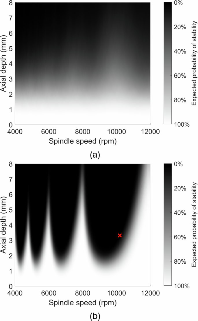
Equation 8 shows how the probability of stability can be calculated using the stability likelihood function. Figure 7 compares probabilistic stability maps generated by these two approaches, showing how incorporating the aleatoric uncertainty decreases the confidence in the stability boundary. To make the difference obvious, the aleatoric uncertainty has been set to ({sigma }_{b}=) 1 mm. This value is so high that the probability of stability at the stability boundary local minima never reaches 100%, even at zero axial depth. In practice, ({sigma }_{b}) should be set based on the user’s expectations about how closely the stability algorithm will predict the true behavior of the machine.

a Stability map with no aleatoric uncertainty. b Stability map with aleatoric uncertainty (({sigma }_{b}=) 1 mm). The color indicates the probability that a cut will be stable. Lighter colors indicate a high probability of stability, while dark colors indicate a high probability of chatter.
The ZOA stability algorithm also provides a chatter frequency estimate for a given cut, ({f}_{c}left(theta ,omega right)). Refer to ref. 32 for more details on how the dominant chatter frequency is extracted for a given sample. Similar to the stability classification, there is aleatoric uncertainty for these chatter frequency predictions. Let ({f}_{c}left(theta ,omega right)) have a standard deviation ({sigma }_{{f}_{c}}). Based on this, the likelihood of encountering a specific chatter frequency ({{f}_{c}}_{{ex}}) is given by Eq. 9, where ({mathscr{N}}left(x,mu ,sigma right)) is the probability density of a normal distribution with mean (mu) and standard deviation (sigma) evaluated at a value (x). In practice, the likelihood should be between 0 and 1, so the non-normalized version shown in Eq. (10) can be used instead. This is equivalent to the Gaussian dropoff approach presented by Schmitz et al.32.
Equation 11 gives the probability of encountering a given chatter frequency considering both aleatoric and epistemic uncertainty. Based on this, Fig. 8 shows a probabilistic prediction for the chatter frequency.

Areas with darker colors have a higher probability of being the true chatter frequency.
Spindle power
The cutting forces on the tool govern the power that the spindle motor must output to perform a given cut. If the motor is not able to output the required power, the spindle will stall. Due to the inertia of the rotating tool assembly, cuts are generally limited by the average cutting power, which can be estimated based on the mechanistic force model1,6. The tangential cutting force applied to a single flute on the tool is given by Eq. (12), where ({k}_{{tc}}) is the tangential cutting force coefficient (see Eq. (3)) and ({k}_{{te}}) is the tangential edge coefficent. The first term models the cutting force as proportional to the chip area. Since the chip area is related to the volume of material removed from the part, the cutting power ({bar{P}}_{c}) associated with this term is given by Eq. (13), where ({N}_{t}) is the number of flutes the tool.
The second term in Eq. (11) models the edge rubbing force and is proportional to the total length of the cutting edge engaged with the part. Since the flute is moving at a surface speed of ({v}_{c}=frac{npi d}{60}), the rubbing power while the flute is engaged with the part is ({V}_{c}cdot {k}_{{te}}b). In milling, each flute is only in contact with the part some fraction of the time ({p}_{{engage}}), given by Eq. (14), where (d) is the diameter of the cutting tool. Equation (15) gives the average rubbing power consumption for all the flutes on the tool. Summing this power with the cutting power for a given set of system parameters (theta) and cutting parameters (omega) gives the total power consumption (bar{P}left(theta ,omega right)), shown in Eq. (16). Note, however, that this equation is only applicable for stable cuts. Unstable cuts can have high amplitude vibration that causes the tool to disengage from the workpiece, altering the force. The spindle power model in Eq. (16) also neglects tool deflection, which can cause the actual engagement of the tool to be slightly larger or smaller than nominal.
To incorporate the aleatoric uncertainty, let ({sigma }_{bar{P}}) be the standard deviation for the spindle power prediction. The likelihood function for experiencing a specific spindle power ({bar{P}}_{{ex}}) is given by the same approach as the chatter frequency prediction, shown in Eq. (17). Alternatively, the power uncertainty can be expressed as a percentage of the predicted value ({sigma }_{bar{P} % }) using Eq. (18). Note that the spindle power likelihood can be omitted when the test cut is unstable since the spindle power estimation is less accurate during chatter. See the numerical case study in Section “Numerical study” as an example.
Propagating the prior samples through Eq. (16) gives a probabilistic estimate for how much spindle power any cut will require (due to uncertainty in ({k}_{{tc}}) and ({k}_{{te}})). Figure 9 gives an example, showing the distribution of possible spindle powers for one set of cutting parameters.

Probabilistic spindle power prediction at 12000 rpm, 8 mm axial depth.
Test selection methods
Once the probabilistic predictions for milling stability and spindle power have been established, they can be used to select a new cutting test based on the user’s goal. Here, two different test selection strategies are described. First, the MRR maximizing approach presented in ref. 32 is used. This approach selects the most productive possible cutting test parameters which conform to the user’s selected risk tolerance for encountering chatter. A risk tolerance of ({R}_{{stable}}=) 0.75, for example, indicates that the user is willing to perform cutting tests only if there is at least a 75% probability of the cut being stable. Based on this risk tolerance, the most productive cutting test is selected using Eq. (19), where (Omega) is the set of all possible cutting parameters for the tool. Figure 10 demonstrates this approach, showing how the test is selected using lines of constant MRR and the risk tolerance boundary.
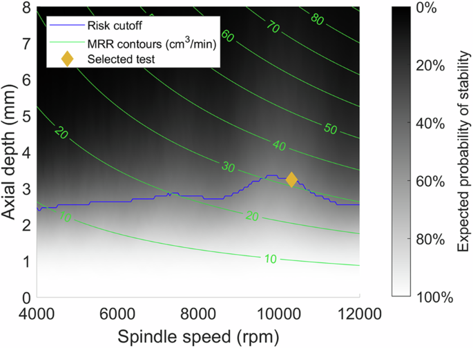
Cutting parameters below the risk cutoff have acceptable risk, while parameters above the cutoff exceed the user’s risk tolerance.
However, this MRR maximizing approach requires a certain level of confidence to select new tests. For highly uncertain systems, there may not be any productive points with a high probability of stability. Instead, tests can be selected to provide new information about the system. The following algorithm selects cutting tests based on the expected reduction in uncertainty for some variable, e.g., the natural frequency for the tool tip FRF. This builds on a method described by Karandikar et al. for reducing process damping uncertainty36 by extending it to other variables, providing a faster method for estimating the posterior uncertainty and incorporating the chatter frequency and spindle power into the uncertainty estimates.
Let (uleft(xright)) be the standard deviation for some variable (x), calculated using the distribution of the samples taken from the prior. The conditional uncertainties (uleft(x|Sleft(omega right)right)) and (uleft(x|{neg S}left(omega right)right)) are the posterior uncertainties for (x) if a stable or unstable cut was observed for the cutting parameters (omega), respectively. These conditional uncertainties can be quickly approximated by weighting each prior sample according to the stability likelihood and calculating the weighted standard deviation. Equation 20 gives the weight for each sample for the stable and unstable cases, where ({w}_{i}) is the prior weight for the sample (i). The sample weights can be subsequently used to calculate the weighted uncertainty ({hat{sigma }}_{w}) using Eq. (21), where ({mu }_{w}={sum }_{i=1}^{N}{w}_{i}^{* }{x}_{i}/{sum }_{i=1}^{N}{w}_{i}^{* }) is the weighted mean for all the samples. (uleft(x|Sleft(omega right)right)) is given by evaluating ({hat{sigma }}_{w}) using the stable weights, while (uleft(x|{neg S}left(omega right)right)) uses the unstable weights. Once those conditional uncertainties have been estimated, the expected reduction in uncertainty (Eleft(Delta uleft(x|omega right)right)) is calculated using Eq. (22).
This process is repeated for all sets of cutting parameters (omega in Omega) to determine which parameters will provide the most new information about (x). This method for estimating (Eleft(varDelta uleft(x|omega right)right)) is computationally inexpensive since it is performed using cached stability maps for each of the prior samples. With (N=4000) the expected reduction in uncertainty for every set of cutting parameters can be calculated in less than a minute.
This approach can be extended to consider additional observations like spindle power and chatter frequency. First, the weight for each sample is updated to include the probability of seeing a specific chatter frequency and spindle power in addition to the stability prediction as shown in Eq. (23). This specific formulation omits the power likelihood since the spindle power calculation described in Section “Physics models and probabilistic simulation” is less accurate for unstable cuts. Those weights can be used to evaluate the posterior uncertainty conditioned on different test results, with (uleft(x|Sleft(omega right),bar{P}right)) being the uncertainty after observing a stable cut with a measured power of (bar{P}) and (uleft(x|{neg S}left(omega right),{f}_{c}right)) giving the uncertainty after an unstable cut with a chatter frequency of ({f}_{c}).
Those uncertainties are evaluated for every chatter frequency and spindle power predicted by the prior samples, giving (uleft(x|neg Sleft(omega right),{f}_{c}left({theta }_{j},omega right)right)) and (uleft(x|Sleft(omega right),bar{P}left({theta }_{j},omega right)right)) for (j=1:N). The uncertainties are then averaged using Eqs. 24 and 25 to give the average expected stable and unstable uncertainties (uleft(x,|,Sleft(omega right)right)) and (uleft(x|{neg S}left(omega right)right)), respectively. The prior sample weights ({w}_{j}) are included since a higher weight indicates a higher likelihood of encountering that chatter frequency or spindle power. These stable and unstable uncertainties are then used to calculate the expected uncertainty reduction using Eq. (22).
This calculation is significantly slower than the stability-only case since the uncertainty must be estimated for each predicted chatter frequency and spindle power, causing the calculation time to scale with the square of the sample count. To reduce calculation time, this can be done with a subset of the samples. Figure 11 shows how including the chatter frequency gives a higher uncertainty reduction for the natural frequency. To reduce calculation time, only 1000 samples were considered, rather than the full 4000, and required 9 min. The supplemental material for this article provides the expected uncertainty reduction maps for different variables. Figure 11 shows an example, demonstrating how a cutting test can be selected to reduce uncertainty for the system natural frequency.

a Probabilistic stability map. b Expected uncertainty reduction considering only stability likelihood. c Expected uncertainty reduction considering both stability and chatter frequency likelihoods.
However, this method does not consider the safety of any proposed test and may recommend cuts that could cause damage to the tool or spindle/machine. The example shown in Fig. 11 will select the test with the highest probability of instability since that gives the highest probability of observing the chatter frequency. Instead, the user can specify a desired reduction in probability and the algorithm can select the least risky test expected to provide at least that much information. For example, Eq. (26) selects the cutting test with the lowest axial depth that provides at least a 75% expected reduction in (uleft({f}_{n}right)). This is similar to the safe test selection method presented by Akbari et al.34, but it selects cutting tests based on the absolute amount of information provided, rather than the ratio of informativeness compared to the most productive test. If no test provides the requested uncertainty reduction, the user can adjust their cutoff, change to a different test selection strategy, or select a test manually. The supplementary materials for this article provide example uncertainty reduction maps to demonstrate how tests can be selected to provide information about different variables and how obtaining more information in each test cut can help reduce uncertainty.
Likelihood functions
After the cutting test has been performed, it is used to construct a new posterior probability distribution which incorporates the new information obtained from the test. Let (alpha) be a variable containing all observed results for the cutting test, including the cut stability ({alpha }_{S}), chatter frequency ({alpha }_{{f}_{c}}), and measured spindle power ({alpha }_{bar{P}}). Equation 27 shows the posterior distribution defined using Bayes’ rule, where (Pleft(theta |alpha right)) is the conditional distribution for (theta) after observing the test result, (Pleft(theta right)) is the prior probability, and (Pleft(alpha |theta right)) is the likelihood function. For a given prior probability, higher likelihoods increase the probability of a given (theta) value, while lower likelihoods decrease the probability. Note that this posterior distribution may not be normalized, i.e., ({int }_{theta }Pleft(theta |alpha right),ne, 1), which violates the definition of a probability distribution. This will be addressed later in Section 2.5. This equation can be chained to include an arbitrary number of tests by using the posterior distribution for the first test as the prior for the next. Equation 28 shows the posterior after ({N}_{{test}}) tests have been run.
The overall likelihood function (Pleft(alpha ,|,theta right)) is the probability that a given test result (alpha) will occur for a fixed set of system parameters (theta). It can be calculated by combining the likelihood functions derived in Section 2.2, as shown in Eq. 29. This can be extended to include any arbitrary measurements about the test cuts. The examples shown here (stability, chatter frequency, and spindle power) utilize process measurements which are practical to measure in production with minimal instrumentation, but other measurements (e.g., tool vibration amplitude) can be added, if available.
Markov chain Monte Carlo sampling
Once the posterior distribution is defined, new samples are drawn to establish new probabilistic predictions using Markov Chain Monte Carlo sampling (MCMC). MCMC is a common method for drawing samples from the high-dimensional non-parametric distributions obtained from Bayesian updating37,38. Rather than sampling the target distribution directly, MCMC methods create a chain of correlated samples by randomly “walking” around the probability space and accepting or rejecting steps based on whether they are moving to higher or lower probability regions. As the chain is executed, the marginal distribution of samples converges toward the target distribution. Compared with alternative sampling methods like rejection sampling or Laplace approximation, MCMC is more efficient for sampling high-dimensional distributions and can accurately sample complex non-parametric or multimodal distributions.
There are a wide variety of MCMC samplers available. Previous physics-based Bayesian stability modeling has selected different samplers. For example, Li et al. used a parallel ensemble algorithm that combines multiple chains29, while Ahmadi et al. applied a transitional MCMC sampler which weights the output chain33. This paper uses a modified version of the parallel adaptive MCMC sampler used by Schmitz et al., which is specifically designed for iterative Bayesian updating and gives good performance without manual tuning for different distributions32.
This MCMC sampler has two main steps. First, rejection sampling is performed using the test results on all the samples taken from the prior distribution to select the proposal distribution and the initial start point. Samples are accepted or rejected based on the likelihood they are assigned to the actual test results, with samples that more accurately predicted the test result being more likely to be retained. After this step, the remaining samples approximate the posterior distribution (Pleft(theta |alpha right)). However, the rejection sampling assumes that the posterior will be reasonably similar to the prior such that the remaining samples approximate the posterior distribution. If the distribution shifts too rapidly due to the rejection of a large number of samples, the initial proposal distribution would recommend small steps that will not efficiently explore the target distribution. This is a significant issue for this study because 1) the spindle power is also used to update the likelihood function, causing the posterior to shift more quickly; and 2) uninformed priors are used, so only a relatively small number of samples will accurately predict the test results. A slight modification to the rejection sampling algorithm is presented which requires the user select a minimum number of samples to retain (for example, (m=) 100). If many samples are retained after rejection sampling, the samples approximate the posterior distribution. However, when many samples being rejected, it increases the size of the proposal distribution to avoid mode collapse, at the cost of decreased acceptance rate. The following steps describe the modified rejection sampling step:
-
For each prior sample ({theta }_{i}), calculate the likelihood for the most recent cutting test (Lleft(omega |{theta }_{i}right)).
-
Find the (m) th largest likelihood ({L}_{m}), then calculate the relative likelihoods (hat{L}left(omega |{theta }_{i}right)=frac{Lleft(omega |{theta }_{i}right)}{{L}_{m}}).
-
For each sample, draw a random number ({u}_{i}) from the uniform distribution (Uleft(mathrm{0,1}right)). If ({u}_{i} ,>, hat{L}left(omega |{theta }_{i}right)) then discard that sample. Since samples with likelihood ≥ 1 will always be accepted there will always be a minimum of (m) samples remaining after this step. The remaining samples ({theta }^{* }) will approximate the posterior distribution.
Next, the MCMC sampling step is initiated, using an adaptive proposal sampler which automatically tunes the proposal distribution based on the covariance of the current chain39. To improve performance, this sampler is parallelized using the general framework proposed by Calderhead, enabling it to propose and accept multiple samples at every step40. This process is identical to the sampler defined in ref. 32. First, the sampler is initialized:
-
Randomly select the MCMC starting point from the retained samples ({theta }^{* }) and add it to the output chain as the first point ({theta }_{0}).
-
Calculate the covariance matrix for the retained samples ({Sigma }_{{start}}={rm{Cov}}left({theta }^{* }right)) and define the initial proposal distribution ({P}_{{prop}}^{{start}},{=},{mathscr{N}}left({theta }_{0},frac{5.76}{d}cdot {Sigma }_{{start}}right)), where (d) is the number of elements in the (theta) vector.
The user defines a desired number of unique samples ({N}_{{sample}}) and how many samples should be proposed and accepted for every iteration of the sampler, denoted by (j) and (s) respectively. This paper uses ({N}_{{sample}}=4000), (j=s=60). While there are less than ({N}_{{sample}}) unique samples in the output chain, the following steps are repeated:
-
Draw (j) samples ({theta }_{1:j}^{{cand}}) from the proposal distribution and calculate their posterior probabilities (Pleft({theta }_{i}^{{cand}}|alpha right)) using Eq. (28). This process can be performed in parallel to save time since it requires calculating the physics algorithms for each sample.
-
Create the stationary distribution (Ileft({theta }_{i}^{{cand}}right)=frac{Pleft({theta }_{i}^{{cand}}|alpha right)}{{sum }_{l=0}^{j}Pleft({theta }_{i}^{{cand}}|alpha right)}) for (i=0:j), where ({theta }_{0}^{{cand}}={theta }_{{last}}) is the last element in the output chain. This represents the relative probabilities for each sample, with higher probability samples having a higher representation in (I).
-
Draw (s) samples from the stationary distribution (I) and append them to the output chain. If ({theta }_{0}^{{cand}}) is selected, then another copy of ({theta }_{{last}}) is appended. Note that any given sample can be accepted multiple times, with the candidates that have the highest likelihoods being the most likely to be added. To reduce memory usage, the samples can be weighted based on how many times they have been accepted.
-
Calculate the covariance matrix for the union of ({theta }^{* }) and the current output chain (varSigma ={rm{Cov}}left(theta cup {theta }^{* }right)). Define a new proposal distribution ({P}_{{prop}}{=}{mathscr{N}}left({theta }_{{last}},frac{5.76}{d}cdot varSigma right)).
It is generally preferable to perform these calculations using the logarithm of the probability distribution to provide higher accuracy41. The final set of samples are then used to generate new probabilistic predictions. As an example, Fig. 12 shows how the process stability predictions update after observing the results of a test cut. These updated predictions are then used to select a new cutting test, iterating until the user’s stopping criterion has been met.
a Prior stability map. b Posterior stability map after observing an unstable test cut.
Verification studies
This section presents the numerical and experimental studies used to demonstrate the proposed model. These studies compare the ability of the Bayesian model to converge to the true system parameters with and without including the spindle power in the Bayesian updating
Numerical study
This section describes a numerical study which shows how the algorithm performs under optimal conditions. The simulation modeled a three-flute 12.7 mm diameter endmill with symmetric single degree-of-freedom dynamics and an aluminum workpiece. Test cuts were selected using the MRR maximizing algorithm with a risk tolerance of 50%, and then simulated using a time domain simulation to determine stability, chatter frequency, and spindle power. Since both the rubbing and cutting power are proportional to the spindle speed and the axial depth of cut, performing cutting tests at only one feed rate is not sufficient to learn both the cutting and edge coefficients. Therefore, each test cut was simulated at two different feed rates, 0.05 mm, and 0.1 mm, enabling the algorithm to learn both coefficients. See Section 4.1 for details on the time domain simulation and how stability and cutting power were estimated from the simulation results.
Table 1 describes the settings for the Bayesian model used for this study. The aleatoric uncertainties were generally set low for this case since it was expected that the time domain simulation and model predictions would closely agree. The prior distribution was set manually, using normal distributions for each variable. These prior uncertainties were intentionally offset from the nominal values used in the time domain simulations. Most notably, the ({f}_{n}) mean was set to be two standard deviations higher than the nominal value. This approach evaluates the ability of the Bayesian model to converge even when given inaccurate priors. See Table 3 for the full prior along with the posterior distributions.
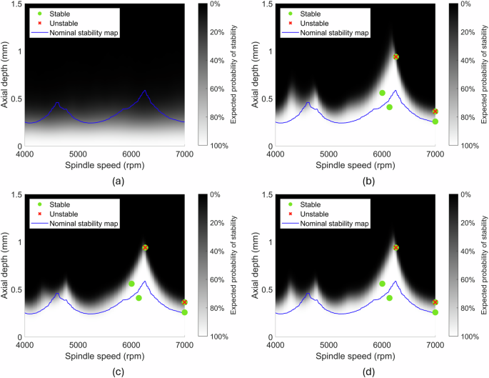
The list of selected test cuts is shown in Table 2. Bayesian updating was performed using these test cuts, both with and without using spindle power learning. Figure 13 shows the prior and posterior stability maps compared to the nominal stability boundary calculated using the ZOA stability algorithm. This example identified the stability peak in only three recommended test cuts (six total cuts since each cut was run at two feed rates), and there is no significant difference between the two different posterior stability maps.

a Prior. b Posterior without spindle power learning. c Posterior with spindle power learning.
While using spindle power did not significantly affect the stability map, it did help the model learn the tangential cutting force model. Table 3 compares the prior and posterior uncertainties for the two cases. Including the spindle power in the updating reduced uncertainty for both ({k}_{{te}}) and ({k}_{{tc}}), but did not significantly lower the ({k}_{{nc}}) or (beta) uncertainties. Additionally, the lower cutting force uncertainty reduces the stiffness uncertainty, since the limiting axial depth is determined by both the cutting force and stiffness.
The model also learns to accurately predict the spindle cutting power, even for tests where the spindle power was not used for learning. Figure 14 compares the 1σ probabilistic predictions for the spindle power for each cut before and after the cutting test series was run. Both the prior and no power learning cases significantly overestimate the spindle power for each test, largely due to the high prior estimate for ({k}_{{te}}). When spindle power was incorporated in the learning process, however, the Bayesian model accurately predicts the power requirements for each cut. Note that the spindle power model presented in Section “Physics models and probabilistic simulation” does not perfectly match the time domain power simulations. The green dots show that model’s nominal predictions for the spindle power for each cut. Severe chatter was encountered during test 1 ((M=) 155 μm at 0.1 mm feed rate) which caused the tool to disengage with the workpiece, reducing the power requirements. Test 2 also experienced chatter but had less error since the chatter had lower amplitude ((M=) 29 μm at 0.1 mm feed rate). The stable cuts also are not perfectly accurate since the spindle power model ignores tool deflection and vibration, but the predictions are generally close to the simulated values.

For the prior and no power cases, the error bars indicate the epistemic uncertainty. For the ({sigma }_{P}=) 20 W case, the inner error bars indicate epistemic uncertainty while the outer error bars indicate the combined epistemic and aleatoric uncertainty.
Experimental study
An experimental case study was performed to validate the model and demonstrate how it accommodates uncertainty in the physics algorithms. It builds on the results presented in ref. 41. Cutting tests were performed on a 1080 mild steel workpiece on a vertical machining center. The audio and spindle power were recorded for each test cut. Specific details on the experiments and measurements are found in Section “Experimental study”. Table 4 lists the settings for the Bayesian model. The stability aleatoric uncertainty was set higher than during the numerical study since the tool had a 2 mm corner radius which can shift the stability boundary.
The prior uncertainties were set manually and intended to reflect a worst-case scenario case where the user has very little information about the machining system and has not performed any measurements for the cutting forces or dynamics. The cutting force prior is set based on author’s experience machining steel, and in this case, significantly underestimates the true cutting forces. The dynamics prior is set as a uniform distribution which assumes the system has two modes with natural frequencies between 1000 and 2000 Hz and similar stiffness and damping, but otherwise provides no information about the modes. However, if the priors for both modes are identical then the Bayesian algorithm will find two solutions for the model, one where ({f}_{n1} ,>, {f}_{n2}) and another where ({f}_{n1} ,<, {f}_{n2}). To avoid this, the prior was multiplied by the penalty function shown in Eq. 30, which constrains the system such that ({f}_{n1}ge {f}_{n2}). See Table 6 for the full prior along with the posterior distributions.
First, a series of test cuts were selected and performed without using the spindle power in the Bayesian updating. As with the numerical study, cutting tests were performed at two feed rates to effectively learn both the cutting and edge force coefficients. Initially, tests were selected using the MRR maximizing algorithm. However, after the first two selected test points (four total test cuts at different feed rates) the MRR maximizing algorithm was unable to suggest a new test due to high ({f}_{n1}) uncertainty. While ({f}_{n2}) was identified by observing the chatter frequency, ({f}_{n1}) was not observed and the algorithm must infer ({f}_{n1}) from the fact that ({f}_{n2}) has a lower limiting axial depth at 7000 rpm, resulting in a complex multimodal distribution as shown in Fig. 15. Since there is no clear stability peak, the MRR maximizing algorithm cannot recommend a new test. Therefore, the next cutting test was selected to reduce uncertainty in ({f}_{n1}). After this, the algorithm was confident enough about the location of the stability peak to switch back to MRR maximization until the stopping criteria was met. Table 5 shows the final test cut series.

a Probabilistic stability map. b Distribution of natural frequencies.
Next, updating was performed using the same series of test cuts including the measured spindle power in the likelihood function. Since the same series of test cuts are used, this establishes how the spindle power measurement helps learn the cutting force model. Two different power uncertainties were used: a low uncertainty case with ({sigma }_{bar{P}}=) 5 W based on the noise in the power measurement, and a high uncertainty case with ({sigma }_{bar{P} % }=) 25% based on the uncertainty of the power prediction. When combined with no spindle power measurement, these three cases give the posterior probabilistic stability maps shown in Fig. 16. Note that they all converged to similar stability predictions.
a Prior. b Posterior with no spindle power learning. c Posterior with low uncertainty spindle power learning. d Posterior with high uncertainty spindle power learning with high uncertainty.
Table 6 shows the prior and posterior distributions for each case. The posterior distributions are calculated by calculating the mean and standard deviation of the samples drawn using the MCMC method. The nominal values for the tool dynamics and force model were measured using modal tap testing and cutting force dynamometer tests, respectively. The no-spindle power case underestimates ({k}_{{tc}}) by 44%. This is because the true stability limit is significantly higher than predicted by the ZOA algorithm, causing the Bayesian algorithm to increase the system stiffness and decrease the cutting force to compensate. This inaccuracy in the nominal prediction is likely due to approximations in the ZOA model. First, the ZOA does not consider the tool’s 2 mm corner radius. Due to that corner radius, the actual engagement and forces between the tool and workpiece are lower than expected. Second, the ZOA ignores process damping, where vibrational energy is dissipated due to interference between the tool and workpiece as they vibrate relative to each other42. Both these factors can cause the ZOA to underestimate the true stability limit.
Furthermore, the no-spindle power case entirely failed to learn the edge coefficient ({k}_{{te}}) since it has no effect on stability or chatter frequency. In contrast, the low uncertainty power case accurately learned ({k}_{{tc}}) and ({k}_{{te}}). However, the posterior for the system stiffness is less accurate than the original. When the spindle power is measured, the cutting force cannot be artificially decreased to raise the stability limit, so the stiffness must be increased further. The high uncertainty case was between the other cases. The high uncertainty for the power allowed the Bayesian algorithm to artificially decrease the power, albeit not as much as when power was omitted entirely.
None of the cases accurately identified ({f}_{n1}) since no chatter frequency was observed for that mode. This could occur either because every test cut could have lined up with a stability peak, or because mode 1 could be much stiffer than mode 2 such that it has a higher limiting axial depth even at its stability troughs. In this case, the second scenario is correct, where mode 1 is 3.8 times stiffer than mode 2. However, the prior assumes that both modes have similar stiffnesses and therefore finds a natural frequency that aligns the stability peak with the tests. The spindle speed for the (j) th stability peak for some given natural frequency can be calculated using Eq. 31. For a natural frequency of 1648 Hz the 5th stability peak occurs at roughly 6600 rpm, allowing it to plausibly encompass all the test cuts.
While the low power uncertainty case learned the cutting force coefficients, it was not able to accurately predict the cutting test results due to high uncertainty in the power predictions themselves. Figure 17 compares the measured power and nominal predictions based on the measured cutting force coefficients to the probabilistic power predictions for each case. On average, there is a 25% absolute deviation between the measured spindle power and the nominal prediction for each test cut, with different cases both over and underestimating the power. This error is significantly larger than the numerical case study due to the 2 mm corner radius on the tool. The cutting force model presented in Section “Physics models and probabilistic simulation” assumes that the tool has a square corner and thus does not accurately predict the spindle power in all cases. The low uncertainty case is not able to accommodate this model uncertainty and confidently predicts a narrow range of possible values for each test, often not including the true value. In contrast, the high uncertainty case captures the full range of test outcomes, with six of the 10 test cuts appearing within the 1σ 68% confidence interval.

For the prior and no power learning cases, the error bars show the 1σ epistemic uncertainty for the power. For the cases with spindle power learning, the inner error bars represent the 1σ epistemic uncertainty, while the outer error bars show the combined epistemic and aleatoric uncertainty.
Discussion
The case studies demonstrate how the Bayesian model can be extended to include other predictions and inputs. Incorporating the chatter frequency and measured spindle power helps learn the true tangential cutting force model and system natural frequency from a small number of cutting tests, which is not possible when using only binary stable/unstable test results. Cutting tests can also be selected to provide maximum information about the underlying system, allowing the user to reduce uncertainty as quickly as possible. However, other parameters like the normal force model, stiffness, and damping are relatively difficult to learn through test cuts. The normal cutting forces have little effect on stability or spindle power and thus cannot be directly obtained from the data collected in this study. The stiffness can be inferred from the limiting axial depth, but determining this accurately requires many cutting tests and is susceptible to bias from physics model assumptions. In the future, this could be resolved by incorporating additional signals to the Bayesian updating, for example, the axis drive currents or measured surface location error.
In addition to identifying system parameters, the Bayesian approach can make probabilistic predictions about test outcomes such as the spindle cutting power. Incorporating both epistemic and aleatoric uncertainty into the predictions accommodates uncertainty in measurements and physics models and establishes reasonable uncertainty bounds, even when there is high model uncertainty as in the experimental case study. This is critical for safe test selection since it can allow users to fully understand the risks associated with performing a given test cut, e.g., to allow test selection to be constrained based on the machine tool’s available spindle power.
However, this method of incorporating model assumptions into the aleatoric uncertainty has some limitations. First, it assumes that physics uncertainties are normally distributed and cannot account for consistent bias in predictions. This can result in skewed predictions for the system parameters, e.g., in the experimental case study where the ZOA algorithm consistently underpredicted the stability limit. Furthermore, because the Bayesian model is solely physics-based, the assumptions of the physics algorithm constrain its predictions. For example, in the experimental case study, the stability boundary depended on feed rate, but since the ZOA algorithm assumes that stability is independent of feed it fits an approximate stability boundary to both results. Similarly, unlike more general machine learning algorithms (e.g., neural networks), the model uncertainty cannot be reduced as more tests are added, as shown in the experimental case study where there was significant uncertainty about the power prediction for a given test even after it has already been performed and observed. Future work can investigate new ways to model or reduce bias, for example by incorporating more accurate machining simulations (e.g., high-accuracy time domain simulations43 with non-linear cutting force models44 and process damping42), automatically learning the aleatoric uncertainty from the test cut results by incorporating ({sigma }_{bar{P}}) into the (theta) vector, incorporating learnable bias terms separate from the likelihood function, and automatically learning the aleatoric uncertainties from test results.
Methods
This section describes details of the experimental verification necessary to replicate the verification studies. Both studies used the Bayesian updating model described in Section “Prior definition” through “Markov Chain Monte Carlo sampling” to iteratively select test cuts and update the prior distribution of system parameters, repeating until the stopping criteria were reached. Full MATLAB code for both case studies is available on GitHub under an MIT license: see the Code Availability Statement at the end of this article. A brief introduction to the codebase and detailed descriptions on implementation and optimization can be found in ref. 41. The remainder of this section describes specific experimental details for each study.
Numerical study
The numerical study simulated a three flute 12.7 mm diameter endmill cutting an aluminum workpiece using climb (down) milling. Each test was simulated using time domain simulation1. This approach estimates the instantaneous cutting forces on the tool at discrete timesteps. The cutting force is calculated using the mechanistic force model based on the current engagement between the tool and workpiece, factoring in the current vibrational displacement of the tool. Those forces are then used to estimate the vibration of the tool at the next timestep estimated using Euler integration. This process is repeated until the desired simulation length has been achieved, at which point the simulated displacements and cutting forces can be analyzed. The simulation used a timestep of 1/30,000th of a second and was run for 100 tool revolutions (e.g., if the tool was rotating at 100 rotations per second then the simulation would run for one second and have 30,000 total timesteps). These settings were selected to provide sufficient temporal resolution to fully capture the tool vibration while having enough length to reach steady-state vibration. The time domain simulation function is included in the published MATLAB code.
Each time domain simulation was classified as stable or unstable using the periodic sampling (M)-metric shown in Eq. 32 with a cutoff of (M=) 1 μm45. In that formula, ({N}_{s}) is the total number of once-per-rev samples drawn from the signal and ({x}_{s}(i)) is the (i) th displacement sample. This approach samples from the tool’s displacement signal once-per revolution and calculates the average absolute difference between subsequent samples. In stable cuts, the tool experiences forced vibration which repeats with every flute pass, resulting in a low (M) value. Unstable cuts show variation from flute to flute and have high (M) values, indicating that the tool is experiencing self-excited vibration. Figure 18 compares the simulated deflections for stable and unstable milling conditions. In Fig. 18a the once-per-revolution samples in the stable cut repeat nearly perfectly every revolution. This indicates that the tool is experiencing forced vibration, and the cut is therefore classified as stable. In contrast, Fig. 18b shows a case where self-excited vibrations cause the tool to vibrate at a frequency which is not a harmonic of the flute passing frequency. As a result, the once-per-revolution samples do not repeat and the cut is classified as unstable.

a Stable cut. b Unstable cut. Red dots show the once-per-revolution samples used to calculate the (M)-metric.
Experimental study
In the experimental case study, test cuts were performed on a vertical machining center to demonstrate the proposed framework. Table 7 details specific testing conditions. Each test was recorded using a microphone located inside of the machine enclosure to obtain the chatter frequency and help classify the test stability. Spindle power was measured using a Rogowski coil setup to measure the spindle motor current and voltage. Figure 19a, b shows the microphone and Rogowski coil setups inside of the machine tool. For each test, the spindle cutting power was calculated by subtracting the average power before the tool entered the cut from the average steady-state power during the machining cut, as shown in Fig. 19c.
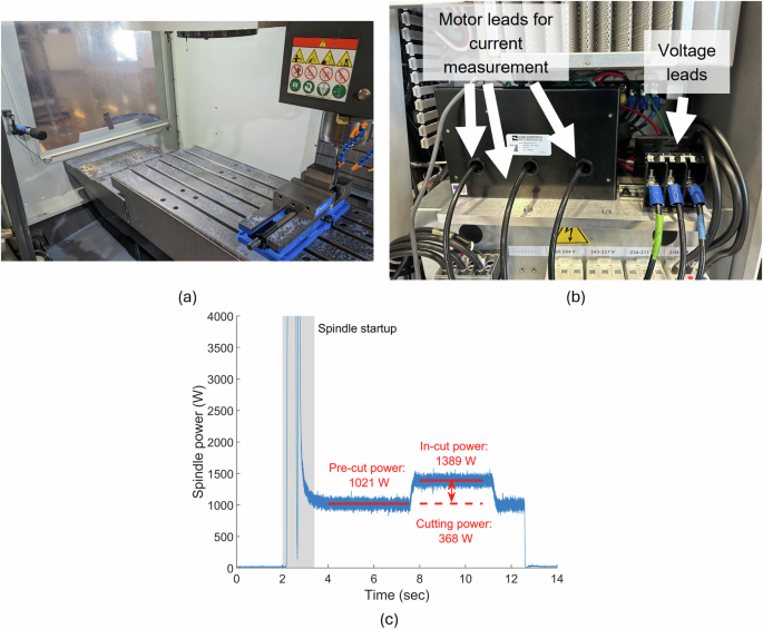
a Testing setup in the machine. b Rogowski coil setup in the machine tool cabinet to measure spindle voltage and current. c Spindle power measurement for test #4 at 0.06 mm feed.


Responses