Antibiotic susceptibility testing using minimum inhibitory concentration (MIC) assays

Antibiotic resistance is a major threat to global health. Resistant bacterial infections are currently resulting in over 1.2 million deaths every year¹ and are projected to reach 10 million casualties annually by 2050. This crisis is due to the continuous emergence and spread of antibiotic-resistance genes across important human pathogens and the limited introduction of new, broad-acting, clinically useful antimicrobials since the 1970s². Alongside genetic resistance, alternative bacterial lifestyles during infection, such as persistence³ and growth in biofilms⁴, also contribute to patient mortality due to ineffective antibiotic treatment. As such, it has become essential to not only boost our currently insufficient preclinical and clinical antimicrobial development pipelines⁵ but to also safeguard the longevity of our approved antibiotics. Both feats heavily rely on our ability to evaluate the efficacy of antimicrobial agents against bacteria, which underpins the identification of antibiotic-resistant strains in the clinic and enables testing of novel antibiotic or antibiotic-adjuvant candidates.

The minimum inhibitory concentration (MIC) assay is the gold standard for determining the susceptibility of a bacterial strain to an antimicrobial molecule of interest. Briefly, to perform a MIC assay, a pure culture of the tested bacterial strain is standardized to 5 × 10⁵ colony forming units (CFU)/mL^6,7 and exposed to a range of antibiotic concentrations at 37 °C for 16–24 h (for some organisms and MIC determination methods the incubation times may vary⁸). After this incubation period, bacterial growth is assessed for each antibiotic concentration, and the MIC value is identified as the lowest concentration of the antimicrobial molecule required to inhibit visible growth of the tested strain.

MIC assays are routinely performed in clinical laboratories to assess the antimicrobial susceptibility of bacterial infections. For this purpose, clinical breakpoints have been developed for approved antibiotics, and denote the MIC values below which an infection is likely to be highly treatable. As such, clinical breakpoints can be used by clinicians in conjunction with empirical evidence to help determine a suitable antibiotic treatment plan. Clinical breakpoints help inform treatment efficacy by considering the pharmacokinetics and dosing regimen of a given antimicrobial, the infecting organism, and the location of the infection. In particular, a comparison of the recorded MIC value to published clinical breakpoints⁹ designates a bacterial strain of interest as susceptible (sensitive, likely treatable at normal dosing regimen) or resistant (non-sensitive, untreatable) to a particular antimicrobial agent. In addition to this binary classification that applies to some organisms, some bacterial species may instead fall into an ‘intermediate / susceptible at increased exposure’ category, whereby treatment with an antimicrobial agent may be possible, but requires further consideration with respect to dosing regimen, infection type, infection location, or previous patient exposure¹⁰.

Beyond diagnostic laboratories, MIC determination in research laboratories serves as a method commonly employed to study antibiotic-resistance mechanisms, identify new drug targets, and assess the promise of novel drug candidates. The use of standardized MIC assay guidelines stemming from clinical practice in research environments allows rapid and meaningful data interpretation, easy cross-comparison of results between different research groups, and acquisition of clinically translatable results^11,12.

Both clinical breakpoints and antibiotic-specific MIC assay standards are regularly reviewed by several international bodies. The two most commonly recognized organizations are the Clinical & Laboratory Standards Institute (CLSI)⁷ and the European Committee on Antimicrobial Susceptibility Testing (EUCAST)⁹. Although the use of instructions from both health standard bodies is recommended by the World Health Organization¹³, there are significant variations within their respective methods and assessment guidelines^14,15,16. Notably, there are differences even in the definitions of the resistance categories described above, which can become challenging or confusing for researchers and clinicians relying on the use of MIC assays. For example, in the case of the antibiotic fosfomycin, strains with identical MIC values can be classified as resistant or susceptible, depending on the health standard body guidelines used¹⁷. Due to these variations and yearly guideline updates, it is critical that the most current recommendations for MIC protocols and clinical breakpoint values are consulted regularly. Laboratory assays should be updated as necessary prior to performing MIC experiments or assessing the obtained results. It is also important to include the assessment system that was used (EUCAST, CLSI, or other) and the year or version of the guidelines adhered to when reporting on MIC values and susceptibility phenotypes.

Finally, MIC assays are commonly validated using quality control strains with well-characterized genotypes and stable resistance mechanisms. These controls are bacterial-species- and antibiotic-agent-specific and may vary between laboratories. Recommended quality control strain examples can be found in the EUCAST quality control tables and the CLSI ‘M100-ED34:2024 Performance Standards for Antimicrobial Susceptibility Testing, 34th Edition’ document^7,18.

For clarity, all recommendations and results discussed in this methods paper are based on the more widely available EUCAST guidelines and are valid as of January 2024. The links to these guidelines and other supporting documents are available in Supplemental File 1; directions on how to access the corresponding CLSI documents are included for comparison purposes. The protocols described in this methods paper are intended for research purposes only and do not serve as an official guide for clinical microbiology laboratories.

We describe two standard EUCAST-based methods that can be employed for the determination of antibiotic MIC values for non-fastidious organisms⁶.

These methods involve using:

• i) commercial antibiotic gradient strips (Protocol 1)

• ii) liquid broth microdilution (Protocol 2a).

We also include two modifications of the broth microdilution method to describe its use in:

• i) cation-adjusted MIC determination for polymyxin antibiotics, like colistin (Protocol 2b)

• ii) low-volume MIC determination to be used for cases where limited amounts of test compounds, such as antimicrobial peptides, are available (Protocol 2c).

All steps in the described protocols should be carried out in a suitable BSL-class laboratory using sterile conditions to prevent health risks and contamination. For research purposes, we recommend that each strain of interest is tested in biological triplicate and performed on different days to ensure reproducibility¹¹. Even though it would increase the reliability of the obtained results, this practice is not usually applied in clinical laboratories, whereby MIC assays are performed in a single biological replicate¹¹. Single technical replicates are acceptable for MIC assessment using commercial antibiotic gradient strips (Protocol 1) unless otherwise stated by the antibiotic gradient strip manufacturer. Technical replicates in triplicate should be performed for all liquid broth dilution methods (Protocols 2a/2b/2c).

Representative experiments and results for Protocols 1 and 2a are shown using the β-lactam antibiotic ceftazidime against a panel of susceptible and resistant Escherichia coli MC1000 strains (Table 1). Representative experiments for Protocol 2b are shown using colistin against a panel of susceptible and resistant E. coli W3110 strains (Table 1). For simplicity, we include the E. coli ATCC 25922 strain, recommended by EUCAST, as the sole quality control strain in the representative experiments showcased here. Required materials for Protocols 1 and 2 are listed in Tables 2 and 3, respectively.

The following steps are common to both protocols described in this paper:

Bacterial strain growth:

Day 1.

1. 1.1

   Using a sterile 1 μL loop, streak out all strains to be tested on LB agar (or similar rich medium; supplement with an appropriate antibiotic selection, if required).

2. 1.2

   Incubate statically overnight at 37 °C.

Day 2.

1. 1.3

   Using a sterile 1 μL loop, inoculate a 5 mL overnight culture of LB broth (or similar rich medium; supplement with an appropriate antibiotic selection, if required) with a single colony of each strain to be tested.

2. 1.4

   Incubate overnight at 37 °C with agitation at 220 RPM.

Inoculum preparation:

1. 1.1

   Gently mix the overnight cultures using a vortex.

2. 1.2

   Mix 100 μL of the overnight culture with 900 μL of growth media. Transfer the mixture into a UV-Vis cuvette and measure the OD600 using a spectrophotometer.

3. 1.3

   Calculate the volume (μL) of the overnight culture needed to prepare the standardized inoculum using the following formula:

   $$begin{array}{l}{rm{Volume}}left({rm{mu L}}right){{rm{of}}; {rm{overnight}}; {rm{culture}}; {rm{required}}; {rm{to}}; {rm{make}}},1;{{rm{mL}}; {rm{of}}; {rm{OD}}}600,{{rm{standardized}}; {rm{innoculum}}}\ =1000,{{upmu {rm{L}}}}div(10times {rm{OD}}600,{rm{measurement}})/({{rm{target}}; {rm{OD}}}600)end{array}$$

   (1)
4. 1.4

   Pipette the required volume of the overnight culture (determined from Eq. 1) into a sterile 1.5 mL microtube. Add 0.85% w/v sterile saline solution up to 1 mL. This is your inoculum.

5. 1.5

   Use the inoculum within 30 minutes of preparation.

CFU enumeration: This should be performed at least once per bacterial strain.

For Protocol 1, check your inoculum by performing a serial dilution from 10⁻¹ to 10⁻⁶ of the inoculum. Prepare the first dilution (10⁻¹) by mixing 100 μL of the inoculum into 900 μL 0.85% w/v sterile saline solution; then repeat this step 6 times to reach the 10⁻⁶ dilution. Plate out 3 × 20 µL spots per dilution on a non-selective agar medium. Incubate the plates statically for 18–24 h at 37 °C. The next day enumerate the single colonies. The inoculum should be ~5 × 10⁵ CFU/mL.

For Protocols 2a/2b/2c, check your inoculum by diluting 10 µL of the positive growth-control wells (Fig. 2, row ‘G’) in 10 mL of 0.85% w/v sterile saline and plating 100 µL on a non-selective agar medium. Incubate the plates statically for 18–24 h at 37 °C. The next day enumerate the single colonies. The inoculum should be ~5 × 10⁵ CFU/mL.

Protocol 1. MIC determination using antibiotic gradient strips

Follow the ‘Bacterial strain growth’ instructions for Days 1 and 2.

Day 3.

Mueller–Hinton agar plate preparation:

1. 1.1

   Prepare Mueller–Hinton Agar plates, and supplement with an inducer if required. No antibiotics should be added to these plates. Standard 100 mm Petri dishes accommodate up to two antibiotic gradient strips; you will need ~15 mL of Mueller–Hinton agar per plate. Large 150 mm Petri dishes accommodate up to five antibiotic gradient strips; you will need ~65 mL of Mueller–Hinton agar per plate.

   Note: Inducers, such as Isopropyl β-d-1-thiogalactopyranoside (IPTG) or l-arabinose, should only be included during this step in experiments where the tested strains harbor synthetic, inducible plasmids.

2. 1.2

   Dry the Mueller–Hinton agar plates by leaving them open to air under sterile conditions for 5–10 min.

Inoculum preparation:

1. 1.3

   Prepare the standardized inoculum at OD600 = 0.063 in 0.85% w/v sterile saline as per Eq. 1 in ‘General Methods, Inoculum preparation’.

MIC assay:

1. 1.4

   Dip a sterile cotton-tipped applicator into the inoculum and evenly spread the suspension onto the Mueller–Hinton agar surface. Spread three times, in overlapping directions, dipping into the inoculum between each application. Allow a few minutes so that the inoculum dries fully. For 150 mm Petri dishes, dip into the inoculum twice per application direction.

2. 1.5

   Use sterile tweezers (or flame-sterilize the utensil) to place the antibiotic gradient strips on the agar at an even distance. See Fig. 1 for how to space the antibiotic gradient strips on the plates.

   

   A A single colony is incubated overnight in 5 mL of rich media with appropriate antibiotic selection. B OD600 of the overnight culture is measured. C Standardized inoculum at OD600 = 0.063 is prepared in 0.85% w/v sterile saline solution. D Bacteria are spread evenly across a Mueller–Hinton agar plate to create a thin lawn. E Antibiotic gradient strips are distributed evenly on the plate. Standard 100 mm Petri dishes fit one (right) or two (middle) strips. Larger, 150 mm, Petri dishes can accommodate up to 5 strips (left). F Plates are statically incubated at 16–24 h at 37 °C. The MIC is determined at the intersection of the gradient antibiotic strip and the zone of inhibition (bacterial growth is depicted in pink and the zone of inhibition in light blue) and is denoted by the red arrows. Figure created in BioRender; Kaderabkova, N. (2023).

   Full size image

3. 1.6

   Use tweezers to gently tap the top of the strip from the lowest to the highest concentration to secure it onto the Mueller–Hinton agar surface. Take care not to displace the strip.

4. 1.7

   Incubate the plates upside down (lid down) statically for 16–24 h at 37 °C.

   Note: Incubation time depends on the bacterial species and, potentially, also on the gradient test manufacturer; always consult manufacturer instructions. If no instructions are given, the bioMérieux E-test application guide may be a good starting point⁸.

Day 4.

1. 1.8

   Record MIC values at the antibiotic gradient strip and growth inhibition zone intersection.

Protocol 2a. MIC determination using broth microdilution

Follow the ‘Bacterial strain growth’ instructions for Days 1 and 2.

Day 3.

96-well plate preparation:

1. 1.1

   Prepare the highest concentration of the antibiotic to be tested in Mueller–Hinton broth, and supplement with an inducer if required. You will need ~300 µL of antibiotic solution for each top-row well + ~10% extra volume to allow for accurate pipetting. No additional antibiotics beyond the tested compound should be added.

   Note: (a) Although it is often deemed insignificant and not taken into consideration, preparation of the solution with the highest antibiotic concentration should account for the addition of 5 μL of inoculum described in step 1.7 of this protocol. The addition of 5 μL into a total volume of 150 μL corresponds to a 3.3% nominal decrease in concentration, therefore the concentration of the antibiotic stock should be 3.3% higher than the desired highest antibiotic concentration.

   (b) We suggest that the antibiotic stock is made fresh each time to prevent any changes in concentration due to freezing and thawing. Inducers, such as IPTG or l-arabinose, should only be included during this step in experiments where the tested strains harbor synthetic, inducible plasmids.

2. 1.2

   Using a pipette, aliquot 300 µL of the highest concentration antibiotic solution into the top wells of the 96-well plate (Fig. 2, row ‘A’).

   

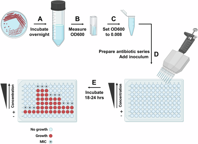
   A A single colony is incubated overnight in 5 mL of rich media with appropriate antibiotic selection. B OD600 of the overnight culture is measured. C Standardized inoculum at OD600 = 0.008 is prepared in 0.85% w/v sterile saline solution. D Antibiotic concentration gradient is created in Mueller–Hinton broth in a 96-well plate, such that the top row of the plate (row ‘A’) contains the highest antibiotic concentration, and the concentration decreases in the rows below (rows ‘B’–‘F’) by twofold each time. The last two rows (rows ‘G’ and ‘H’) contain antibiotic-free Mueller–Hinton broth and act as the positive (‘+’) and negative (‘–‘) growth-control wells. The positive (‘+’) growth-control wells report on the bacterial strain viability in the conditions of the MIC assay, while the negative (‘–‘) growth-control wells report on growth media contamination. The inoculum is added into each well of the plate, except the negative control well. E The 96-well plate is incubated for 16–24 h at 37 °C. The MIC is determined as the lowest concentration for which there is no visible bacterial growth (bacterial growth is indicated by red color, no growth is indicated by light blue color, and the MIC wells are labeled with a star on the left 96-well plate schematic). Figure created in BioRender; Kaderabkova, N. (2023).

   Full size image

3. 1.3

   Using a multichannel pipette (P150–P300), aliquot 150 µL of antibiotic-free Mueller–Hinton broth (supplemented with an inducer, if required), into all the other wells of the plate.

4. 1.4

   Use a multichannel pipette (P150–P300) to remove 150 µL of antibiotic solution from the top-row wells (Fig. 2, row ‘A’) and mix with the antibiotic-free Mueller–Hinton broth in the wells of the next row (row ‘B’). Pipette up and down gently several times to mix the new antibiotic concentration. Discard the tips.

5. 1.5

   Continue in this manner until the lowest concentration of antibiotic is achieved (Fig. 2, row ‘F’). Then discard 150 µL of solution from the wells with the lowest concentration of antibiotic. Make sure not to add any antibiotic into the positive or negative growth-control rows (Fig. 2, rows ‘G’ and ‘H’).

   Inoculum preparation:

6. 1.6

   Prepare the standardized inoculum at OD600 = 0.008 in 0.85% w/v sterile saline as per Eq. 1 in ‘General Methods, Inoculum preparation’.

   MIC Assay:

7. 1.7

   Using a multichannel pipette (P10), add 5 µL of inoculum into each well of the antibiotic series (Fig. 2, rows ‘A’–‘F’) and into the positive growth-control row (Fig. 2, row ‘G’). This results in a final bacterial load of ~5 × 10⁵ CFU/well. Do not add any inoculum to the negative growth-control row (Fig. 2, row ‘H’).

8. 1.8

   Incubate the 96-well plate statically for 16–24 h at 37 °C.

   Day 4.

9. 1.9

   Record the MIC values by visual inspection. The MIC is the lowest antibiotic concentration, with no visible (by the naked eye) growth of bacteria in the well. The MIC value is the consensus, not the average, of the three technical replicates.

Protocol 2b. MIC determination using broth microdilution—modification for colistin MIC value determination

All colistin MIC assays should be run in cation-adjusted Mueller–Hinton media to decrease MIC value variability. This can be either commercially sourced or cations can be supplemented in regular Mueller–Hinton medium in the form of CaCl₂ and/or MgCl₂. The EUCAST guidelines recommend solely the use of the broth microdilution method for colistin MIC determination¹⁹, while CLSI also allows for the use of agar dilution and broth disk dilution methods⁷ (not discussed as part of this methods paper).

Follow the ‘Bacterial strain growth’ instructions for Days 1 and 2.

Day 3.

96-well plate preparation:

1. 1.1

   Prepare a colistin sulfate stock solution at 2 mg/mL in cation-adjusted Mueller–Hinton, and supplement with an inducer, if required, in a small (~50 ml) glass beaker. Ensure that all colistin has dissolved using a small metallic spatula.

   Note: We suggest that the antibiotic stock should be made fresh each time to prevent any changes in concentration due to freezing and thawing. The use of glass containers is preferred to minimize the loss of colistin concentration due to adhesion to plastic surfaces. Inducers, such as IPTG or l-arabinose, should only be included during this step in experiments where the tested strains harbor synthetic, inducible plasmids.

2. 1.2

   Prepare all the desired colistin concentrations in cation-adjusted Mueller–Hinton broth (supplement with an inducer if required) in glass 100 mm Petri dishes. You will need ~150 µL antibiotic solution for each well + ~20% extra volume to allow for accurate pipetting. Plastic Petri dishes may be used if no glass plates are available. However, contact with the colistin solutions should be kept to a minimum. No additional antibiotics beyond colistin should be added.

   Note: As described in Protocol 2a, each desired colistin concentration should be nominally increased by 3.3% to account for the 5 µL inoculum addition.

3. 1.3

   Using a multichannel pipette (P150–P300), aliquot 150 µL of each of the antibiotic concentrations into the corresponding rows of the 96-well plate (Fig. 2, rows ‘A’–‘F’). Discard tips after each use. If the solution is taken up incorrectly by the multichannel (e.g., air bubbles are present, or the tip is leaking), discard the tips and the antibiotic solution; the contact of colistin with laboratory plastics should be kept to a minimum.

4. 1.4

   Using a multichannel pipette (P150–P300), aliquot 150 µL of antibiotic-free cation-adjusted Mueller–Hinton broth (supplemented with an inducer if required), into the positive and negative growth-control rows (Fig. 2, rows ‘G’ and ‘H’).

Follow Protocol 2a from the ‘Inoculum preparation step’ on Day 3.

Protocol 2c. MIC determination using broth microdilution—modification for low-volume MIC assays

This protocol is helpful for testing the efficacy of compounds for which limited amounts are available to the user, for example, antimicrobial peptides. It should be noted that the technique for preparing the antibiotic solutions and inoculum described here could also be used in Protocols 2a and 2b if adjusted to achieve a final volume of 150 μL per well.

Follow ‘Bacterial strain growth’ instructions for Days 1 and 2.

Day 3.

96-well plate preparation:

1. 1.1

   Prepare a solution containing 2× the highest desired concentration of the tested antimicrobial compound in Mueller–Hinton broth, and supplement with an inducer if required. You will need ~100 µL of antimicrobial compound solution for each top-row well + ~10% extra volume to allow for accurate pipetting. No additional antibiotics beyond the tested compound should be added.

   Note: We suggest that the antimicrobial compound stock is made fresh each time to prevent any changes in concentration due to freezing and thawing. Inducers, such as IPTG or l-arabinose, should only be included during this step in experiments where the tested strains harbor synthetic, inducible plasmids.

2. 1.2

   Aliquot 100 µL of the 2× highest concentration antimicrobial compound solution into the top wells of the 96-well plate.

3. 1.3

   Using a multichannel pipette (P150), aliquot 50 µL of compound-free Mueller–Hinton broth (supplemented with an inducer, if required), into all the other wells of the concentration gradient (Fig. 2, rows ‘B’–‘F) and into the positive growth-control row (Fig. 2, row ‘G’).

4. 1.4

   Using a multichannel pipette (P150), aliquot 100 µL of compound-free Mueller–Hinton broth (supplemented with an inducer, if required), into the negative growth-control row (Fig. 2, row ‘H’).

5. 1.5

   Use a multichannel pipette (P150) to remove 50 µL from the top-row wells (Fig. 2, row ‘A’) and mix with the compound-free Mueller–Hinton broth in the wells of the next row (row ‘B’). Pipette up and down gently several times to mix the new antimicrobial compound concentration. Discard the tips.

6. 1.6

   Continue in this manner until the lowest concentration of antimicrobial compound is achieved (Fig. 2, row ‘F’). Then discard 50 µL of solution from the wells with the lowest concentration of antimicrobial compound. Make sure not to add any antimicrobial compound into the positive or negative growth-control rows (Fig. 2, rows ‘G’ and ‘H’).

Inoculum preparation:

1. 1.7

   Prepare the standardized inoculum at OD600 = 0.002 in 0.85% w/v sterile saline as per ‘General Methods, Inoculum preparation’.

MIC Assay:

1. 1.8

   Using a multichannel pipette (P150), add 50 µL of the inoculum into each well of the antimicrobial compound series (Fig. 2, rows ‘A’–‘F’) and into the positive growth-control row (Fig. 2, row ‘G’). This results in a final bacterial load of ~5 × 10⁵ CFU/well. Do not add any inoculum to the negative growth-control row (Fig. 2, row ‘H’).

2. 1.9

   Incubate the 96-well plate statically for 16–24 h at 37 °C. The time of incubation is species and antimicrobial compound specific.

   Day 4.

3. 1.10

   Record the MIC values by visual inspection. The MIC is the lowest antimicrobial compound concentration, with no visible (by the naked eye) growth of bacteria in the well. The MIC value is the consensus of the three technical replicates.

MIC values are standardly expressed as mg/L or µg/mL and refer to the lowest concentration of an antimicrobial agent required to prevent visible growth of a specific bacterial strain in vitro. A rule of thumb is that potent antibiotic compounds are associated with low MIC values, while weak antimicrobials result in high MICs. Here, we provide general guidance on the interpretation of MIC values obtained using antibiotic gradient strips and the broth microdilution method. Detailed guidance, specific to each antibiotic, is provided by EUCAST, CLSI, and antibiotic manufacturers, and should be consulted as necessary when MIC assays are performed (see Supplemental File 1 for useful links).

Using Protocols 1, 2a, and 2b we determined the MIC values for ceftazidime and colistin antibiotics for a panel of E. coli strains (Table 4 and Fig. 3). E. coli ATCC 25922 was used as the quality control strain for both protocols.

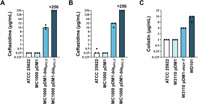
A Ceftazidime (β-lactam antibiotic) MIC values were determined using a commercial antibiotic gradient strip (Protocol 1) for the quality control strain (E. coli ATCC 25922), an experiment-specific empty-vector control strain (E. coli MC1000 pDM1), and two β-lactamase-expressing strains (E. coli MC1000 pDM1-bla_KPC-2 and E. coli MC1000 pDM1-bla_KPC-3). The clinical breakpoint for ceftazidime is at MIC > 4 μg/mL by EUCAST⁹ and MIC ≥ 16 μg/mL by CLSI²⁰. MIC determination was carried out in biological triplicate, as a single technical repeat. B Ceftazidime MICs were determined using the broth microdilution method (Protocol 2a) for the same bacterial strains as in panel (A). MIC determination was carried out in technical and biological triplicate. C Colistin (polymyxin antibiotic) MICs were determined using the broth microdilution method adapted for colistin (Protocol 2b) for the quality control strain (E. coli ATCC 25922), an experiment-specific empty-vector control strain (E. coli W3110 pDM1), a strain harboring a mobile colistin resistance gene on a plasmid (E. coli W3110 pDM1-mcr-1), and a strain that is resistant to colistin through a chromosomal mutation (E. coli WD101²²). The clinical breakpoint for colistin is at MIC > 2 μg/mL by EUCAST⁹ and MIC > = 4 μg/mL by CLSI²⁰. MIC determination was carried out in technical and biological triplicate.

Full size image

MIC values were determined using antibiotic gradient strips (Protocol 1)

Following the last incubation step, the Mueller–Hinton agar plates should be covered in a thin and uniform bacterial lawn (as seen in Fig. 4). The MIC value is read at the intersection of the strip and the zone of inhibition; in Figure 4AB the inhibition zone is a visible darker area, which intersects the antibiotic gradient strip at 0.25 and 16 μg/mL, respectively (the intersection is denoted by red arrows). In cases where a zone of inhibition is not visible (Fig. 4C), the MIC value is to be interpreted as higher than the highest antibiotic concentration contained on the gradient strip; in Fig. 4C this would be >256 μg/mL.

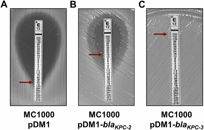
A Antibiotic gradient strip on a lawn of E. coli MC1000 pDM1 from biological repeat #1, showing an MIC value of 0.25 μg/mL (red arrow). B Antibiotic gradient strip on a lawn of E. coli MC1000 pDM1-bla_KPC-2 from biological repeat #1 showing an MIC value of 16 μg/mL (red arrow), determined by considering the single colonies framing the inhibition zone. C Antibiotic gradient strip on a lawn of E. coli MC1000 pDM1-bla_KPC-3 from biological repeat #1 showing no inhibition zone. The MIC value in this case is recorded as >256 μg/mL (red arrow).

Full size image

Using this method, the control strain E. coli ATCC 25922 exhibits MIC values of 0.25 μg/mL (Table 4, Fig. 3A), which are within the acceptable quality control range^7,18. The empty-vector control strain, E. coli MC1000 pDM1, has the same low ceftazidime MIC value. By contrast, two β-lactamase-expressing strains, E. coli MC1000 pDM1-bla_KPC-2 and E. coli MC1000 pDM1-bla_KPC-3, show high MIC values (Table 4, Fig. 3A) and would be labeled as resistant according to the EUCAST (the ceftazidime clinical breakpoint is at MIC > 4 μg/mL⁹) and CLSI (the ceftazidime clinical breakpoint is at MIC > = 16 μg/mL²⁰) breakpoints.

Finally, when using gradient strips, the clarity of the results may be affected by the bacterial strain, the type of the antibiotic tested (bacteriostatic/bactericidal), the resistance mechanism encoded by the tested organism, or by user errors²¹. Some of the common challenges confounding the identification of MIC values using antibiotic gradient strips are summarized in Table 5, and follow-up actions are provided. For additional guidance and information, the antibiotic gradient strip manufacturer’s instructions should be consulted.

MIC values determined using the broth microdilution method (Protocols 2a/2b/2c)

Following the last incubation step, the positive growth-control wells (Fig. 2, ‘+’) should exhibit solid bacterial growth, while the negative growth-control wells (Fig. 2, ‘–’) should only contain clear broth. Lack of growth in the positive growth-control wells or growth in the negative growth-control wells invalidates the MIC assay, which must be repeated. The MIC value is read as the lowest antibiotic concentration where no growth is visibly observed (Fig. 2E, growth in red, no growth in light blue, MIC well denoted by a star).

Assessment of ceftazidime MICs based on visible growth using this method shows comparable values (Fig. 3; compare panels A and B) to those recorded using the antibiotic gradient strip for all tested strains. In general, a twofold difference in MIC values is not considered significant. As such, the ceftazidime MIC values for E. coli MC1000 pDM1-bla_KPC-3 (12–24 μg/mL using gradient strips and 16–32 μg/mL using broth microdilution) are in essential aggreement.

Assessment of colistin MICs based on visible growth using broth microdilution shows an MIC value of 1 μg/mL for the E. coli ATCC 25922 quality control strain (Table 4, Fig. 3C), which is within the acceptable quality control range^7,18. The empty-vector control strain has the same low colistin MIC value (Table 4, Fig. 3C). A strain harboring a mobile colistin resistance gene on a plasmid, (E. coli W3110 pDM1-mcr-1) and a strain that is colistin-resistant through a chromosomal mutation (E. coli WD101²²), show MIC values of 4 and 16 μg/mL, respectively (Table 4, Fig. 3). Both strains would be considered resistant according to EUCAST, since the clinical breakpoint for colistin is at MIC > 2 μg/mL⁹ and CLSI, whereby the colistin clinical breakpoint is defined as MIC ≧ 4 μg/mL²⁰.

Determination of MIC values using broth microdilution may be affected by trailing growth or the presence of wells with no visible growth in-between wells with visible bacterial growth. These challenges likely arise because of specific bacterial strain effects, antibiotic effects, and/or user errors. The use of a plate reader to help assess the turbidity of MIC wells may be implemented in these cases. However, care should be taken to ensure that OD600 values, denoted as the lowest limit for bacterial growth, are visible to the naked eye. The assignment of bacterial growth for wells where the OD600 values are higher than the negative growth-control well but cannot be clearly distinguished by the naked eye is incorrect according to current guidelines. Some of the most common challenges confounding the identification of MIC values using the broth microdilution method are summarized in Table 6, and follow-up actions are provided. For additional information, we refer the readers to the EUCAST reading guide for broth microdilution⁶ or the CLSI MIC troubleshooting guide⁷, which offer further guidance on a wider variety of observed phenotypes (see also Supplemental File 1).

Finally, it should be noted that MIC values are known to exhibit one to twofold variation between different laboratories, users, and MIC value determination techniques. It is generally accepted that this variation is not significant and values that fall within this range are broadly considered to be in ‘essential agreement’²³. Nonetheless, it should be noted that a twofold differences at high MIC values can denote significant changes in survival under antibiotic pressure and should, thus, be treated with caution¹¹. Caution should also be used when considering the MICs of agents where the antimicrobial range may be functionally compressed. For example, a large fraction of colistin-resistant isolates that harbor mobile colistin resistance genes exhibits colistin MIC values of 4-8 μg/mL. These MIC values are comparable to the clinical breakpoint values for colistin; the E. coli resistance breakpoint is >2 μg/mL and ≧4 μg/mL by EUCAST⁹ and by CLSI²⁰, respectively. In this case, disregarding one or twofold variations in the measured colistin MICs, may lead to erroneous characterization of isolates as colistin susceptible or resistant. To aid in the determination of the commonly observed MIC ranges for different bacterial species, we refer the readers to the EUCAST MIC distribution database²⁴.

MIC assays are an ISO standardized (ISO 20776-1:2019) approach for antimicrobial susceptibility testing and are used both by research and diagnostic laboratories. The protocols described herein are representative of the EUCAST recommendations for testing of non-fastidious organisms, however standardized methods from the CLSI are also widely used for antimicrobial testing.

Irrespective of the health standard body used to assess antimicrobial susceptibility, standardized MIC assays must be carried out without any modifications to the core components of each specific method, while several quality control steps must be taken for the data to be reproducible across users and laboratories. Key components of MIC assays that should not be adapted or omitted are:

i) the use of pure cultures, validated by sub-culture on non-selective agar concurrently with the MIC assay

ii) the use of the correct bacterial inoculum of 5 × 10⁵ CFU/mL^7,9,18

iii) the use of specific growth conditions

iv) the inclusion of positive and negative controls for bacterial growth (broth microdilution only)

v) the determination of MIC values for quality control strains¹⁸

It should be noted that while the inoculum amounts are strictly defined (CFU/mL should remain at 5 × 10⁵), there are several methods that can be used for its preparation²⁵. This may be of particular interest for research endeavors where changes in growth conditions prior to the MIC assay may be required or could provide valuable additional information on the studied system. In cases where more expansive changes to the protocol are required, for example during the study of new organisms or for assessment of specific growth conditions, these modifications must be clearly described, and the assay should be denoted as an adapted MIC experiment. Where possible, the values obtained through adapted MIC experiments should be validated using quality control strains and compared to results recorded using the standardized reference methods.

Finally, although MIC assays are commonly associated with antibiotic compounds, similar experiments can be used to study the effects of many other chemical agents on bacterial growth. As such, MIC methods described here can be leveraged and appropriately adapted for the design of assays to assess bacterial growth under diverse chemical pressures.