Water and wastewater infrastructure inequity in unincorporated communities

Introduction
Underinvestment and uneven access to water and wastewater infrastructure are shaped by local governance. The U.S. is one of the only countries in the world with large populations living outside of city bounds, in unincorporated areas. Most countries do not have unincorporated areas or such locations are remote and uninhabited. Yet, in the U.S., unincorporated areas can be located in the midst of metropolitan regions. Communities on the margins of incorporated places have less political representation, tend to be inhabited by marginalized populations, and can lack piped water and sewer services1,2,3,4.
Nearly 37% of the U.S. population lives in unincorporated areas5,6, not all of which are densely settled communities. Despite their prevalence, unincorporated communities are overlooked by the empirical literature within water resources, geography, and urban planning7, and the broader environmental justice literature8. It is unknown how many unincorporated communities exist, how they are distributed, and their level of access to water and wastewater services. Research in the U.S. is limited by inconsistent recognition by the Census Bureau, which identifies a subset of unincorporated communities, yet leaves an unknown number invisible9. At the same time, comprehensive delineations of water and wastewater service areas are not nationally available.
Communities not served by centralized infrastructure rely primarily on septic systems and domestic wells; some U.S. households lack wastewater treatment and/or piped drinking water10,11. Nearly 25% of U.S. households are not connected to centralized sewer12,13,14 and 13% of the U.S. population are not served by public water systems15. Septic systems fail at alarming rates16,17,18, due to a lack of upkeep16,19 or adverse soil and weather conditions. This contributes to environmental impairment; higher septic tank density in neighborhoods is associated with a greater risk of diarrheal illness20. Domestic wells are not regulated under the Safe Drinking Water Act; while waterborne disease outbreaks have declined in public water systems since the 1970s, detected outbreaks for domestic wells have risen21,22.
In the absence of a local municipal government, unincorporated areas are governed by county authorities, which are less powerful23 and have fewer revenue-generating options. To attract taxable business activities, counties might allow undesirable land uses24,25. Exclusion from local government can occur through municipal underbounding, which is selective boundary expansion based on neighborhood income or racial composition. This practice can cause cities to expand around or away from lower-income communities of color4,24,26,27,28,29,30. Evidence of underbounding extends across the country1,24,28,31,32,33. Municipal governments may justify incorporation decisions based on the financial burdens of annexing lower-income communities34. A majority of unincorporated settlements in the U.S. are predominantly Latino or African American24. On the edges of incorporated areas, such communities lack municipal voting rights and can be excluded from municipal services1,4,8,24,33,35,36,37; immigration status can worsen this issue38.
While other utility services are provided regionally, water and sewer services tend to be localized. Over 16,000 publicly-owned wastewater treatment works and 50,000 community water systems exist nationwide, compared to only 1200 natural gas and 3000 electricity providers29. The vast majority of the 471,000 U.S. households lacking piped water are in urbanized areas, near a public system30. This raises questions regarding the extent to which incorporation status can explain gaps in coverage. The scale of inadequate wastewater infrastructure in unincorporated communities is anticipated to become worse, as new housing developments expand into these areas and an increasing portion of new homes rely on septic systems39,40.
Distinct features of unincorporated communities could produce inadequate infrastructure access. Such communities are reliant on counties; compared to municipalities, counties have less ability to provide utility services and political representation24. At the same time, unincorporated communities face diluted voting power. While all county residents can vote for county commissioners, only unincorporated residents are entirely dependent on county-level decision-making, and so can be underrepresented on issues that disproportionately affect them41,42.
Selective annexation can create operational inefficiencies due to noncontiguous service territories that are inefficient and costly to serve. Unincorporated communities cannot initiate annexation and are subject to the decisions of municipal and county governments24,43. Self-incorporation is typically infeasible since communities in close proximity to an existing municipality often do not meet the legal criteria for incorporation, which varies by state (Supplementary Table 1).
Unincorporated communities can face limited financial control due to extraterritorial planning jurisdiction. Municipalities in many states are granted zoning and other land use planning powers a certain distance beyond city boundaries44. This can limit the ability of counties to improve their tax base, particularly through property tax revenues that commonly fund water and wastewater services. While many municipalities provide drinking water to areas beyond city limits; fewer provide sewer service45. Federal funding for water and wastewater can be difficult for unincorporated communities to access. Often, funding supports municipal-owned, centralized systems46,47. Individual homeowners are typically ineligible48 and community-based organizations rarely receive Clean Water State Revolving Fund financing13. Unincorporated communities face barriers since federal applications require a responsible management entity to establish a billing system and pay upfront installation costs49.
Few studies have addressed municipal incorporation as a structural determinant that can produce inequities in infrastructure access. Past studies have found that low-income and minoritized populations are less likely to be served by public water systems50,51,52 and sewer systems45. If connected to public water, such communities can be more likely to face impaired water quality53,54. Without examining jurisdictional differences, past efforts can overlook underlying drivers of and remedies for infrastructure inequities. Past studies tend to feature individual cases of unincorporated communities28,55 or multiple communities within one state31,45,51,56,57. No previous research has quantified the influence of incorporation status on infrastructure access at a regional scale or across multiple states.
This study examines municipal incorporation as a structural determinant of infrastructure inequities. Negative binomial models assess how incorporation status shapes access to centralized infrastructure. Our study sample comprises 31,383 block groups located in nine states, representing over 25% of the national population—Connecticut, Florida Kentucky, Mississippi, New Jersey, North Carolina, Rhode Island, Texas, and West Virginia (Fig. 1). Across these nine states, we estimate that over 10 million people live in unincorporated communities. If these unincorporated communities were a state, they would have more residents than 41 states.

This map depicts incorporated and unincorporated communities included in our study. Incorporated communities are located within city boundaries. Three northeastern states (Connecticut, New Jersey, and Rhode Island) only contain incorporated communities; unincorporated areas do not exist within these states. See the “Methods” section for a full data description.
To render all unincorporated communities visible, we develop an approach to comprehensively identify and categorize unincorporated communities, by combining spatial datasets on building footprints, land use, and municipal boundaries. We develop a spatial dataset for centralized sewer and water infrastructure across the nine-state study region. Our study objectives are to: (i) identify the prevalence and distribution of unincorporated communities, (ii) examine the association between incorporation status and infrastructure coverage, and (iii) determine how poverty rates are associated with coverage and whether the effect of poverty differs across incorporation status.
Overall, this study provides insight into disparate water and wastewater access. Improved understanding of disparities across jurisdictions can target assistance and policies to extend critical infrastructure to underserved communities.
Results
Types of unincorporated communities
Overall, across all nine states, 47% of the total community land area is unincorporated. We define community land as settlements that surpass the equivalent of 250 parcels per square mile, a threshold used in previous literature56. Our study focuses on block groups that meet this housing density threshold. In four states, over half of community land is unincorporated communities in Florida, Kentucky, North Carolina, and West Virginia (Fig. 2a). In terms of population, across the nine study states, we find that over 10 million people live in unincorporated communities, representing 21% of the population of community land. The portion of the population residing in unincorporated communities varies widely across states, from 0% in Northeast states to 42% in Florida. Large variation also exists across states in the typologies of unincorporated communities (Fig. 2b).
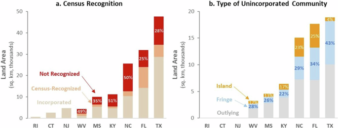
a Depicts the land area of incorporated and unincorporated communities, in thousands of sq km. Two categories of unincorporated communities are presented—those that are recognized by the Census Bureau (‘Census-Recognized’) and those not recognized (‘Not Recognized’). Labels containing percentage values represent the percentage of community land area in a given state that is unincorporated and not recognized by the Census Bureau. Land area is restricted to ‘communities’, which are defined based on housing density greater than 250 parcels per square mile, a threshold used in previous literature56. b Presents the land area of three types of unincorporated communities, defined based on based on placement relative to incorporated places. Islands are at least partially surrounded by city boundaries. Fringes are all other unincorporated communities within 1.6 km of an incorporated place boundary. Outlying communities are located beyond 1.6 km from city boundaries. See the “Methods” section for a full data description. Labels containing percentage values represent the percentage of unincorporated community land area in a given state that is categorized as Island communities (shown in white text) and Fringe communities (shown in blue text).
The importance of identifying unincorporated communities beyond those recognized by the Census Bureau is illustrated by Fig. 2a. The Census Bureau recognizes well-known unincorporated communities as census designated places (CDPs), which are concentrations of populations with names that are distinct and locally recognized (see Supplementary Information). Our approach using building footprints to identify additional communities not recognized by the Census Bureau captures 69% of the land area of unincorporated communities across the nine states. Many unincorporated communities are not recognized by the Census Bureau. Across states, there is considerable variation across states in terms of the portion of unincorporated communities identified through our approach—ranging from 45% (for Florida) to 88% (for Kentucky). Variations across states reflect differences in incorporation laws, recent population growth, and preferences about place identification. Identifying unincorporated communities beyond those recognized by the Census Bureau is relevant in all study states that have unincorporated areas.
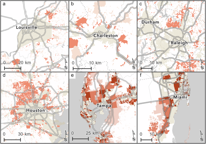
Metropolitan area examples in Fig. 3 illustrate differences in Census recognition. Relatively few unrecognized unincorporated communities exist in Florida metro areas (Fig. 3e, f) and Charleston, WV (Fig. 3b). In addition, although Kentucky overall has a high prevalence of unrecognized communities, the Louisville metropolitan area is an exception due to city-county government consolidation (Fig. 3a). Large tracts of unincorporated areas are not Census-recognized in northwest Houston (Fig. 3d) and in Raleigh–Durham area of North Carolina (Fig. 3c); both are among the fastest-growing major metropolitan areas in the country58. For example, metropolitan areas were selected based on population and distribution of unincorporated communities. In some counties, unincorporated populations surpass one million—in Harris County, TX (1.3 million people) and Miami-Dade County, FL (1.0 million). If these unincorporated populations were cities, they would be the 9th and 10th largest nationally. Other substantial unincorporated populations are located in Hillsborough County, FL which contains Tampa (0.8 million people), and Wake County, NC which contains Raleigh (>85,000 people).

Within the six metropolitan areas above, we depict the land area of communities recognized by the Census Bureau (shown in green) and the land area of unincorporated communities not recognized by the Census Bureau (shown in purple). Recognized communities include both incorporated and unincorporated areas, which are identified as CDPs by the Census Bureau. A full description of CDPs is provided in the “Methods” section. Metropolitan areas depicted are Louisville, KY (a), Charleston, WV (b), Raleigh, NC (c), Houston, TX (d), Tampa, FL (e), and Miami, FL (f).
We classify unincorporated communities based on placement relative to incorporated places. Unincorporated communities are defined as settlements outside of incorporated areas that surpass the equivalent of 250 parcels per square mile. Three categories of unincorporated communities are developed—Island, Fringe, and Outlying. Each type faces different circumstances due to proximity to municipal services and the influence of municipal powers such as annexation and extraterritorial jurisdiction59.
Island and Fringe communities are within close proximity to city limits. Islands are partially or fully surrounded by city limits—we specify this as an unincorporated community with at least one-third of its perimeter within 480 m of an incorporated place boundary. Fringes are all other unincorporated communities within 1.6 km (1 mile) of an incorporated place boundary, which is considered an approximation for the extent of municipal extraterritorial jurisdiction56,60. Outlying communities are located far from municipal boundaries; further than 1.6 km.
By classification of unincorporated communities, Islands and Fringes are more prevalent in states with major population centers, while outlying communities are prevalent in states with less population density (e.g., Kentucky, Mississippi, West Virginia). About one-quarter of the total community land area is within Islands or Fringes. Island and Fringe communities are likely to be within municipal extraterritorial jurisdiction. In some states, over 30% of community land area is likely within extraterritorial jurisdiction—Florida, North Carolina, and West Virginia. Islands are especially prevalent in Florida and North Carolina (Fig. 2b). Fringes are also common in these two states, in addition to Texas and West Virginia. Metropolitan area examples in Fig. 4 further highlight the ubiquity of Islands and Fringes in Florida (Fig. 4e, f), The Raleigh–Durham area of North Carolina (Fig. 4c), and northwest Houston (Fig. 4d). Outlying and Fringe communities are present in Charleston, WV (Fig. 4b) and Louisville, KY (Fig. 4a). Although, due to city-county consolidation, Louisville has comparatively smaller tracts of unincorporated area.
Within the six metropolitan areas above, we depict the land areas of several incorporation statuses—incorporated (depicted in beige) and three types of unincorporated—Islands (darkest red), Fringes (medium red), Outlying (lightest red). Incorporated communities are located within city boundaries. Unincorporated communities are defined based on based on placement relative to incorporated places. Islands are at least partially surrounded by city boundaries. Fringes are all other unincorporated communities within 1.6 km of an incorporated place boundary. Outlying communities are located beyond 1.6 km from city boundaries. See the “Methods” section for a full data description. Metropolitan areas depicted are Louisville, KY (a), Charleston, WV (b), Raleigh, NC (c), Houston, TX (d), Tampa, FL (e), and Miami, FL (f).
Municipal annexation policy might partially explain widespread Islands in Florida and North Carolina. In particular, North Carolina has a well-known history of municipal underbounding; it was one of the few states allowing involuntary annexation, where municipalities can add new territories without the consent of unincorporated residents61. Municipalities would be incentivized to involuntarily annex areas with higher-value properties. While involuntary annexation was constrained in 2011 (Supplementary Table 1), municipal boundaries remain shaped by past decisions. Florida, in contrast, has state-level contiguity requirements for annexation, yet municipal annexation ordinances persist even in cases where they create islands2. In addition, a state-level requirement to provide water and sewer services prior to annexation might deter the incorporation of some Islands, despite substantial state investment to bring infrastructure up to municipal code standards in unincorporated areas of urbanized counties. Also, Florida has had a history of developer bankruptcies, which have deprived major subdivisions of promised infrastructure62.
Fringes in Texas might be explained by the ability of municipalities to involuntarily annex small-population, unincorporated Islands (Supplementary Table 1). This could result in a high prevalence of fringe communities, while reducing the presence of Islands. In addition, Texas has over 2000 documented colonias63, which are a sub-type of unincorporated communities and tend to be located in unincorporated Fringes or Outlying locations. Meanwhile, Fringes in West Virginia could be due to the geographic distribution of settlements—small, isolated municipalities surrounded by unincorporated land44.
Patterns of sewer service and incorporation status also differ across states, as illustrated in Fig. 5. The degree to which service areas extend to unincorporated areas can be influenced by annexation policy, required services for incorporation, and extraterritorial planning power. Required services for annexation vary across states (Supplementary Table 1); among our study states, only Florida, Texas, and Louisville require water and sewer services. Notably, North Carolina does not condition annexation on any public services. Louisville has some incorporated areas and fringes not served by centralized sewer (Fig. 5a); widespread coverage in the metro area might be due to the consolidated city-county government; formed in 2003, it is the most recent of only 34 city-county consolidations nationwide. In contrast, extensive fringe communities in the Raleigh–Durham area are not connected to sewer service (Fig. 5c); this might be partly explained by municipal underbounding and pre-2011 extraterritorial planning power. A different distribution of services is illustrated by Charleston, WV (Fig. 5b); here, outlying communities are not served, while portions of fringes are; population density might play a larger role in shaping access in this example.
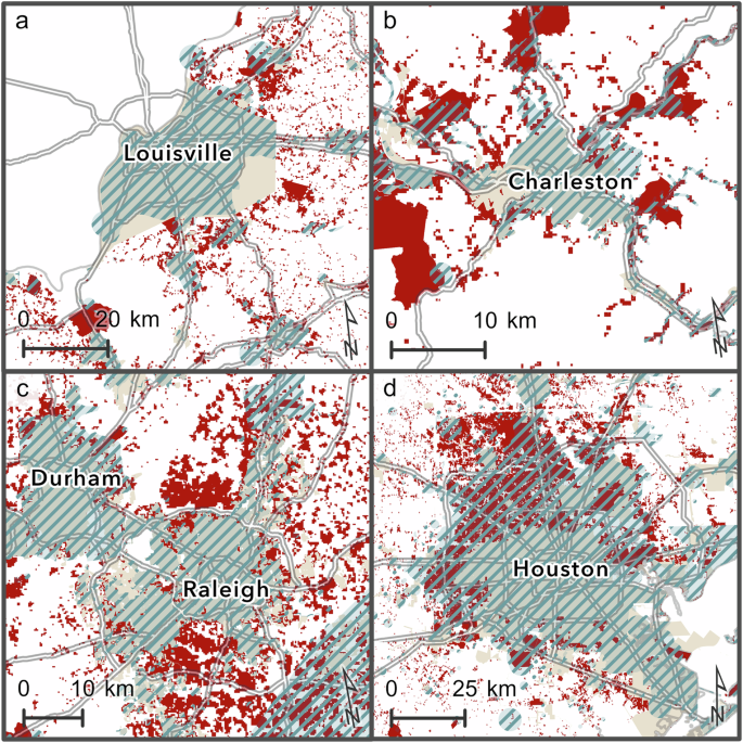
Within the four metropolitan areas above, we depict incorporation status (incorporated and unincorporated), as well as areas served by sewer infrastructure. Incorporated communities are located within city boundaries (depicted in beige), while unincorporated communities are not a part of a municipal government (depicted in red). Sewer service areas are developed from multiple data sources (sewered areas are depicted with blue crosshatch). See the “Methods” section for a full data description. Metropolitan areas depicted are Louisville, KY (a), Charleston, WV (b), Raleigh, NC (c), and Houston, TX (d).
Summary statistics
Our unit of analysis is the Census block group, since these are the smallest geographic areas for which the Census Bureau provides sample data. Block groups are statistical sampling units defined by the Census Bureau; they are between a Census block and a Census tract in terms of geographic level. Boundaries of block groups should follow visible or non-visible features, such as roads, rivers, and administrative boundaries. In our study sample, block groups have an average population of 1538 (ranging from 10 to 28,537 people) and a land area of 2.37 sq km (ranging from nearly zero to 7760 sq km) (Supplementary Table 2).
In our sample, centralized infrastructure coverage is extensive overall. While the vast majority of block groups have universal coverage, large variations in sewer coverage exist within unincorporated communities. Gaps in sewer coverage are much greater than centralized water service. On average, 14% of block group land area is unsewered, compared to 5.6% of land area not served by centralized water (Supplementary Table 2); in addition, the standard deviation for the portion of area unsewered is substantially greater.
Incorporated communities represent the majority of the study sample – 83% of block group observations (Supplementary Table 2). This is expected since block groups are statistical sampling units defined by the Census Bureau. Typically, block groups contain several thousand people, which results in many small area block groups in urban areas, and few block groups with larger areas in less dense locations. Islands and Fringes represent about 6% and 8% of block group observations, respectively; while Outlying block groups have the fewest observations (n = 845, 2.7% of the study sample). Population density differs across incorporation status. Unincorporated communities have substantially less population density on average (Supplementary Table 3). Fringes and Outlying communities tend to have the sparsest density, which is mostly due to larger block group land area. In particular, Outlying communities have the largest variation in land area.
Across incorporation status, large variations in sewer coverage exist, which are not as pronounced for centralized water (Supplementary Tables 3 and 4). Islands have the largest gap between centralized water and sewer service. Islands have the highest portion of land area unsewered (median = 15%), followed by Fringes (3.7%) and Outlying communities (3.1%) (Fig. 6a and Supplementary Table 4). For incorporated block groups, the median percent land area unsewered is nearly zero; about 48% of incorporated block groups have no area that is unserved by sewer. For water, the median percent land area unserved is near-zero for all community types (Fig. 6b). Above the median, Fringe, and Outlying communities tend to have the largest portion of land area not served by centralized water.
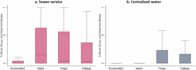
We present box plots of the percentage of land area not served, for sewer (a) and drinking water (b) infrastructure. Incorporated communities are located within city boundaries. Unincorporated communities are defined based on based on placement relative to incorporated places. Islands are at least partially surrounded by city boundaries. Fringes are all other unincorporated communities within 1.6 km of an incorporated place boundary. Outlying communities are located beyond 1.6 km from city boundaries. See the “Methods” section for a full data description.
Poverty rates and sewer coverage are related within unincorporated block groups (Fig. 7). Islands and Outlying communities within the highest poverty tercile (≥20.5% of households below the poverty line in block group) face the largest portion of unsewered area, while Fringes and Outlying in the highest poverty tercile are the most underserved by centralized water. Islands and Outlying block groups with the highest tercile of poverty tend to have higher portions of land area not served by sewer infrastructure. Yet, among incorporated block groups, the variation in coverage declines with higher poverty. Water coverage, in contrast, is consistently high across incorporation status. Highest tercile poverty Fringes and Outlying communities tend to have the largest portion of land area not served by centralized water. Few communities that are Islands or Incorporated have a substantial portion of land area not served by centralized water. Islands and Outlying block groups in the highest tercile of poverty have median areas unsewered that are an order of magnitude larger (19.0% and 11.8%, respectively), compared to Fringe (4.5%) and Incorporated communities (0%). Poverty rates vary across incorporation status. Unincorporated communities tend to have lower poverty rates, on average, especially within Fringe and Outlying block groups (Supplementary Tables 3 and 4). Islands have the highest average poverty rate among unincorporated communities.
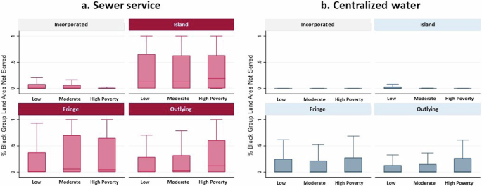
For sewer (a) and drinking water (b) infrastructure, we present box plots of the percentage of land area not served. Poverty terciles are defined as low (<7.39% households below the poverty line in the block group), moderate (7.39–20.5%), and high (≥20.5%). Incorporated communities are located within city boundaries. Unincorporated communities are defined based on based on placement relative to incorporated places. See the “Methods” section for a full data description.
Regression results
Regression results indicate that unincorporated communities face a greater relative risk of land area unserved by sewer and water infrastructure. We also find that the effect of high poverty on unserved areas is greater for unincorporated communities, both for sewer and centralized water. Among high-poverty block groups, unincorporated status is associated with 3.54 times greater unsewered area and 17.8 times more area unserved by centralized water (Supplementary Table 5). These estimated incidence rate ratios (IRRs) are several times greater for high-poverty blocks compared to those without high poverty levels. Among block groups without high poverty, unincorporated communities compared to incorporated are expected to have 1.48 times greater unsewered area (Supplementary Table 5), while holding constant population density and other factors.
Model specifications with random effects have a better fit, based on the Akaike information criterion. When considering county and state random effects, the percent rural population is not significantly associated with sewer or water coverage (Supplementary Tables 5 and 6).
Our main results consider the three types of unincorporated communities and their interactions with high poverty rates. A block group is designated as having high poverty if 20% or more of households are below Federal poverty line64. This allows us to examine whether the effect of high poverty on the relative risk of unserved land area differs between incorporated and unincorporated communities. For unsewered areas, the effect of being unincorporated is much greater for high-poverty block groups (Fig. 8 and Supplementary Table 6). Outlying and Island communities especially have greater IRR estimates for high-poverty block groups, which are several times higher than IRRs estimated for block groups without high poverty. For high-poverty block groups, both Outlying and Island communities are associated with an increase in unsewered areas by a factor of over 4.0. In contrast, Outlying communities without high poverty are associated with less unsewered areas (IRR = 0.91). Fringe communities also have greater estimated IRRs for high-poverty block groups, yet the difference between high and low-poverty block groups is smaller compared to Outlying (IRR is 4.6 times greater for high-poverty) and Island communities (2.4 times greater).
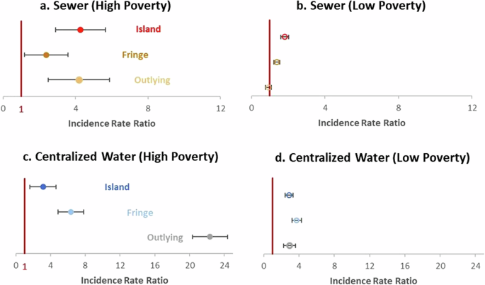
For sewer and drinking water infrastructure, we present regression results from our preferred model specification. Estimated IRRs for sewer coverage are presented for high-poverty block groups (a) and those with low poverty, <20% of households below the Federal poverty line (b). For centralized water, estimated IRRs are presented in (c, d). The referent category for incorporation status is incorporated; thus, all comparisons are made to incorporated block groups. Furthermore, all estimates are conditional on the county and state; our model includes random effects at the county and state levels. See “Methods” for a description of regression models and data. Full regression result tables are provided in Supplementary Table 6, models 6 and 8.
We find that estimated IRRs for indicators of three types of unincorporated communities and interactions with high poverty rates differ across water and sewer infrastructure. Outlying and Fringe communities have much larger IRR estimates for areas unserved by centralized water in high-poverty block groups (Fig. 8 and Supplementary Table 6). The effect of high poverty on centralized water coverage is greater than for sewer service, particularly for Outlying and Fringe communities. In contrast, for Island communities, IRR estimates for centralized water do not differ considerably by poverty level.
In models that do not include a high poverty interaction, Outlying communities have the largest magnitude estimate for area unserved by centralized water (IRR = 5.53) (Supplementary Table 6). In contrast, for sewer coverage, Island communities have the largest IRR estimate for unsewered area (IRR = 2.47) (Supplementary Table 6).
Discussion
Access to basic sanitation is recognized as a fundamental human right by the UN Sustainable Development Goals. In unincorporated areas in the United States, this right might not be realized. We find that incorporation status shapes differential access to water and wastewater infrastructure. Three key findings emerge from this study. First, we find evidence that unincorporated communities are underserved, relative to incorporated communities. Lack of sewer access is more prevalent than in areas not served by centralized water. Nearly 30% of land area in unincorporated communities is not sewered, compared to 11% in incorporated communities, on average. Higher costs of sewer service, relative to centralized water, may partly explain this gap65. Sewer coverage rates are significantly lower for unincorporated communities in close proximity to municipal boundaries, such as Islands and Fringes. In contrast, for centralized water, Outlying communities are most strongly associated with lower coverage. Local jurisdiction creates bright lines that divide served and underserved communities, particularly for sewer infrastructure. Where unincorporated communities begin, sewer lines tend to wane. Island and Fringe communities might be especially prone to being underserved by sewer infrastructure due to municipal underbounding, extraterritorial jurisdiction, and state laws that restrict new incorporations in proximity to existing municipalities.
Second, coverage is associated with the poverty rate. High poverty Islands and Outlying communities face the largest portion of unsewered areas, while high poverty Fringes and Outlying are the most underserved by centralized water. Regression results indicate that the association between high poverty and unsewered areas is greater for unincorporated communities than incorporated ones. This association holds across all three types of unincorporated communities. In contrast, for centralized water, Islands do not have a significantly greater effect of high poverty than incorporated communities. High poverty rates appear to influence the ability of a community to attract amenities such as centralized infrastructure and may have a bearing on its relative power within county government. Unincorporated communities differ drastically by income, ranging from underserved, lower-income neighborhoods to higher-income gated communities with privately-provided services2. Higher-income communities have greater choice over which centralized services to develop or purchase24; for example, by forming special assessment districts or organizing to purchase municipal services. In addition, higher-income communities outside of city bounds might fill the local governance gap with homeowner associations that provide utility services. For example, Outlying communities without high poverty rates are not found to be significantly associated with unsewered areas.
Third, differences in results across water and sewer infrastructure have implications for prioritization. One difference is that unsewered areas tend to be more extensive than areas not served by centralized water. Unincorporated communities face a considerably greater lack of sewer coverage. This suggests that the extension of sewer services is a more widespread issue. Another difference is that priorities for targeting communities for water and sewer extensions might differ. For sewer assistance, it could be justifiable to prioritize high-poverty unincorporated communities, especially Islands and Fringes. Islands have the largest magnitude incidence rate ratio for unsewered areas. Yet, for water service extension, high poverty Outlying and Fringe communities would be top priorities. Outlying communities have a particularly strong association with areas unserved by centralized water. These findings suggest that the current emphasis on rural, unincorporated communities for Federal drinking water assistance might be justified. However, a different prioritization is likely appropriate for wastewater assistance.
Policy reforms at the state and Federal levels could address spatial inequities. Water and sewer planning, unlike other hard infrastructure, is regaled to the most local levels, typically county and municipal governments. Local levels can lack the capacity for comprehensive and sustained planning. Unincorporated communities are often without an adequate voice. This status quo is untenable with over $470 billion in upgrades needed for aging water infrastructure and over $270 billion for wastewater treatment facilities over the next 20 years66, let alone communities not yet served. Planning responsibility and funding are overwhelmingly borne by local governments and service providers; Federal funding only represents 4% of annual spending on water and wastewater utility infrastructure67.
We suggest four policy reforms: (i) strengthening regional water planning and participatory governance, (ii) recognizing underserved, unincorporated communities, (iii) enabling the use of modular, decentralized infrastructure, and (iv) enhancing the role of county governments in annexation and infrastructure decisions.
First, regionalizing water planning could address underserved and unincorporated communities by shifting away from hyper-local water systems. State or Federal legislation could facilitate this shift, broadening stakeholder involvement and bridging local jurisdictions. Existing regional councils, established by the Housing Act of 1954 and consisting of multiple local governments, could be pivotal in this process. These councils assist with planning, funding applications, and project management. With over 500 councils serving more than 35,000 local governments, they are well-positioned to support regional water planning. In contrast to water, transportation planning at regional levels is facilitated by dedicated institutions—Metropolitan Planning Organizations, which bring together municipal and county officials as well as state agencies that manage transportation. A similar model could be used for water by forming regional water organizations within existing regional councils, allowing residents of unincorporated areas to hold council seats, and allowing regional councils to administer state-revolving funds on behalf of unincorporated communities. In addition, state legislation could create advisory councils to allow unincorporated communities to voice concerns before county supervisors, such as in California.
Second, recognizing unincorporated Island and Fringe communities is a prerequisite for reconciling infrastructure inequities. Many of these communities lack state or Federal recognition, which limits access to funding and other support. Colonias gained Federal recognition through the National Affordable Housing Act of 1990, enabling access to support from the USDA, HUD, and EPA. At the state level, California requires boundary commissions to identify low-income unincorporated communities within city spheres of influence; city general plans must assess the infrastructure needs of these communities. In addition, at least 23 states have some form of law discouraging the creation of Islands or facilitating their annexation. However, narrow definitions of Islands in many states often exclude communities that are functionally islands yet not entirely surrounded by city limits, such as those sharing boundaries with waterbodies and state-owned land. Adopting revised definitions of islands, such as the one developed for this study, could improve the effectiveness of policies aimed at supporting such communities.
Third, modular, decentralized infrastructure offers a flexible solution for noncontiguous service areas. Such systems offer a paradigm shift, away from the stark choice between large-scale centralized sewer or single-household septic. These connect multiple households to a shared, liquids-only collection and treatment unit, with each household retaining an underground tank for solids. By pooling costs across several households, this approach facilitates affordable bills and financially sustainable operations68. Such decentralized system typology can address the geographies of underserved unincorporated communities, which feature urban Islands and housing clusters in rural areas. Modular, decentralized systems could serve as an interim measure before centralized services are extended or as a long-term solution.
Fourth, enhancing the role of counties in annexation and regional infrastructure investment decisions could grant greater political power to unincorporated communities. This addresses the legacy of exclusionary planning and zoning. In most states, only municipal residents and those living in areas proposed for annexation have a voice. Yet, county governments and residents of unincorporated areas not slated for annexation are affected politically and financially. State laws could grant counties review authority of proposed annexations and require municipalities to assess the fiscal and service effects of annexation on the county. Additionally, we suggest establishing a third-party entity for annexation decisions to improve the representation of counties, either through municipal courts (a weaker option) or state-level boundary commissions (a stronger option). Boundary commissions provide equal representation of county and municipal governments in boundary change decisions; these commissions have only been established in a few states, such as California. As an extreme option, consolidated city-county governments address unincorporated areas by fully incorporating a metropolitan area under one government.
States could empower county governments to petition for municipal annexation or utility service extensions on behalf of unincorporated communities, shifting costs away from residents. Currently, only Arizona permits counties to initiate annexation of small unincorporated Islands. Petitions could especially be justified for public health concerns or involuntary annexation. For public health, state-revolving funds could be prioritized for projects that address underserved communities via service extension or annexation. States would need to also address aspects of municipal and county planning that can limit service extension. For example, in Washington, the Growth Management Act restricts extensions beyond urban growth boundaries. Residents should generally retain the choice to connect (or not) to centralized infrastructure, although mandatory connections and/or subsidized services may be justified in cases of environmental impairment in downstream communities. Some states, such as Florida, Oregon, and West Virginia, allow mandated sewer connections or involuntary annexation for public health reasons.
In the case of involuntary annexation, states could require municipalities to annex lower-income communities before approving the annexation of higher-income areas, similar to inclusionary zoning laws that mandate affordable housing for development entitlements. Such policies could improve infrastructure in urban fringes. Alternatively, unincorporated residents denied annexation might be able to purchase extraterritorial utility services.
Annexation and service extension will not be desirable to all unincorporated communities due to higher service costs and greater regulation34. Without addressing the affordability of utility services, the price of crossing the municipal boundary can be out of reach. Service extensions can be more appealing if upfront infrastructure costs and connection fees are externally funded2. In addition, customers outside of municipal boundaries are often charged considerably higher rates for municipal-provided sewer and water69. Some states, such as North Carolina, have addressed these issues by eliminating connection fees for newly annexed communities and only allowing periodic user fees. Others, such as Georgia and Rhode Island, require that differential rates be based on the cost of service.
Future research would be useful to further examine spatial inequities in water and wastewater infrastructure and identify promising solutions. Difficult questions center on how county and municipal governments should be organized to address service coverage in unincorporated areas. What policies and governance arrangements can address spatial inequities? How should municipalities and counties coordinate planning, especially at jurisdictional boundaries? Which units of government should provide services to unincorporated communities? Possibilities include municipal service extensions as well as modular, decentralized systems managed by county governments or other entities.
Methods
Negative binomial regression
Negative binomial regression models are used to examine the relationship between infrastructure coverage, jurisdiction, and poverty. Our dependent variable is land area not served by centralized infrastructure, over the total block group area. We selected a Negative Binomial Generalized Linear Model (GLM) with random effects at the county level, which is appropriate for count data. Land areas have non-negative integer values. This model was preferred over a Poisson GLM to allow for separate estimates of the mean and the variance of the response variable. The variance in our response variable is larger than the mean, which is referred to as overdispersion. If overdispersion is not accounted for, this can lead to deflated standard errors for coefficients of interest70. Including random effects, at the county level, allows us to account for the correlation among proximate block groups that share more similarities than we are able to account for with observed covariates. In addition, while our response variable includes a large number of zeros (i.e., block groups without unserved areas and thus are fully served), a Vuong test indicates no preference between the zero-inflated model and one without, and we, therefore, select the more parsimonious model.
We estimate the following regression model, where Yij is a negative binomial random variable:
where ({mu }_{{ij}}) is the mean of the land area not served (Yij) in block group i within county j. ({V}_{{ij}}) is a vector of incorporation status indicators, ({X}_{{ij}}) is a vector of other block group characteristics (e.g., high poverty indicator, population density, and percent rural population), ({mathrm{ln}A}_{{ij}}) is an offset term that is the natural log of total block group area (({A}_{{ij}})),(,{u}_{j}) are county-level and state-level errors (random effects), ({varepsilon }_{{ij}}) block group level errors. Since our variable of interest is the proportion of land area unserved in each block group, we include an offset term to account for block groups having different land areas. Block groups are statistical sampling units that are not uniform in land area. In our study sample, the block group land area ranges from 16 sq m to 7760 sq km (Supplementary Table 2). This creates large differences in exposure between block groups—larger block groups have a greater degree of opportunity for counts of unserved areas to accrue. So, we do not model only the land area unserved (Yij); we model the unserved rate, which is the proportion of block group area not served (left(frac{{Y}_{{ij}}}{{A}_{{ij}}}right)).
Random effects in our specification take the form of random intercepts. By including random effects, we aim to account for the correlated nature of our data, and its multilevel structure—block groups are nested within counties and states. It should be noted that coefficient estimates should be interpreted as conditional on the county and state. Block groups within a county and state would not be expected to be independent in terms of infrastructure coverage. Coverage in any given block group would be expected to be correlated with service availability in proximate block groups. In addition, infrastructure coverage within a county and state is related since block groups share unobserved county-level and state-level effects: common county governance, service territory, socioeconomics, environmental characteristics, and other unmeasured factors. County governance factors include annexation policies, strength of government (e.g., authority over land use planning, capacity to provide infrastructure services), and how public officials are elected (e.g., at-large vs by-district elections). Service territories that a county government is responsible for can vary in operational efficiency due to the degree of noncontiguous service area. Environmental factors that could affect infrastructure provision include topography and soil conditions. State factors include different state regulators and permitting agencies for Clean Water Act compliance as well as distribution of state and Federal funds such as Clean Water State Revolving Funds.
Separate models are specified for sewer and centralized water coverage. Factors associated with coverage rates might differ across infrastructure types. We estimate IRR for all models, which are obtained by exponentiating coefficient estimates. For interpreting the interactions between incorporation status and high poverty in a nonlinear model, IRR is an attractive alternative to marginal effects, since it is a multiplicative effect71,72. In specifications that include an interaction term between high poverty and incorporation status, separate IRRs are calculated for unincorporated communities with and without high poverty.
Models control for high poverty, population density, and population distribution within a block group. We examine whether high poverty rates are associated with lower coverage rates and if poverty differentially affects unincorporated communities. Population density is expected to be correlated with the financial and managerial feasibility of centralized infrastructure. Population density will largely determine the cost of provision; yet, where centralized services are financially feasible, incorporation status could influence whether such services are realized. In addition, we control for the percentage of rural population in order to capture how populations are distributed within a block group between rural and urban areas. Summary statistics indicate that while Fringes and Outlying communities have similar population densities, Outlying block groups have nearly double the percentage of the rural population (Supplementary Table 2).
This analysis provides insight into the association between underserved block groups and incorporation status. We note some limitations with the dataset and methods. First, our study sample includes nine states that are located in the eastern half of the continental United States. This should be considered when generalizing the results beyond these nine states. Findings are likely more generalizable to the eastern half of the continental United States, rather than western states. Second, we recognize the potential for our data to have more spatial correlation than is accounted for in our model. A fully spatial model could account for this. However, due to the large amount of data, we decided to implement a model with a simpler correlation structure, since we believe county and state location to be the most relevant variables to account for in an analysis focused on unincorporated communities.
Data overview
We developed a novel dataset of centralized infrastructure coverage and incorporation status at the block group level. Centralized infrastructure coverage is estimated for both drinking water and wastewater using digitized service area boundaries. Incorporation status is identified and categorized based on several datasets, including Census Places73 and Microsoft Building footprints74; details are provided below. We obtained demographic characteristics from the U.S. Census Bureau.
Our study focuses on communities, which are defined as settlements with housing densities greater than 250 parcels per square mile. This threshold is equivalent to an average parcel size of less than 2.56 acres. Only ‘community’ land area is included in the analysis; ‘community’ land areas are 240 m grid cells in a Microsoft building footprint dataset74 that surpasses the equivalent of 250 parcels per square mile. We also remove portions of each cell that meet any of the following criteria: (i) are located within Census blocks with zero population, (ii) have zero land area (i.e., are covered by water), or (iii) are classified by Census Places as parks or military bases.
Block groups are chosen as the unit of analysis since they are the smallest geographic areas for which the Census Bureau provides sample data, such as from the American Community Survey (ACS). We obtain poverty rates from the ACS 5-year estimates for 2008–2012. Block groups are statistical sampling units defined by the Census Bureau; they are between a Census block and a Census tract in terms of geographic level. Each block group consists of several contiguous Census blocks. The Census Bureau aims for block group population to be a minimum of 600 people and a maximum of 3000 people75. Fewer than 600 people is permissible if the county population is also less than 600. Boundaries of block groups should follow visible or non-visible features. Visible features include roads, shorelines, rivers, railroad tracks, or high-tension power lines. Non-visible boundaries include administrative boundaries (e.g., incorporated place and minor civil division) and short line-of-sight road extensions. In urban areas, census block groups are small, approaching the size of a few city blocks. In suburban and rural areas, Census block groups can have large land areas, encompassing thousands of square kilometers.
Identifying incorporated and unincorporated communities
Communities that are incorporated are identified based on the U.S. Census Bureau’s TIGER/Line dataset for the year 201076, as described below. Communities that are unincorporated include both those that are Census Bureau-recognized as well as additional land areas not recognized, as detailed below. For unincorporated communities, we developed a protocol that relies on building footprints74, Census Places73, and several other data sources. Census block groups, our unit of analysis, were categorized as either incorporated or unincorporated. To do so, we intersected Census block group geometry from the year 201077 with our vector datasets of incorporated and unincorporated communities. A block group is designated as incorporated if its incorporated land area is greater than the unincorporated land area. For a block group designated as unincorporated, is further classified as an island, fringe, or outlying block group based on the unincorporated category covering the greatest land area within that block group.
We identified incorporated communities via the Census Bureau Topologically Integrated Geographic Encoding and Referencing (TIGER)/Line dataset for the year 201076; this reports all Census places. We selected Census places with a municipal government based on functional status, class code, and/or inclusion in the Census of Governments. Census places must meet at least one of the following criteria to be designated as municipalities in our study: (1) included in the Census of Governments and has a local government identification number that matches with the US Census TIGER/Line dataset, (2) is functionally a general-purpose government (funcstat = A) and is independent of any county or county subdivision (classfp = C1, C2, C3, C5, C6, C7, and C8), or (3) is functionally partially consolidated or a consolidated city-county (funcstat = B, F) and is independent of any county or county subdivision.
Incorporated communities are defined in our study as settlements within municipalities that surpass the equivalent of 250 parcels per square mile. To determine building parcel density, we follow the same procedure as for unincorporated communities—we create a raster dataset from Bing Maps national vector building dataset; this contains 240 m cells. Cells were retained if they met one of two criteria: (i) the cell contains more than 5.56 building centroids, or (ii) the cell has at least 662 sq m of total building footprint area.
Three out of the nine states included in our study are fully covered by incorporated places (i.e., contain no unincorporated area): Connecticut, New Jersey, and Rhode Island. As a result, we exclude any CDP that is categorized by the Census Bureau as unincorporated in these three states; these ‘unincorporated places’ are historic villages within municipalities, and some have a dedicated post office named after the village. We exclude any unincorporated CDP within our three Northeastern states since these locations are represented by the local government that their area lies within.
No comprehensive identification or dataset exists for U.S. unincorporated communities. The Census Bureau recognizes well-known unincorporated communities as CDPs. In order to be designated as a CDP, the Census Bureau requires that a place must be a concentration of population with a name that is distinct and locally recognized78. The name must differ from nearby municipalities in order to be considered a distinct place; a name that contains directional terms (e.g., “west”) and a municipality name is not considered to be distinct. Typically, CDPs do not cross county lines and have a mix of residential and commercial uses. Communities in unincorporated areas that are unlikely to be recognized as CDPs include urban fringes, suburban subdivisions, and communities with names that are similar to nearby municipalities or names that are not frequently used by residents79.
It is unknown how many unincorporated communities exist, how they are distributed, and their level of access to water and wastewater services. Research in the U.S. is limited by inconsistent recognition by the Census Bureau, which identifies a subset of unincorporated communities, yet leaves an unknown number invisible9. Nearly 37% of the U.S. population lives in unincorporated areas5,6, not all of which are densely settled communities. The closest equivalent to unincorporated communities at the federal level is CDPs; the Census Bureau estimated that 38.7 million people (12% of the population) resided in CDPs in 20105. Therefore, the number of unincorporated community residents is likely between 12% and 37% of the national population. The prevalence of CDPs varies across states due to differences in incorporation laws and local preferences about place identification. State, tribal, and local governments can propose updates to CDPs. Within our nine study states, 1,555 CDPs were recognized in the 2010 Census78, representing nearly 30% of all incorporated places and CDPs identified by the Census Bureau. Some states have especially large numbers of CDPs relative to their population, including Florida (n = 505), and West Virginia (n = 169).
To identify unincorporated communities, we combine unincorporated CDPs with additional unincorporated communities not recognized by the Census Bureau. We create the following protocol that relies on building footprints and other datasets to identify ‘community land’ (developed land). Unincorporated communities are defined in our study as settlements outside of incorporated areas that surpass the equivalent of 250 parcels per square mile, a threshold used in previous literature56.
Our protocol builds and improves upon past approaches7,8,9,37,56. First, we create a raster version of the Microsoft building footprints dataset74. The national, vector building dataset was created by Bing Maps at Microsoft using aerial images and deep-learning object classification. To reduce computing time, our raster dataset contains 240 m cells; this cell size is equivalent to four city blocks. For each cell, we calculate two summary values: (i) a number of building centroids located inside a given cell, and (ii) the total cell area containing building footprints.
Cells were designated as being ‘communities’ and retained if they represented settlements surpassing the equivalent of 250 parcels per square mile. Thus, cells were retained if they met one of two criteria: (i) the cell contains more than 5.56 building centroids, or (ii) the cell has at least 662 sq m of total building footprint area. Both of these criteria correspond to having more than 250 parcels per square mile, a threshold used in previous literature to determine developed areas56. This threshold is further justified by the fact that it is close to the Census Bureau threshold between urban and non-urban areas; urban areas have ≥200 housing units per sq mile, and non-urban areas have <200 housing units per sq mile80. For the second criterion of containing at least 662 sq m of total building footprint area, this is equivalent to 5.56 footprints of the average single-family home, which in 2021 had an area of 119 sq m, assuming that the footprint is equal to the total square footage divided by two stories81.
We also remove portions of each grid cell that meet any of the following criteria: (i) are located within Census blocks with zero population, (ii) have zero land area (i.e., are covered by water), (iii) are located within incorporated places or consolidated city-counties, or (iv) are classified by Census Places as parks or military bases.
Last, we cast polygons into separate geometries, which represent potential communities in unincorporated areas. We drop polygons with a land area of less than 3035 sq m. This ensures that we are designating communities to be multi-familial clusters of houses. The threshold of 3035 sq m corresponds to the 0.75-acre threshold used in a previous study56; it is equivalent to retaining areas that correspond to 2–3 large housing lots. The remaining polygons represent unincorporated communities.
Categorization of unincorporated communities: community-level
We classify our identified unincorporated communities into three categories: Island, Fringe, and Outlying. We classify based on placement relative to incorporated places. Island and Fringe communities are within close proximity to city limits; we define these as being within a one-mile buffer of municipal boundaries, which is considered an approximation for the extent of municipal extraterritorial jurisdiction in states ranging from North Carolina60 to California56. In North Carolina, 85% of municipalities that use extraterritorial jurisdiction do so up to one mile from city limits60.
Islands are unincorporated community polygons that have at least one-third of their perimeter intersected by a 480 m buffer (equivalent to two grid cells of our building footprint dataset) of incorporated places. Fringes are all other unincorporated communities within municipal extraterritorial jurisdiction (identified with a 1.6 km buffer of city limits), but not within a municipality. Outlying communities are located beyond extraterritorial jurisdiction, i.e., beyond a 1.6 km buffer of city boundaries.
Our definition of Islands is broader than the narrow definitions used by most states that require Islands to be completely surrounded by municipalities. In reality, many communities that are functional islands might not meet state definitions due to features that prevent a community from being entirely surrounded by city limits, such as waterbodies and state-owned or military land. Some states do not require Islands to be entirely encompassed; for example, Colorado designates Islands as sharing two-thirds of its boundary with a local government and California requires Islands to be ‘substantially surrounded’2.
Outlying unincorporated communities are more distant from municipal boundaries and tend not to be subject to extraterritorial jurisdiction. Due to their distant location, ‘outlying’ communities are unlikely to be considered for municipal annexation. Examples include rural villages and colonias near the U.S.–Mexico border9,38.
Across the country, there is considerable variation in the distribution of unincorporated areas and how they are governed. Variation exists across regions and states due to distinct histories and policy differences regarding annexation, zoning, and consolidated city-county governments. In the Northeast, nearly all areas are part of incorporated municipalities. Unincorporated communities are particularly prevalent in the South and Western U.S. In the South, many majority-Black communities formed outside of municipalities, due to systematic underbounding and to escape hostilities of white majority towns28,82,83. In the Southwest, colonies multiplied during the Federal government’s largest foreign worker program that extended from 1942 to 19649; developers were not required to provide water and sewer lines57,63.
Categorization of unincorporated communities: block group level
Census block groups, our unit of analysis, were categorized as either incorporated or unincorporated. To do so, we intersected Census block group geometry from the year 201077 with our vector datasets of incorporated communities (selected Census places from the Census Bureau TIGER/Line dataset) and unincorporated communities (identified with our procedure above). A block group is designated as incorporated if its incorporated land area is greater than the unincorporated land area. A block group designated as unincorporated is further classified as an island, fringe, or outlying block group based on the unincorporated category covering the greatest land area within that block group.
Centralized infrastructure coverage: data sources
Our dependent variable is the portion of the block group area served by centralized drinking water or wastewater infrastructure. We identify areas within and outside of centralized service areas using the process described below, which relies on digitized service area boundaries from several sources. To ensure that service area boundaries were represented for drinking water and wastewater treatment systems serving a retail customer base, we focused the analysis on active community water systems (CWS) and publicly-owned treatment works (POTW). CWS serves year-round, residential populations; we excluded CWS that are wholesalers since they do not directly serve residential customers. POTW only includes sewer systems; other types of wastewater systems are excluded, such as industrial wastewater and stormwater.
For each state in the study, we obtained digitized service area boundaries for drinking water and wastewater utilities; data sources are summarized in Supplementary Table 7. All geometries were transformed to our selected coordinate reference system, USA Contiguous Albers Equal Area Conic (EPSG:5070). Data sources and years represented are summarized in the table below.
For each state, we applied the following inclusion and exclusion criteria to the statewide service area boundary files for drinking water and wastewater systems. We retained drinking water systems that are active CWS and not wholesalers. For wastewater, we retained systems that are active POTW. Polygons of system service areas not meeting these criteria were excluded from the statewide shapefiles. We also dropped polygons with duplicate geometry since these represent the same service area; we retained the service area of the largest system (based on service connections for CWS and based on design flow for POTW).
Next, we added service area boundaries for CWS and POTWs not included in the state-provided shapefiles. Completeness of state service area boundary files varies across states, as described below. This is largely due to boundaries being voluntarily self-reported to a primacy agency by system operators. Some states require digitized service area boundaries to be submitted for permitting and regulation. Besides issues of non-reporting, submitted boundaries can be inaccurate, resulting in overlapping service areas of different systems. We addressed each of these issues using the approaches described below.
Centralized infrastructure coverage: resolving overlapping service areas
Regions with overlapping service areas of different systems were assigned to the smaller system, identified based on service connections for drinking water and design flow for wastewater. This follows the approach of several past studies of drinking water service areas84,85 and assumes that the reported service area of the larger system does not remove small areas that lie within its service area yet do not receive its services. In addition, we address overlaps between digitized service area boundaries and approximated service areas by assigning areas of overlap to the known service area. For overlaps between approximated boundaries, areas of overlaps are assigned to the smaller system based on service connections for drinking water and design flow for wastewater.
Overlaps can result from human error in the manual service area delineation process as well as polygons approximated with convex hulls of piped water and sewer networks. We identify and resolve two types of intersecting service areas—subsets and overlapping polygon interiors. Subsets are cases where one service area is located completely within another. Overlapping polygon interiors share a portion of their interior area. We do not address intersections that are limited to shared borders, as this affects a majority of service areas in each state and affects a negligible portion of service areas.
Centralized infrastructure coverage: converting service lines to polygons
In some state-provided shapefiles, some service areas were represented as lines rather than polygons. States included Kentucky, Texas, and West Virginia. To convert service lines to polygons, we drew a convex hull around service lines for each unique system, as identified by a npdes for sewer systems and a pwsid for drinking water systems.
Improving completeness of state service area boundaries
Data completeness differed by state, as summarized in Supplementary Tables 8 and 9. Sewer shapefiles tended to be more incomplete than drinking water. For sewer, most state shapefiles contained less than 80% of POTW. For omitted service areas of sewer systems with design flows of greater than one million gallons per day (considered a major discharging facility under the Clean Water Act), we sought to obtain a digitized service area boundary from the facility operator. Improved data completeness is crucial for accurately representing service coverage, our dependent variable. The service areas of major discharging facilities are less likely to be approximated with spherical boundaries; such approximations were used for the service areas of smaller utilities that lack digitized boundaries, as described below. In addition, more complete service area information provides additional observations for approximating service areas of smaller utilities without digitized boundaries.
Digitized service areas were either located online or received via an information request. Requests were made to city, county, and special district governments. Digitized service area files for major facilities were obtained for sewer systems in Kentucky and Texas. In Kentucky, a major omission in the state service area shapefiles is the Louisville metropolitan area. We requested both drinking sewer boundaries from Louisville Metropolitan Sewer District, Kentucky’s largest sewer service provider. This data request in addition to approximating the remaining small facilities not included in the original shapefile allowed us to represent all POTW in Kentucky.
In Texas, the original shapefile provided by the Public Utility Commission does not include most large municipality utilities. This is because the Public Utility Commission of Texas does not require boundary reporting from municipalities, counties, and special districts. To obtain boundary information for major facilities in Texas, we submitted information requests to several cities (Amarillo, Dallas, Flower Mound, Fort Worth, Houston, La Porte, League City, Longview, Pasadena) and special districts (Chelford City Municipal Utility District, North Texas Municipal Water District). These data requests in addition to approximating the remaining small facilities not included in the original shapefile allowed us to represent 96% POTW in Texas, compared to 40% included in the original shapefile. The 4% of POTW not included in our shapefile are minor facilities for which we could not locate a physical location. Overall, 5220 POTW are represented in our study, which represents 94% of POTW in the eight study states (excluding Florida); this is a considerable improvement over the 49% of POTW included in the eight available state-provided shapefiles.
For omitted service areas of drinking water systems with large service populations (>10,000 people), we sought to obtain a digitized service area boundary. Digitized service area files were obtained for water systems in two states—Florida (Miami-Dade County, Seminole County) and Kentucky (Louisville Water). We greatly improve data completeness for several states; some states do not have 100% of POTW included in the final dataset, and those omitted serve 10,000 or fewer people and are systems for which we could not locate a physical location. Overall, 10,948 community water systems are represented in our study, which represents 96% of community water systems in the nine study states.
Service area boundaries: data quality
Quality of service area boundaries varies across states. We classify tiers of boundary quality. We consider digitized service areas to be the most accurate representation of the land area served; these are designated as Tier 1. For systems without digitized service areas, we create digitized service areas based on a utility-provided description or image of service boundaries for large systems (sewer: >1 million gal/day design flow; drinking water: >10,000 people served); these are designated as Tier 2a.
Next, municipal boundaries are used for systems for which we can match with a municipality name; these are categorized as Tier 2b. We use state-provided municipal boundaries, where available since these have been found to offer greater accuracy than Census Place boundaries86. Municipal boundaries are not needed for our three northeastern states (Connecticut, New Jersey, Rhode Island) and West Virginia since no municipal system lacks digitized boundaries. State-provided municipal boundaries are used in Florida, Kentucky, North Carolina, and Texas. In the absence of state-provided municipal boundaries, we use Census Place boundaries in Mississippi. We used fuzzy matching within the county of a system’s physical location to identify the municipal boundary to match to a given system. When matching systems to Census Places, only one-to-one matches are allowed.
For systems without digitized service areas or municipal boundaries, we approximate system areas based on a point location and predicted radius of the service area, as described below. These are categorized as Tier 3 boundaries. Approximations are done for smaller systems (sewer: ≤1 million gal/day design flow; drinking water: ≤10,000 people served).
Tiers of service area data quality are summarized for sewer and drinking water in Supplementary Tables 10 and 11. Drinking water systems have a higher portion of Tier 1 service area boundaries compared to sewer systems. For sewer, two states (Connecticut and Rhode Island) have all service areas of Tier 1 data quality; an additional three states have over 75% of POTW included in the study represented as Tier 1 boundaries (Kentucky, New Jersey, West Virginia). A large portion of POTW service areas are represented with municipal boundaries in Mississippi (28% of POTW included in the study) and West Virginia (7%). Over a third of POTW service areas are approximated in three states (Mississippi, North Carolina, Texas); these are minor POTW with low design flows of ≤1 million gal/day.
For community water systems, five states have over 90% of CWS represented with Tier 1 service areas (Connecticut, Kentucky, New Jersey, Texas, and West Virginia). Over a third of CWS service areas are approximated in three states (Florida, North Carolina, Rhode Island); these are smaller CWS serving ≤10,000 people.
Approximated service area boundaries
Not all systems had digitized shapefiles of utility or municipal boundaries. Many of these systems are privately owned or have names that do not match municipality names. In these cases, we approximated system areas, by using a point location and specifying a buffer. We define spherical system boundaries by estimating a radius using regression results from a model that relates the land area of a utility service area to utility characteristics. Separate models are developed for sewer and drinking water systems, as described below.
Physical locations for sewer systems are reported in the National Pollutant Discharge Elimination System (NPDES). In contrast, physical locations for drinking water systems are not nationally available. For drinking water systems, the owner’s mailing address is reported in the U.S. EPA’s Safe Drinking Water Information System (SDWIS). However,
We undertook a considerable effort to identify the physical locations of drinking water systems, rather than use the owner’s mailing address, available in EPA SDWIS. The owner’s mailing address does not necessarily correspond to the physical location. For example, a private utility might own several dozen or hundreds of individual systems within a state or across several states. In this example, despite having distinct physical locations, all systems could have the same mailing address. Efforts that default to the EPA SDWIS acknowledge this issue, which is referred to as the pancake problem87. Furthermore, many EPA SDWIS addresses are post office boxes. By representing the physical locations of drinking water systems, we achieve much greater accuracy of system location and service areas.
Physical location: drinking water systems
We relied on multiple data sources to determine the physical location of water systems. In preferred order, we relied on the following sources—centroid of digitized service area boundary, physical location from three sources (state Drinking Water Watch websites, MHVillage Inc., and tribal government websites), and GoogleMap API. State-created Drinking Water Watch websites provide multiple addresses for water facilities—physical address, business office, and owner. We preferred the location of the water treatment plant, but if not available, we obtained water quality sampling points within the distribution system. The state databases also contained county served, which we used to cross-check with EPA SDWIS to confirm that the state database address was a physical location. Physical addresses were web scrapped from state-created Drinking Water Watch websites for five states (Florida, Mississippi, North Carolina, Texas, and West Virginia).
For drinking water systems serving mobile home parks, if not included in state Drinking Water Watch databases, we obtained physical addresses from MHVillage Inc., which is the largest website dedicated to manufactured housing. We web-scrapped addresses from listings of manufactured home communities. We merged manufactured home address information with our compiled dataset based on name and using a fuzzy matching routine, in which we restricted matches to those being located in the same city (if EPA SDWIS reported city served) or the same county (reported by EPA SDWIS).
Tribal water systems were manually located through tribal government websites. We found that EPA SDWIS mailing addresses have low accuracy for approximating the physical locations of tribal systems. This is because a single tribal government (with one mailing address) can have jurisdiction over large tracts of land that are not always contiguous. Furthermore, address conventions used for tribal addresses do not follow those of the state by which tribal land is bordered. Even the state of the EPA SDWIS mailing address does not necessarily reflect the state that the tribal land is bordered by. In addition, multiple systems can exist on a given tribal government’s land. System types include residential communities (i.e., several population centers can exist for a single government), centers of commerce (e.g., shopping, casinos, and resorts), and private non-tribal owners (e.g., mobile home parks not operated by the tribal government, but located on tribal land).
For water systems that remained without a physical address, we used GoogleMap API to identify a physical location. We searched for the water system name and limited matches to those located in the city served by the system (if reported in EPA SDWIS) or the county served (reported for all systems by EPA SDWIS).
The above process resulted in identifying physical locations for nearly all water systems. Systems without a valid physical address (n = 429, 3.7% of active, non-wholesaler community water systems in our nine study states) were not approximated and excluded from the analysis.
Predictive model: utility service area
In order to specify a buffer radius around a point location, we develop predictive models of utility service areas. The buffer radius is then equal to (sqrt{{{{Predicted; area}}}/pi }). We develop separate linear regression models for wastewater and water systems.
Wastewater regression models are informed by 1712 Tier 1 sewer service areas in eight states. Florida is not included since wastewater coverage is at the housing parcel level; we do not observe individual system boundaries, but can delineate which parcels within a block group are and are not served by a centralized system. Our model takes the form:
where ({A}_{i}) is the utility service area in square meters for POTW i, ({X}_{i}) is a vector of sewer system characteristics, and fixed effects are included at the state level (Sk). State fixed effects capture variation in state-level permitting, settlement patterns (size, population density, geographic distribution), annexation policies, and environmental characteristics (topography, soil conditions). Sewer system characteristics include design flow (if available), a binary indicator for major facilities (=1 if design flow > 1 million gal/day or facilities with approved industrial pretreatment programs), and a binary indicator of whether the U.S. EPA classifies the system as a publicly owned treatment works. We develop two models—one with design flow and the other without, so that service areas can be predicted for systems not reporting flow. Regression results are presented in Supplementary Table 12.
For drinking water, our model is informed by 18,271 Tier 1 service areas in 21 states (Arkansas, Arizona, California, Colorado, Connecticut, Florida, Illinois, Kansas, Kentucky, Missouri, Mississippi, North Carolina, New Jersey, New Mexico, Nevada, Oklahoma, Pennsylvania, Texas, Utah, Washington, and West Virginia). Our model takes the form:
where ({A}_{i}) is the utility service area in square meters for CWS i, ({X}_{i}) is a vector of system characteristics, and fixed effects are included at the state level (Sk). Water system characteristics include utility size (log service connection count), customer density (service population per service connection), water source (groundwater, surface water, or purchased), and an indicator of owner type (municipal government, county government, special district, mobile home park, or other private). Regression results are presented in Supplementary Table 13.
Service coverage at the block group level
We calculate the land area of a given block group covered by any centralized utility. To do so, we intersect centralized utility service areas with Census block group geographies for the year 201077. We confirm that the land area served by centralized utility does not exceed the total area of the block group; this would indicate that overlapping service areas remain an issue.
Florida: sewer service coverage
In Florida, digitized sewer service areas are only available for one of Florida’s five water management districts (St. John’s River Water Management District). Therefore, to develop a block group-level sewer coverage dataset for Florida, we utilize two parcel-level datasets—the Florida Water Management Inventory (FLWMI)88 and the Zillow Transaction and Assessment Dataset (ZTRAX)89.
FLWMI provides parcel information on the level of water and wastewater service. We classified a parcel as connected to a centralized sewer if the FLWMI dataset designated it as known, likely, or somewhat likely to be served by a central system. We considered a parcel to rely on a septic system if the FLWMI dataset indicated it was known, likely, or somewhat likely to be served by septic. Similarly, we created a binary categorization for drinking water, indicating whether a parcel had access to a centralized public water system or relied on a private well. ZTRAX contains information on built status and whether property use is residential. We only include parcels that are built (not under construction) and are residential.
We link the FLWMI and Zillow ZTRAX datasets by intersecting parcel boundary polygons from FLWMI with ZTRAX parcel geographic coordinates. To confirm that intersecting parcels are true matches, we cross-checked information between the two datasets including parcel identifier number, street address, zip code, and county location. For parcels without an intersection between FLWMI polygons and ZTRAX geographic coordinates, we attempt to match based on parcel identifier number, street address, zip code, and county location.
The FLWMI dataset has a considerable portion of residential parcels with missing drinking water and wastewater service information—27% of residential parcels do not have drinking water information, while 7% of parcels lack wastewater information. To address this data gap, relied on supplementary information and assumptions. For supplementary information, we requested service area boundaries from several sources. First, we utilized digitized service area boundaries for water utilities statewide, by combining shapefiles of water service areas from Florida’s five water management districts. We also obtained digitized service area boundaries for sewer utilities located in one of the five water management districts—St John’s River. Second, we requested digitized service area boundaries for 38 large water and wastewater utilities.
For parcels with either drinking water or sewer information, we made the following assumptions. First, if a parcel was connected to a centralized sewer, we assumed it received public drinking water, unless otherwise specified. Second, if a parcel was not connected to a central water system, we assumed it also was not connected to a sewer utility and thus relied on a septic system. Households in the U.S. typically receive both water and sewer services, or neither; if only one centralized service is received, it is commonly drinking water90.
The resulting 9,087,949 residential parcels were then used to create block group-level data on infrastructure coverage. To identify block group location, we intersect parcel geographic coordinates with the year 2010 geographies of census block groups77. To calculate the land area of a given block group that is served by sewer, we multiply the number of parcels located in the block group by the median lot size in that block group (based on the ZTRAX database).
Demographic data: census bureau
Demographic data at the block group level were obtained from the Census Bureau’s 2010 decadal census and the five-year American Community Survey (ACS) for 2008–2012. Demographic information obtained from the decadal census includes total population, rural population, and block group area. Variables obtained from the ACS include the percentage of households with income below the poverty level. Our regression analysis includes the following variables:
Population density: population density is in units of people per sq km and is calculated by dividing the total population by block group area.
Rural population: the percentage of the population living in rural areas was calculated by dividing the rural population count by the total population; both variables are from the 2010 Decadal Census. Rural areas are those not classified by the Census Bureau as urban. Urban areas are defined as either (i) urbanized areas, which contain 50,000 or more people, or (ii) urban clusters, which have at least 2500 people but fewer than 50,000 residents91.
High poverty: we designate a census block group as ‘high poverty’ if 20% or more of households are below the Federal poverty line; this threshold is based on ref. 64. We obtain the percentage of households with income below the poverty level from the ACS 2008–2012. Across our nine study states, this variable had greater reliability than median household income—on average, more than 10% of block groups in a given state had a coefficient of variation values that exceeded 40%, which is categorized as low reliability92.
We consider the margins of error on ACS estimates and only use poverty estimates with moderate or high reliability. Such consideration is important for analyses utilizing ACS estimates since errors can be massive, particularly for small geographies and rural areas92,93. Moderate reliability is classified based on a coefficient of variation (CV) of 12–40%, and high reliability is for CV values of <12%92. CV is a measure of the relative amount of sampling error that is associated with a sample estimate. For each ACS variable, we calculate: (,{rm{CV}}=frac{rm{MOE}}{1.645,* ,{rm{Estimate}}}), where MOE is the margin of error reported by the ACS, 1.645 is the factor associated with a 90% confidence level (the level used for published Census data), and Estimate is the reported estimate from ACS.
We focus on the 2010 decadal census, and corresponding five-year ACS, since this offers more accurate demographic estimates at the block group level, compared to the 2020 census. This is due to a new privacy protection procedure in the 2020 census, which has resulted in large inaccuracies in tabulations of racial and ethnic minorities, particularly for small geographies such as block groups94,95,96,97 (starting in 2020, the Census Bureau implemented a new privacy protection procedure to prevent attribution of responses to individuals. The new procedure relies on differential privacy to add random noise to tabulated data as well as postprocessing). Some social science scholars have raised concerns about the accuracy and usability of Census Bureau data that has been subjected to differential privacy and postprocessing94,96,97. For block groups, the Census Bureau aims to ensure reliability for the largest demographic group in a given block group98; the stated goal is to have differences between previous Census output and the output subjected to differential privacy to be less than or equal to five percentage points99. This implies that differences could be greater for sub-groups other than the most populous demographic group.
Previous studies have compared the original 2010 Census release with 2010 Census data subjected to differential privacy and postprocessing94,95,96,97. These studies find that aggregate population counts at the state level are accurate, however, considerable error is introduced for small Census geographies and tabulations of sub-groups, particularly racial and ethnic minorities95,97. Most data for geographic areas smaller than the county might not be usable given the large variability between original Census data and that subjected to differential privacy100. The new procedure also undercounts the population in mixed-race Census geographies94. While the differential privacy procedure alone would not be expected to result in systematic discrepancies, the postprocessing steps could since these give priority to the accuracy of population counts for the largest demographic group in a given Census unit. Postprocessing also prevents negative counts and ensures that the total population in nested Census units in a larger geography sum up to the whole (e.g., block groups nested within a tract sum to the tract population).


Responses