Contrastive learning method for leak detection in water distribution networks
Introduction
Water is a vital resource that sustains life and underpins various sectors essential for human well-being and economic development1,2. However, the increasing global population, the effects of climate change and water pollution have raised concerns about water scarcity3. Efficient water management and conservation are crucial to ensure the availability of sufficient water for present and future generations4. One significant aspect of water management is detecting and mitigating water leaks in distribution systems. Water leaks contribute to substantial water loss and have financial implications for water utilities and consumers5. Moreover, it imposes detrimental environmental effects by wasting precious resources that could be utilized more effectively6. Undetected leaks can also damage infrastructure, compromising the functionality and safety of water networks7.
The traditional acoustic method has been widely used for water leak detection8. This approach involves deploying acoustic sensors throughout the water distribution system to capture vibroacoustic waves generated by leaks in pipes9. However, the acoustic method has its inherent limitations. Background noise and interference often result in false positives, leading to unnecessary investigations and resource wastage10. Meanwhile, manual interpretation of acoustic signals is required11, which can be time-consuming and subjective. Furthermore, the traditional method requires significant prior knowledge12, thereby impedes the operational efficacy.
To address these challenges and improve water leak detection accuracy and efficiency, ML has emerged as a promising solution. ML algorithms analyze data and detect patterns associated with leaks13, reducing false positives, increasing detection sensitivity, and enabling smart and efficient maintenance of water distribution systems11. In the literature, Kumar et al.14 early applied the artificial neural network (ANN) to water pipe leak diagnosis, using the maximum correlation between the leak signals and background noise and feeding the coefficients into an ANN model for classification. Similarly, Li et al.15 used hand-crafted acoustic features from time and frequency domains for ANN leak detection modeling. Meanwhile, Cody et al.16 introduced the one-class support vector machine (SVM), a semi-supervision model, to identify samples under abnormal acoustic conditions as potential leakage points. Besides, K-means clustering is also an unsupervised technique applied by El-Zahab et al.17 for leak condition identification, enabling sample classification without leak labels. Futhermore, deep learning models have been introduced as sophisticated pattern extraction techniques, adept at discerning complex relationships inherent within the acoustic signal. Among these, convolutional neural networks (CNNs) have revolutionized the field of acoustic leak detection by capturing both time vector and time-frequency features within leak signals, significantly improving the identification performance18. The input one-dimensional signals were obtained using acoustic sensors or accelerometers deployed along the pipeline11,19,20. The proposed 1-dimensional CNN detects the local time characteristics for fault identification. The classification accuracy is improved compared to hand-crafted feature-based models and deep multilayer perceptron structures. Besides, Shukla and Piratla21 applied the typical two-dimensional CNN for leak identification. The proposed model captures the time-frequency characteristics and enables accurate detection of leak points under scenarios involving different physical factors. To enhance the leak detection performance, Kang et al.19 incorporated the convolutional layers with SVM and compared the leak detection performance to MLP for cross-validation.
Though ML is proven to have significant capability in acoustic leak detection, training ML models for water leak detection poses challenges. It requires accurate labeling of collected leak signals and needs experts to manually identify and annotate input fault instances22, which can be time-consuming, expensive, and prone to errors. Moreover, the scarcity of labeled data limits the ability to create diverse and representative datasets23. Insufficient or inaccurate labels can result in models with weak generalization ability, leading to suboptimal performance when deployed in real-world scenarios. Generative approaches, including autoencoder and generative adversarial neural networks (GANs), were introduced to solve the data scarcity issues. Cody et al.24 employed the autoencoder to enrich the hydroacoustic spectrograms for leak detection. Liu et al.23 applied the GANs, generating the acoustic signals for data augmentation, enhancing the leak detection capabilities. Besides, Ding et al.25,26 and Duan et al.27 employed conditional GANs to generate intensity signals under different labeled scenarios. Although autoencoders and GANs can be utilized to generate additional datasets, these models still necessitate access to data labels during the training process. In the absence of labels, the leak conditions of the generated samples remain unspecified, limiting their effectiveness in addressing the issue of label scarcity.
Thus, there is a need to develop a leak detection model that can effectively utilize limited samples and fewer labeled data points for acoustic leak detection. CL, an unsupervised representation learning technique, has been proposed to overcome the challenge. It does not require a reduction in model depth and can be implemented within standard model architectures, enhancing model performance through effective semi-supervised feature learning. Therefore, it shows promising performance in vibroacoustic fault diagnosis28,29,30. However, few studies have investigated self-supervised or semi-supervised learning approaches in the context of acoustic leak detection. The application of CL for acoustic leak detection in water distribution networks (WDNs) remains unexplored.
To address this gap, this study applied CL with CNNs to detect water leakages in WDNs. First, acoustic signals were collected from WDNs and processed for model training. The subsequent model training comprised CL and fine-tuning stages for leak detection. The unlabeled signals were used to train the encoder in CL, while the trained encoder connects to MLP to fine-tune the model for leak detection task using limited labeled signals. Subsequently, the model evaluation experiment is conducted, revealing the superiority of CL over other methods. The results highlight the proposed approach’s effectiveness by reducing the reliance on labeled acoustic data and enhancing the learning of meaningful representations through CL. The findings contribute to the advancement of ML in acoustic leak detection, paving the way for accurate and efficient leak detection systems in water management and conservation.
Result and discussion
The leak detection capability of CL models was analyzed and discussed from various perspectives. The hardware environment where the programs run is NVIDIA RTX 3090, 12 GB RAM, and 60 GB memory. Python 3.10.9, Pytorch 2.0.1, and CUDA 11.7 were adopted as the experiment environment.
The model performance was evaluated using indicators, including accuracy, cross-entropy (Eq. (1)), and F1-score (Eqs. (2) to (4)) to measure the model’s leak detection capability.
where y is the actual label of samples, (hat{y}) is the output of models, and (n) is the number of classes.
Leak signals are classified as positive samples, while non-leak signals are classified as negative samples. Specifically, leak samples correctly identified as leaks are considered true positives (TP). Non-leak samples incorrectly identified as leaks are classified as false positives (FP). Conversely, leak samples incorrectly identified as non-leaks are considered false negatives (FN).
Meanwhile, t-SNE was employed to evaluate the feature extraction capabilities of the models based on the validation dataset. This technique enables dimensionality reduction and facilitates the visualization of the extracted high-dimensional features31. The visualization results directly reveal the clustering capabilities of models, which have different architecture settings. Specifically, the t-SNE result visualizes the flattened vector obtained after the processing of convolutional blocks of models.
Data augmentation analysis
This section evaluated the influence of data augmentation methods on CL and evaluated their capability in limited-label dataset scenarios. Notably, the data augmentation methods were applied only in the pre-training phase of the CL framework, and the leak detection performance in the downstream task was used as the evaluation indicator. Besides, the detailed description of the augmentation methods can be found in Section Data augmentation experiments.
Figure 1 depicts the outcomes of contrasting learning evaluations across varying augmentation methods. The main diagonal entries represent the outcomes of individual transformations, while the other entities correspond to the accuracy of combined augmentation. For single augmentation (diagonal), the translation reaches a higher performance compared to other methods, with 72.68% leak detection accuracy followed by amplitude scaling (67.59%), flip x (66.81%), and flip y (66.37%).
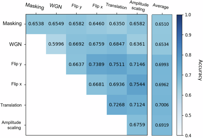
The matrix reveals the performance of models under the combination of different augmentation methods. The right column illustrates the average leak detection performance cecombined with other methods.
Regarding average accuracy, the masking (65.10%) and adding white Gaussian Noise (WGN) (65.34%) reach lower accuracy. It might be explained by the masking operation disrupting the temporal dependencies and continuity of the signals, leading to the loss of essential frequency components. However, these features are crucial for acoustic leak detection. On the other hand, for WGN, the original signals may already contain natural noise. Adding the 0 dB WGN might bury or obscure the meaningful information in the signals. flip x (69.62%), flip y (69.93%), translation (70.06%), and amplitude scaling (69.19%) share close average accuracy. From an overall accuracy perspective, augmentation, amplitude scaling, and flip x demonstrate the highest performance, reaching 75.44% leak detection accuracy, followed by flip y and translation (75.11%). Comprehensively considering the above results, this study adopted flip x and amplitude scaling as the augmentation method for subsequent CL.
Model ablation
The model ablation experiments were conducted to evaluate the influence of the number of convolutional blocks on CL leak detection modeling. The experiments respectively consider five settings from two to six convolutional blocks. Figure 2 respectively depicts the results of the CL model with different architectures from accuracy, F1-score, and cross-entropy. Overall, it can be observed that as the number of convolutional blocks increases, various performance indicators of the model improve continuously. Regarding accuracy, as the number of convolutional blocks increases, accuracy significantly rises from 65.46% with two convolutional blocks to 79.47% (three blocks) and then gradually increases to 83.09% with four blocks. A bottleneck is encountered at five convolutional blocks with an accuracy of 91.29%, and further increasing the number of convolutional blocks to six does not result in a significant increase, with 91.61%.
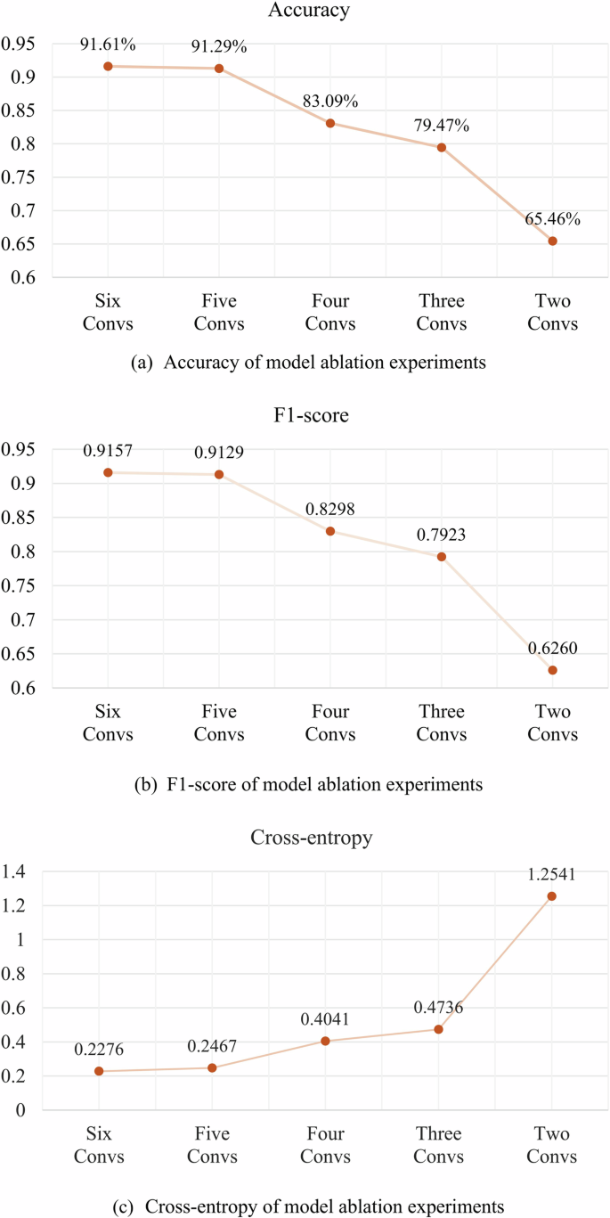
The figure compares the leak detection performance of models having different convolutional blocks. a, b indicate the leak detection accuracy and F1-score of the models. Both metrics gradually improve with the increase of the number of blocks. Similarly, (c) shows the cross-entropy of models, and the error increases with the decrease in the number of blocks.
F1-score shows a similar trend. Initially, the score is relatively low with two convolutional blocks (0.6260) and gradually increases to 0.9129 with five convolutional blocks, after which a bottleneck is encountered at six convolutional blocks (0.9157). The cross-entropy also follows this pattern. The model performs the worst with only two blocks. As the number of blocks increases, the loss gradually decreases, reaching its lowest point with five convolutional blocks (0.2467) and six convolutional blocks (0.2276).
Meanwhile, as shown in Fig. 3, t-SNE analysis was employed to assess the leak detection capability of five model architectures on the validation dataset. In Fig. 3a, the distribution of the original signals does not clearly distinguish between leak conditions, as samples from no-leak and leak are mixed. After the feature extraction of the CL model, the visualization result for the two-block model (shown in Fig. 3b) indicates a significant improvement in clustering performance. However, some of the samples remain mixed. However, a portion of the samples remain indistinguishable and exhibit overlapping characteristics. It can be attributed to the acoustic similarities between leak and no-leak samples, which show comparable characteristics due to factors such as signal attenuation. These similar acoustic features make it challenging for the model to distinguish leak conditions effectively.
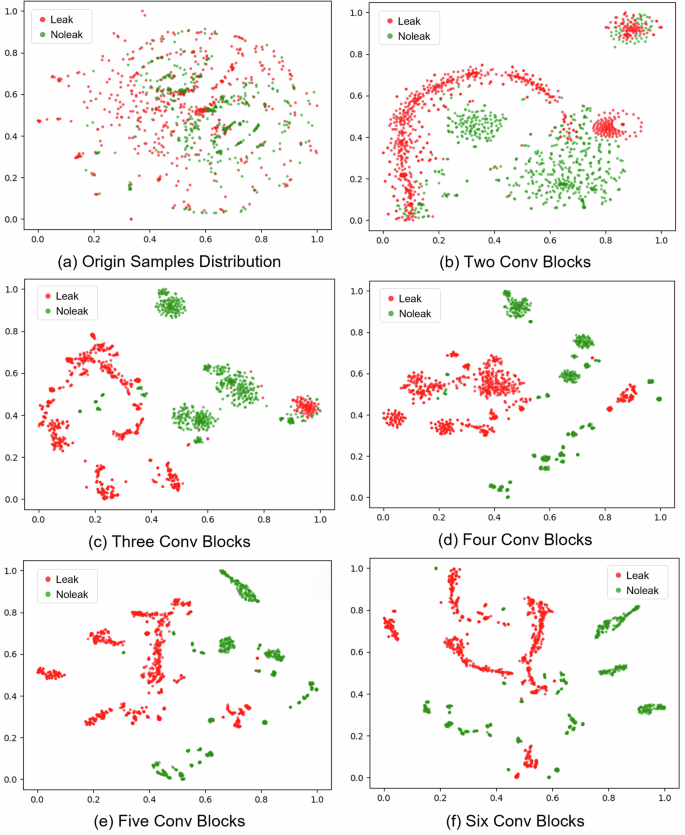
a Origin samples, b two, c three, d four, e five, and f six convolutional blocks. The figure illustrates the distribution of samples after different model feature extraction operations. a depicts the origin distribution of collected signals. Besides, (b–f) draws the distribution of feature vectors with different convolutional blocks, from two to six blocks.
Regarding the three-block model (shown in Fig. 3c), samples corresponding to different leak conditions form more concentrated clusters. Sub-clusters are also observed in the same leak condition. It may be attributed to collecting samples multiple times from various experimental sites, where samples obtained from the same site or exhibiting similar environmental factors are likely to be grouped into the same sub-cluster. This observation underscores the model’s robust fitting capability, distinguishing between leak and no-leak samples across diverse scenarios.
As shown in Fig. 3d, with the number of blocks increasing from four to five, the distance between signals of the same class decreases. At the same time, the differences between clusters from different leak conditions become more pronounced. Meanwhile, similar to the model performance metrics, the five-block model (Fig. 3e) and the six-block model (Fig. 3f) exhibit comparable leak detection clustering capabilities with close sample distributions. It suggests that as the model’s complexity increases with the number of blocks, its leak detection performance has likely reached a plateau, corresponding to the inherent complexity of the leak detection problem in this study.
In summary, the number of convolutional blocks significantly influences the performance of CL. Models with five or six blocks gradually perform better, displaying superior model metrics and feature extraction capabilities compared to models with fewer blocks. However, it is also noteworthy that continuously increasing the number of blocks does not always result in higher performance. The model reaches a performance plateau with five or six blocks, where their performance metrics are very similar. This phenomenon can be explained by the increased number of parameters in more complex models, which enhances their capacity to capture patterns, thereby improving performance as the number of blocks increases28. However, once the model’s complexity aligns with the problem’s complexity, additional increases in complexity contribute minimally to performance enhancement. Given that a simpler model with the same architecture can conserve computational resources and mitigate overfitting, this study adopts the model with five convolutional blocks as the primary architecture for experiments.
Comparison of labeled datasets with varying data volumes
To evaluate the influence of the labeled dataset volume on CL, a comprehensive experiment was conducted using different proportions of the labeled dataset: 5%, 10%, 15%, 20%, 25%, and 30%. The results of CL were then compared to the performance obtained from SL. Notably, CL and SL were trained using the same training dataset. Figure 4 illustrates the performance of models across different volumes of labeled datasets, evaluated through validation accuracy, F1-score, and validation loss. The CL model outperforms the SL model across all data volumes and metrics.
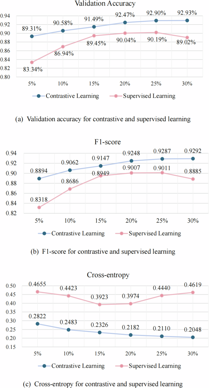
The figure compares the leak detection performance of models with different proportions of labeled datasets using SL and CL. a–c respectively depict the leak detection accuracy, F1-score, and cross-entropy of models using SL and CL. The CL outperforms SL across a wide range of data volume proportions.
For validation accuracy, the performance of SL improves with increasing data volumes, reaching a peak at 25% volume (90.19%). Meanwhile, CL’s accuracy continuously improves with more extensive data volumes, peaking at 30% (92.93%). CL achieves higher validation accuracy across all data volumes than SL, demonstrating superior performance and stability. Regarding the F1-score, SL shows an improvement with increasing data volumes, peaking at 25% (0.9011), followed by a slight decline at 30% (0.8885). In contrast, the F1-score for CL steadily improves with more extensive data volumes, peaking at 30% (0.9292). Thus, CL consistently outperforms SL regarding the validation F1-score across all data volumes. Regarding cross-entropy, SL exhibits an initial decrease as the data volume increases from 5% to 30%, but the loss begins to rise again after reaching a volume of 20%. Conversely, CL consistently demonstrates a decrease in validation loss with increasing data volumes, reaching its lowest point at a volume of 30% (0.2048). This consistent improvement highlights the superior performance of CL in minimizing validation loss compared to SL.
In summary, CL consistently outperforms SL across all metrics, including accuracy, cross-entropy, and validation F1-score. CL demonstrates superior performance and efficiency compared to SL at similar data volumes. The stability and efficiency of CL render it an effective learning method, mainly when there is a limited unlabeled dataset size.
Out-of-sample validation
Out-of-sample validation was employed to evaluate the generalization performance of the developed model beyond the training data. Therefore, a separate dataset, distinct from the training data, was collected from independent field sites to evaluate the effectiveness of CL in comparison to SL. Both CL and SL models were previously trained based on various volumes (5%, 10%, 15%, 20%, 25%, 30%) of labeled datasets.
Figure 5 depicts the outcomes of the leak detection models when applied to varying volumes of data. The evaluation metrics employed cross-entropy, F1-score, and accuracy. Based on the results, it is observed that a modest improvement in CL and SL model performance is evident when the dataset volume is increased from 5% to 30%. However, the volume of datasets does not significantly influence the performance of both CL and SL. Notably, this suggests that larger datasets may contribute to enhanced performance. Meanwhile, the metrics indicate that CL consistently demonstrates superior performance relative to SL across all metrics in out-of-sample validation. This finding highlights the potential advantages of leveraging unsupervised pre-training techniques, which may facilitate better generalization capabilities.
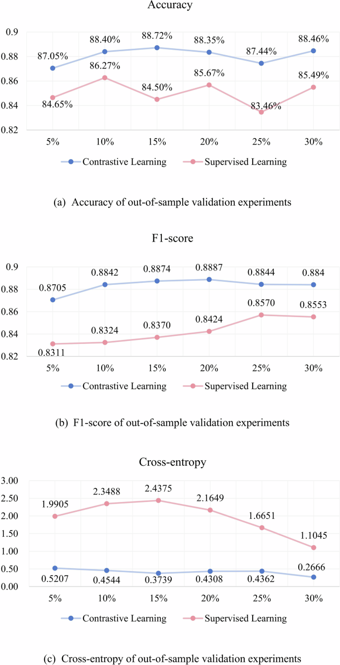
The out-of-sample validation performance of CL and SL models based on different proportions of label dataset. a–c respectively depict the leak detection accuracy, F1-score, and cross-entropy of models on unexplored sites. Most models reach promising and comparable leak detection capabilities.
Regarding accuracy, CL-based models achieve an accuracy range of 0.8705 to 0.8872, surpassing the SL-based models, which exhibit a range of 0.8346 to 0.8627. This trend is similar to the F1-score and cross-entropy metrics. Although SL results demonstrate slight improvements with an increase in the volume of training data, they remain generally inferior to the outcomes produced by CL, suggesting the robustness of CL approaches.
These findings suggest that models enabled by CL attain near-optimal performance, even when trained on a limited number of labeled samples. This capability underscores the potential of CL as an alternative approach for scenarios characterized by limited labeled datasets, thereby contributing to the broader advancement of ML-based leak detection methodologies.
Discussion
To address the shortage of labeled leak signals, this study explores the application of CL for leak detection in WDNs. The self-supervised nature of CL enables the utilization of unlabeled data, thereby reducing dependence on expensive and time-consuming excavation work to verify actual leak conditions. First, field experiments were conducted to collect acoustic signals for subsequent CL modeling and evaluations. The model, comprising the encoder and projector, was initially trained on unlabeled signals. Then, the pre-trained encoder was fine-tuned for subsequent leak detection tasks. The proposed CL-based model’s capabilities were then demonstrated and evaluated through augmentation analysis, ablation analysis, comparison analysis, and out-of-sample validation.
The findings underscore the effectiveness of CL in capturing meaningful representations from unlabeled acoustic signals. Specifically, among five signal augmentation methods, the combination of flip x and amplitude scaling is recommended as the optimal data augmentation technique, facilitating the CL model’s ability to capture acoustic characteristics for leak detection. Ablation experiments were conducted to optimize the CNN, integrating t-SNE to illustrate the impact of model complexity on CL performance. Additionally, comparison experiments illustrated that CL models achieve higher accuracy than SL models in various limited-labeled dataset scenarios. The robustness of CL was further verified through out-of-sample validation and compared to SL, demonstrating the effectiveness of CL in leak detection.
Methods
This study emphasizes using a contrastive-learning-based approach for acoustic water leak detection in WDNs. Figure 6 illustrates a three-step framework for CL-based leak detection modeling, outlining the key stages involved in the proposed methodology.
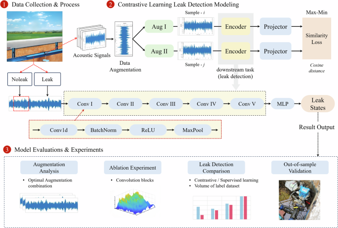
The figure shows the three-tier framework for contrastive-learning-based leak detection: data collection, contrastive learning leak detection modeling, and model evaluation and discussion.
The initial step in the framework encompasses the collection and processing of data. Acoustic signals from the WDNs are acquired using suitable sensors or devices. These signals serve as a valuable source of information for detecting the presence of leaks. Subsequently, the collected data is subjected to preprocessing and prepared for subsequent analysis. In the second step, the CL-based approach is applied to establish a self-supervised-CL-based model for leak detection. This approach leverages the principle of self-supervision. It trains the encoder using self-supervised learning, acquiring representations of the acoustic signals without relying on labeled data.
By pre-training the encoder, the model can capture crucial acoustic features and patterns that distinguish each acoustic signal, laying the foundation for effective leak condition classification. Once the encoder has been pre-trained, it is the foundational component for the subsequent leak detection task. Fine-tuning would be applied to adapt the model specifically for leak detection, further optimizing its performance. This fine-tuning process ensures that the model becomes specialized in accurately and efficiently identifying leak states by utilizing the features acquired during the CL phase.
Cross-entropy, leak detection accuracy, and F1-score are considered when evaluating the proposed model’s performance. The augmentation strategy should be optimized. Comparative analyses of leak detection performance are performed to assess the efficacy of the CL approach in comparison to SL. Additionally, ablation experiments are conducted to evaluate the influence of model architectures and gain insights into its impacts. t-SNE visualization represents the model’s ability to cluster and differentiate instances associated with different leak conditions. Furthermore, out-of-sample validation is undertaken to assess the generalization ability of the model when confronted with unseen data. The detailed procedures and outcomes of the steps above are depicted in the subsequent section of this study.
Data collection and process
Hong Kong, China, is a densely populated city with extensive WDNs. However, the average age of the pipeline network is over thirty years, leading to pipeline deterioration, leaks, and water supply instability. Therefore, it provides opportunities to collect the leak and non-leak samples for leak detection experiments. As depicted in Fig. 7, the research team deployed noise loggers in the chambers close to the potential leak points. The noise loggers are connected to the valve or pipeline to collect vibroacoustic signals caused by the leaks in the pipe. The signal collection is set at the sampling rate of 4096 Hz and lasts 10 s for each sample. To avoid the influence of external noise in leak detection, the signal collection occurred at midnight. For each leak site, the collection period would last several days, depending on work conditions, to ensure sufficient data volume and avoid unexpected noise.
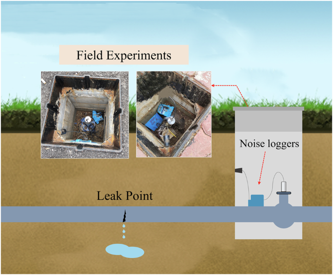
The figure shows the deployment plan of noise loggers on water distribution networks. The noise logger was deployed in the chamber to collect signals for subsequent modeling.
In total, 1004 samples were collected, including 439 leak samples and 565 non-leak samples. Each 10-s sample was divided into 1-s segments to enrich the dataset, considering the basic units. Ultimately, 4390 leak samples and 5650 no-leak samples were collected for subsequent modeling.
Acoustic leak detection modeling
CL is introduced to train the model in capturing the intrinsic feature and semantic details of the data32, thereby enabling the learning of representative representations. The pre-trained blocks enhance the model’s generalization and robustness capabilities33 in downstream tasks, including classification and fault detection. As depicted in Fig. 8, CL modeling procedures can be mainly divided into two phases: i) CL pre-training and ii) Leak detection modeling (downstream task fine-tuning).
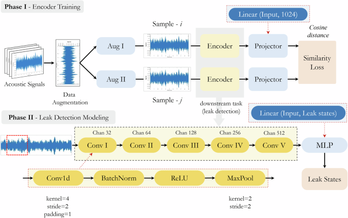
The contrastive learning training consists of two phases: contrastive learning-based pre-training and leak detection task fine-tuning. CNN is employed as the backbone for contrastive-learning-based leak detection modeling.
Figure 9 shows the conceptual framework for CL. The self-supervised CL utilizes unlabeled data and designs its supervisory signals to learn data representations, significantly reducing annotation costs. First, based on the existing sample x, the approach would generate negative and positive samples using different augmentation ((t sim tau) and (t^{prime} sim tau)), respectively, generating new samples, ({hat{x}}_{i}) and ({hat{x}}_{j}) to enhance the model’s understanding of data. For time-series signals, the basic augmentation tool includes Gaussian noise, time shift augmentation, pitch shift augmentation, jitter, and adjacent sample augmentation34,35. Generally, the two signals generated from the same sample are considered positive pairs, while signals generated from different samples are considered negative pairs. These augmentation operations can increase the diversity between samples, thereby helping the model learn more robust representations.
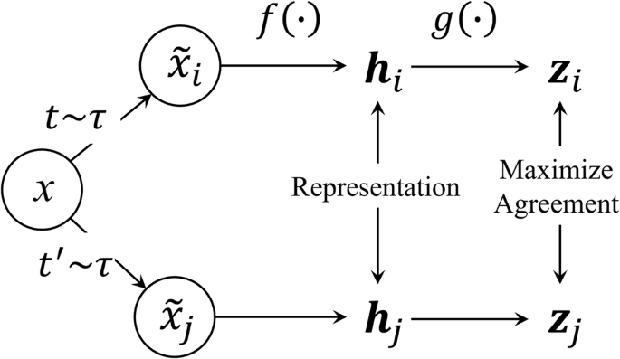
The infoNCE is employed to control the distance of signal pairs and help the model capture the representation of signals.
Subsequently, the basic encoder f (·) is utilized to project the input x into the representations h. Then, it is passed through the projection head g (·) to obtain the vector Z. The model is then generally trained using InfoNCE to maximize the consistency among positive pairs and minimize the consistency among negative pairs, as depicted
where ({rm{I}}) is the indicator function, it outputs 1 when (k,ne,j), while outputs 0 when (k=j).
The function sim () denotes the similarity score between two vectors. This study utilized cosine distance to measure the cosine of the angle between two vectors, effectively capturing relationships between feature representations in high-dimensional space36. τ is a temperature parameter that controls the sharpness of the distribution, N is the number of batch sizes, and zi and zj denote the signal pairs.
This study’s prominent architecture of CL consists of an encoder and a projector. CNN is employed as the backbone of CL because of its proficiency in processing sequential data, including seismic signal37, time-series data38, and speech recognition39. The convolutional layers are the core of CNNs that utilize learnable filters or kernels to extract the local and global features from input signals40,41. The convolutional layers enable the model to capture local patterns and learn representations at different feature levels. The process within the convolutional layers is depicted as:
where ({K}_{i}) is the i-th kernel, and ({b}_{j}) is the bias, x is the values within the kernel, and y is the kernel output.
Specifically, as illustrated in Fig. 8, the encoder consists of several convolutional blocks, processing and extracting features from input signals. Each block begins with a one-dimensional convolutional layer (Conv1d) with a kernel size of 4, stride of 2, and padding of 1, allowing the model to capture local patterns in the input signal while maintaining dimensionality40,41. Following the convolutional layer, batch normalization is applied. This step stabilizes and accelerates the training process by normalizing the inputs of each layer42. Subsequently, Rectified Linear Unit (ReLU) activation function is used to introduce non-linearity into the model, enabling it to learn complex patterns in the data43. After that, max pooling layer (MaxPool1D) with a kernel size of 2 and a stride of 2 is employed. Max pooling reduces the dimensionality of the feature map. It mitigates the impact of data noise, thereby reducing the computational complexity and aiding in capturing dominant features in the input signal40. Each convolutional block progressively projects the channels from the input dimension to higher dimensions. Specifically, the channels are projected from 1 to 32 in the first block, then 64 in the second block, and 512 in the subsequent blocks. This gradual increase of the model depth allows the model to capture high-level features from acoustic signals.
Following the final convolutional block, a projector layer is connected. The projector is the fully connected layer that maps the high-dimensional features extracted by the convolutional blocks into a lower-dimensional space suitable for similarity measurement. This component is critical for tasks such as CL, where accurately measuring the similarity between pairs of signals is essential. The projector transforms the input vector into the 1024-dim vector. By utilizing InfoNCE loss (Eq. (5)) and extracting critical features from the signals, CL enhances the encoder’s feature capture capabilities and provides valuable insights for subsequent tasks.
After initial CL pre-training, fine-tuning would be conducted, regulating the encoder to fit into the leak conditions. It is worth noting that the encoder is connected to the Multilayer Perceptron (MLP), therefore outputting the leak conditions of input samples. The settings of downstream modeling would be adjusted according to the experiment’s purposes.
Model evaluation and experiments
In this section, the evaluation and experimental results of the proposed model for leak detection are presented. A comprehensive set of experiments was conducted to assess the performance and effectiveness, including data augmentation experiments, model ablation experiments, comparison of labeled experiments, and out-of-sample validation.
Regarding data augmentation experiments, CL requires applying data augmentation methods to generate positive and negative samples for in-depth feature captures. The synergy of augmentations would greatly influence the performance or effectiveness of CL. Therefore, conducting a series of experiments to explore the optimal combination of augmentation methods and reach a higher accuracy is crucial. Due to limited computational resources and feasibility, this study excluded ML-based augmentation methods, such as autoencoders and GANs. Instead, considering the augmentation approaches employed in previous studies44,45, this study focused on signal-based augmentation methods, including masking, WGN, flip y, flip x, translation, and amplitude scaling. Detailed explanations of these augmentation methods are provided in Eqs. (7) to (12).
1) Masking (Eq. (7)): The operation randomly occludes or masks out a portion of the input signal with probability p. This can improve the model’s robustness to partial data missing.
2) Adding WGN (Eq. (8)): The operation overlays the input signals with random noise following Gaussian distribution (N(0,sigma )). This study generated the WGN at 0 dB46,47,48, enhancing the model’s robustness to noisy inputs.
3) Flipping along the y-axis (Flip y, Eq. (9)): This operation vertically flips the input signals, increasing the model’s adaptability to vertical variations.
4) Flipping along the x-axis (Flip x, Eq. (10)): The operation horizontally flipping the input signals. This can enhance the model’s adaptability to horizontal variations.
5) Translation (Eq. (11)): The operation randomly shifts i units of the input signals in the spatial or temporal dimensions. The i is a random value ranging from 1 to the total length of the input vector minus one. This operation might improve the model’s robustness to changes in the input positions.
6) Amplitude Scaling (Eq. (12)): The operation randomly scales the amplitude or magnitude of the input signals through the coefficient (alpha), enhancing the model’s robustness to changes in input amplitudes. In this study, the factor σ was set to 1.1.
Meanwhile, model ablation is conducted to understand the contribution and significance of different components within the model architecture. By systematically removing or altering specific parts of the model, experiments reveal the impact of these changes on overall performance to optimize the model architecture.
This study employed ablation experiments to evaluate the leak detection capacity of models under different amounts of convolutional blocks. The optimal convolutional blocks were selected based on the leak detection results. Specifically, as shown in Fig. 10, the ablation experiments were conducted on models with different numbers of convolutional blocks, including i) Two conv blocks. ii) Three Conv Blocks. iii) Four Conv blocks. iv) Five Conv bloks. v) Six Conv blocks. Each model was trained with CL and the 10% labeled dataset for downstream leak detection training.
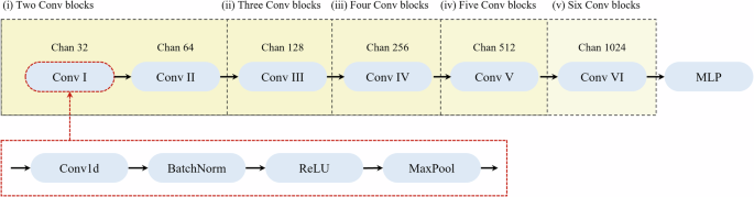
The experiments start with a model having two convolutional blocks, and each subsequent experimental setup increases the number of blocks by one.
Regarding the comparison of labeled datasets, CL enables the model to be trained using limited label samples. Experiments employed CNN as the backbone for leak detection modeling to demonstrate this point. CL and SL were used to train the model under different proportions of labeled datasets. Specifically, during experiments, a small proportion of the labeled dataset was applied for leak detection training, while the remaining part was used for validation. Specifically, this study extracted 5%, 10%, 15%, 20%, 25%, and 30% of the labeled dataset to train the model using different learning methods. The objective is to evaluate the effectiveness of CL in leveraging unlabeled acoustic signals and achieving comparable or superior performance with a smaller amount of labeled data. Besides, the comparison also reveals the influence of data volume on the leak detection performance.
Out-of-sample validation represents a critical methodology to assess the model’s performance on novel and unseen data, distinct from the data used during its training phase. This evaluation determines the model’s ability to accurately predict previously unencountered data instances. In the specific context presented, supplementary field experiments with the same experiment setting were conducted on WDNs. Consequently, an independent dataset was meticulously assembled, comprising 670 samples indicative of leaks and 890 samples denoting non-leak conditions. Notably, these samples were obtained from unexplored sites, ensuring their novelty and relevance for the evaluation process. Through this rigorous evaluation, the robustness of the model is thoroughly examined, with particular attention given to its capacity for accurately classifying signals associated with leak conditions in unexplored real-world scenarios.
Responses