Assessing the effectiveness of interdependent corporate sustainability choices

Introduction
Companies in energy and energy-intensive industries provide essential services to modern societies1,2. However, their business activities are also the primary sources of greenhouse gas (GHG) emissions3,4,5, and depletion of natural resources6,7. Therefore, balancing the profitable production of goods and services with a reduction of the environmental externalities of business operations of companies in the energy and energy-intensive industries is a central challenge in the transition to a low-carbon economy8,9,10.
Addressing this challenge requires effective sustainable decision-making processes which, in turn, hinge upon the ability to identify environmental management practices and organisational changes that align companies’ economic interests with broader environmental needs10,11,12, e.g., the optimum levels of investment in maintenance capital expenditure, sustainable growth opportunities, and stakeholder engagement activities. However, identifying effective changes in business approaches to environmental sustainability issues is challenging due to the strong interconnections among corporate choices of investments in strategic actions and the heterogeneous implications of choices’ interdependency for companies’ integrated financial and environmental performance (henceforth “integrated performance”).
From a theoretical standpoint, it is well-recognised that understanding the importance of heterogeneous impacts of trade-offs and interconnections of corporate choices on companies’ integrated performance is crucial for effective sustainable decision-making13,14,15,16. For example, finding the optimum balance between investment in decarbonisation strategies and direct return of capital to shareholders, a typical issue for energy companies17, is contingent on several other firms’ characteristics, financial choices, and macroeconomic conditions, such as firms’ revenue, debt levels and environmental policy landscapes. Similarly, budgeting constraints and capital structure choices influence investment in sustainability projects heterogeneously depending on firms’ exposure to Environmental, Social and Governance (ESG) risks, volatility, and discount rates18. However, choice interdependency is systematically overlooked in empirical sustainable finance, management, and strategy science studies, which are primarily based on linear assumptions and, therefore, discount complex heterogeneous effects of corporate actions on firms’ value.
Against this backdrop, the objective of this work is to develop an empirical framework to assess the effectiveness of corporate sustainability choices in determining companies’ integrated performance by explicitly and systematically accounting for their interdependencies. Applying our framework to a sample of large global publicly traded corporations in the energy and energy-intensive industries, we empirically quantify the level of choices’ interdependency and estimate their effectiveness in increasing firms’ financial and environmental value. We then investigate the extent to which corporate actions deviate from hypothetical quasioptimal (“satisficing”) choices and identify the source of deviations. Overall, our work provides a framework for assessing companies’ contributions to the low-carbon transition and can be used to guide changes in corporate decision-making processes.
Results
Theoretical background and overview of the framework
Before presenting our results, we provide a theoretical overview of our framework and how it differs from previous studies that investigate the role of choices’ interdependency on corporate outcomes. Then, we provide a qualitative description of our empirical approach. Further details on the methodology can be found in ‘Methods’ and the Supplementary Information.
Frameworks that study the impact of interactions among choice variables on corporates’ outcomes in organisation studies are often inspired by Wright’s notion of fitness landscapes19. In particular, most previous works build on ref. 20, which, in turn, builds on Kauffman’s NK model21 that we here briefly summarise. Broadly speaking, the fitness of a system (e.g., an organisation) is proportional to its likelihood of survival within a given environment, and it is a function that maps attributes (e.g., a series of corporate choices) to outcomes (e.g., a firm’s performance). While attributes can, in principle, be in one of several states, in the original NK model and most of its applications, each of the N attributes can exist in either of two states, e.g., zero or one22. The interdependencies between the attributes are regulated by a variable K, i.e. the higher the value of K, the higher the interactions between the different attributes N. K plays a crucial role in the NK model since it correlates to another important property of fitness landscapes, their surface ruggedness. Like rugged surfaces, rugged landscapes are those where nearby states can differ significantly in fitness value due to the presence of interactions among attributes. Ruggedness is an important property of NK models because it strongly influences agents’ dynamics on the landscapes23,24.
The NK model has been particularly successful in the organisation, strategy and management literature because it incorporates several concepts that are relevant for effective decision-making processes25. Most importantly, system-level outcomes depend on the interactions between multiple components of the system26. Strong interactions (high ruggedness) make managerial decision-making complex because combinatorial tasks become significantly more difficult when changes in one choice variable can have consequences on its interconnected components27.
Identifying financial and nonfinancial choices that align companies’ economic interests with broader environmental needs is a combinatorial task with nontrivial interactions among choice variables. Hence, it is a problem that can be studied under the lens of fitness landscape analysis. Against this backdrop, in this work, we conceptualise an organisation as a complex adaptive system evolving in highly uncertain economic, policy, and business environments. Changes in corporate sustainable behaviours (i.e., the specific choices of sustainability actions and goals) can be seen as adaptive (non-adaptive) steps that increase (decrease) companies’ fitness within their environment. We consider the fitness of an organisation—its likelihood of survival—to be proportional to the integrated financial and nonfinancial value it creates. In this work, we use idiosyncratic price returns to measure the value generated to investors and GHG emissions reduction capabilities to measure the value generated to the environment, albeit the framework, conceptually, can be extended to other stakeholders if accurate measurements of the value returned to them can be obtained.
Our study differs from previous works in two main aspects. First, our framework is purely empirical. We start from observations of N attributes (sustainability choices, financial characteristics, and fixed effects) and we then estimate, non-parametrically, the level and structure of the interactions among them (i.e., the variable K in the NK framework and the underlying data-generating process). Therefore, the structural properties of the landscape, such as the relative importance of each attribute to the overall fitness and the level of interactions among attributes, are empirical characteristics of our sample, not properties of a model. Indeed, most of our empirical results will focus on analysing these characteristics, which are important for the potential implications of our understanding of firms’ decision-making processes and experimentation in a highly rugged empirical landscape20. This is in stark contrast with most previous works in organisation and management science that are mostly based on theoretical modelling and numerical simulations25,27,28, with only a few exceptions that involve experimentation (see refs. 27,28, for example).
Second, to the best of our knowledge, no previous empirical study has used fitness landscape theories to analyse corporate sustainability choices and their performance implications. While our framework uses fitness landscapes as sensitising concepts29, it provides a new lens to study this central problem in sustainable business studies, a lens that explicitly accounts for the complexity involved in sustainable decision-making. To showcase the possible implications of our framework, in the last section of this manuscript, we provide an application to illustrate how our approach can be used to identify deviations of corporate sustainability choices from, hypothetical, quasioptimal (“satisficing”) behaviours.
In the following two sections, we provide an overview of our empirical process, which is divided into two steps: (1) an estimation and characterisation of the fitness landscape to quantify the level of choices’ interdependency and their relevance for firms’ integrated performance and (2) an exploration of the landscape to search for quasioptimal solutions and identify gaps between observed and quasioptimal choices. For ease of exposition, the description of our framework is mostly qualitative. Technical details can be found in Supplementary sections S2 and S3.
Overview of the study: estimation of the fitness function
We start by representing the integrated financial and environmental performance (({mathcal{P}})) of a company as a function (({mathcal{F}})) of its sustainability behaviour (({mathcal{B}})), financial behaviour and assets characteristics (({mathcal{X}})), and fixed effects (({mathcal{S}})). Namely:
Where ({mathcal{F}}) is the fitness function to be estimated empirically. We impose a time lag between the dependent and independent variables because we do not expect that the effects of sustainability and financial choices are reflected in contemporaneous prices or sustainability outcomes. Indeed, the effect of behaviour on emissions can even be studied on multiple lags, but for simplicity here we only focus on a one year lag. The performance ({mathcal{P}}), our objective function, is either a financial measure (f, yearly idiosyncratic equity returns), an environmental measure (e, negative changes in GHG emissions), or a mixture of the two (see Data for the definitions of the variables):
Where ({mathcal{W}}) is the weight given to the financial performance and ranges between zero and one. For (0 < {mathcal{W}} < 1), ({mathcal{F}}) is a return measure that weight returns to shareholders with the value returned to the environment and local communities. ({mathcal{W}}=0,1) instead corresponds to a purely environmental and financial return measure, respectively. We are interested in studying the characteristics of fitness as a function of the combination of financial and environmental performance because we do not have a clear prior expectation for the objective of companies’ sustainable choices. We expect a trade-off between financial and nonfinancial objectives because sustainability can have economic costs and advantages30, but the relative importance of financial and environmental considerations in this trade-off is unclear. Therefore, to limit the number of ex-ante assumptions in our analyses, we will present all our results as a function of ({mathcal{W}}), the weight given to the financial performance.
In (1), we assume that the performance of an organisation is a function of its sustainability behaviour (({mathcal{B}})) and a set of companies’ characteristics (({{mathcal{X}}}_{t},{mathcal{S}})). The sustainability behaviour of a company is defined as the particular combinations of actions that a company implements in a given year to meet sustainability goals. In section ‘Behavioural dataset’ we provide a detailed explanation of the data we use to characterise companies’ behaviour. Briefly, the dataset is generated using large language models to analyse sustainability reports and extract sustainability initiatives. These initiatives are then categorised in nine types of actions (e.g., investment in R&D projects, replacement of existing assets) and their most closely related Sustainable Development Goal (SDG). The SDGs are subsequently grouped into environmental challenges as explained in section ‘Behavioural dataset’. The company-year combination of all actions and challenges form a particular configuration of a matrix called behavioural matrix, ({mathcal{B}})31, that characterises the sustainability behaviour of a company. Figure 1 shows the Sankey diagram of the matrix after aggregating data over the full sample. Notice that the activities considered in this work are not exhaustive. They focus exclusively on actions that address core business operations and exclude stakeholder engagement activities. This is a necessary limitation to manage the dimensionality of the problem and it should be addressed in future works.

The figure shows the Sankey diagram of the behavioural matrix that characterises the sustainability behaviour of companies in our sample. The full behavioural matrix is shown in Supplementary Fig. S2. Each line in the diagram represents an action (left) undertaken to address one of the three macro environmental challenges (right). The colours of the macro challenges on the right hand side are based on the most prevalent actions implemented to address them.
While the behavioural matrix keeps track of the total number of company-year initiatives; in the following, we characterise the sustainability behaviour with an on-and-off (binary) allocation of initiatives. That is, we cast the behavioural matrix, ({mathcal{B}}), of each company and year into a binary matrix where each entry (i.e., each combination of actions and sustainability challenges) takes the value of one if the company has taken more initiatives than the 75th percentile of the yearly distribution of initiatives. Results are robust to different choices of the threshold, as we will show in the section ‘Model validation and performance implications of sustainability choices’. We call this binary allocation matrix ({mathcal{A}}), and therefore ({{mathcal{P}}}_{t+1}={mathcal{F}}({{mathcal{A}}}_{t},{{mathcal{X}}}_{t},{mathcal{S}})+{epsilon }_{t}). Here we focus on binary allocations for three reasons: (1) in the dataset we do not discriminate initiatives based on their complexity and costs, we simply assume that if there has been an activity implemented to meet a particular SDG target then there was a managerial effort behind the decision which is here considered as part of the behaviour; (2) optimisation processes to identify quasioptimal solutions are more likely to converge towards the relevant local optima as the search space is significantly smaller; (3) the vast majority of previous studies in organisational adaptation, corporate strategy and theoretical works on NK models, have also focused on binary allocations20,32,33,34.
In the fitness function (1) we also account for several companies characteristics (({{mathcal{X}}}_{t},{mathcal{S}})) including Size, Invested Capital, tangible assets over total book assets (Tangibility), capital structure choices (Market Leverage, dividends per share, shares issuance and buyback), time and geography fixed effects, see section ‘Fundamental, market, and environmental data’ for the definition of the variables and section ‘Model specification’ for an explanation of their role in the model. To estimate empirical fitness landscapes (({mathcal{F}})) we use random forests with a feature selection step in the cross-validation. In Supplementary section S2 we provide a discussion of the implication of different estimation strategies.
Here we provided an overview of the landscape estimation process. In the next section, we provide a qualitative overview of the search process for quasioptimal solutions over the landscape. In Supplementary section S3 we provide quantitative details.
Overview of the study: exploration of the landscape
Our objective function (hat{{mathcal{F}}}) in (1) is a fitness function that maps financial and nonfinancial choices as well as firms’ characteristics to the fitness (performance) of a company. Focusing on nonfinancial choices, the set of all choices of sustainability actions and goals (sustainability behaviours) and their associated performance values creates a sustainability fitness landscape (henceforth “fitness landscape”) as schematically shown in Fig. 2. The landscape is made of peaks, troughs, and valleys. Observed behaviours are located somewhere across the landscape (e.g., the blue sphere in Fig. 2a), and our task is to find the closest fittest region of the landscape (closest peaks) that a focal company can reach under costs constraints, implemented here as a constraint on the difference between the number of initiatives of the solutions in the fittest regions and the number of initiative of the focal firm. To search optimal solutions over the landscape we use genetic algorithms (GA) as explained in Supplementary section S3, which also provides greater details on the process.
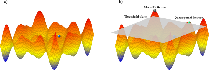
The figure provides a visual aid to illustrate our framework. a A simplified sustainability fitness landscape. The z-axis is the performance measure, hence peaks represent local and global optima. The x and y axes are the behavioural dimensions. The blue sphere represents the position of a hypothetical company on the landscape. In our search process we start from the proximity of the blue sphere, and we search a quasioptimal solution, which is the closest solution that lies above the cost constraint represented by the grey plane in (b) (e.g., the green sphere).
Cost constraints are a crucial feature of our framework. While the theoretical local optima we are searching for are local peaks on the landscape, our final solution (i.e. the final optimal behaviour) will not necessarily lie on any of the peaks. Indeed, if the search process finds a solution that is within a reasonable margin of the local optimal fitness, but significantly closer to the observed sustainability behaviour (in terms of cosine similarity), we will choose the closest solution rather than the fittest. This choice is in line with the behavioural view of strategic management, which assumes that sub-optimal outcomes are embraced by the company if they are above a minimum level35. The choice also aligns with Simon’s satisficing principle36, which states that under bounded rationality, agents facing complex tasks must do with satisficing solutions37. Graphically, one can imagine drawing a plan in the landscape which is within an ϵ from the global optima and accepting all solutions above the plane (whether on a peak or not). Among all these solutions, we then pick the closest to the observed behaviour as shown in Fig. 2b. In what follows we will call these “satisficing” solutions “quasioptimal” solutions.
The fitness landscape lives in a ((| {mathcal{A}}| +| {mathcal{X}}| +| {mathcal{S}}| )+1) dimensional space. However, in our process, we only search for quasioptimal allocations of actions and goals while keeping all the other variables (financial decisions and exogenous factors) fixed at their observed values (in Discussion we discuss the implications of this choice). That is, we fix the values in the (| {mathcal{X}}| +| {mathcal{S}}|) dimensions and search over binary combinations in the remaining (| {mathcal{A}}|) dimensions (i.e. ({2}^{| {mathcal{A}}| }) possible allocations). Hence, although the landscape itself is the same for every company and it is estimated over the full sample, the constrained quasioptimal behaviour for any given company can live around different peaks depending on the value of the fixed dimensions (i.e., on the idiosyncrasies of the companies), as also discussed in Supplementary section S2. Notice as well that here we present an analogy with fitness landscapes only for ease of exposition. In reality, given the environment-dependency of sustainability behaviours and their pay-off, it would be more appropriate to refer to our function as a fitness seascape, a concept introduced in ref. 38 to describe time-dependent selection processes in non-equilibrium adaptation dynamics. Indeed, in our analysis the fitness landscape does vary in time since we carry on the estimation on a rolling basis to account for yearly changes in business and policy environments (see Supplementary section S3).
Finally, we would like to stress that given the number of dimensions in the search space, and the approximations we made to accept solutions that are not necessarily on the global or any local peak, there is no guarantee that the final quasioptimal behaviours are close to being optimal in the classic sense of Pareto optimality. Therefore, our optimisation approach should be seen as a guided search for more fitted or satisficing choices rather than a rigorous mathematical approach. We discuss this critical point in further depth in the ‘Discussion’. We now turn to the presentation of the results.
Model validation and performance implications of sustainability choices
To present our results we start with an analysis of the validity of our empirical specification, and an investigation of the importance of companies’ sustainability choices, and their interdependency, in determining integrated performance. Then, we use our framework to identify deviations in companies’ sustainability choices from hypothetical quasioptimal decisions.
Our framework requires estimating fitness functions on empirical data, and then iteratively evaluating the functions on unobserved behaviours. Hence, we start our analysis by evaluating the generalisation skills of our model as explained in Supplementary section S4. Results are shown in Supplementary Fig. S4, which show the distribution of out-of-sample correlation coefficients between predicted and observed performances in a series of validity tests over random sub-samples. The generalisation skills of the model are generally high for the task at hand (ρ ~ 0.3), and, importantly, higher than those of a linear model evaluated on the same sub-samples, as shown in Supplementary Fig. S6.
The behavioural dimensions account for ~30% of the total feature importance in the model, suggesting that changes along these dimensions have a substantial impact on integrated performance (Supplementary Fig. S5). However, feature importance analyses provide limited information on the economic significance of the impact of the empirical choices on performance. Hence, to quantify this impact, we compare the performance implications of companies’ choices with the implications of random choices sampled as explained in the section ‘Validation and randomisation tests’. Results are shown in Fig. 3. The panel shows that the sustainability choices made by companies in our sample are associated with a higher performance than what the same companies would have achieved had they randomly allocated initiatives across actions and goals. The effects are small (20–100 basis points) but statistically significant, and the results are supported by the robustness analyses shown in Supplementary Figs. S8 and S9.
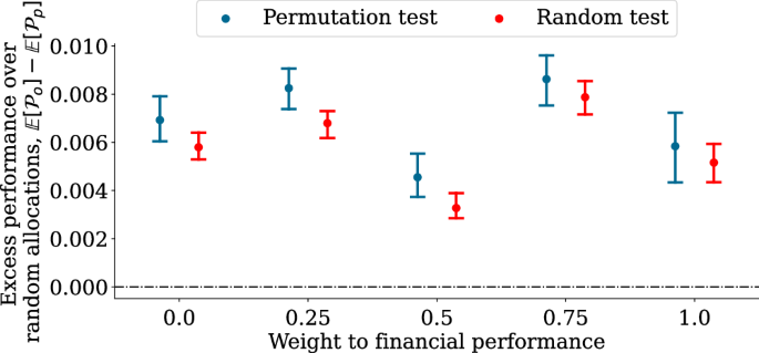
The Figure shows the results of the randomisation tests described in the section ‘Validation and randomisation tests’. The y-axis is the difference between the expected performance of a company and the expected performance of the same company under the permutation (blue) and constrained randomisation (red) tests. Error bars are 1.96 times bootstrapped standard errors of the medians.
Interdependent choices and estimation of performance gaps
Our results suggest that corporate sustainability choices have a measurable impact on integrated performance. In this section, we measure the extent to which the impact depends on choices’ interdependency. Supplementary Fig. S6 shows that non-parametric models are able to predict out-of-sample performances substantially better than linear models. This result suggests that the data-generating process includes interactions and nonlinearities, which cannot be captured under linearity assumptions. In the language of fitness landscape analysis, this result suggests that the underlying landscapes are rugged since ruggedness emerges from interactions among attributes (features) on the landscapes. To confirm this hypothesis, we explicitly estimate the ruggedness of the landscapes using the methodologies described in the section ‘Empirical ruggedness’. That is, we use the correlation of fitness effects of one or multiple mutations as proposed in ref. 39 (hereafter 1 − γ) and the r/s ratio40. The first measure characterises ruggedness across the behavioural dimensions. The second measure also includes interactions with and within financial choices.
Figure 4a shows the ruggedness (1 − γ) as function of the number of mutations. The black dotted line shows the theoretical expectation from a smooth (non-epistatic and purely additive) landscape. The panel shows that ruggedness increases as a function of the number of mutations, which is a typical trend in NK models with K > 039. However, the baseline values of 1 − γ for a few points mutations are low, suggesting a low level of interaction effects within the behavioural dimensions. Figure 4b shows the value of r/s as a function of the performance measure. The estimated values of the r/s ratio imply large ruggedness levels and, therefore, substantial interactions when accounting for financial choices. As a frame of reference, a House-of-Card (HoC) model, which is a completely random landscape with r/s → ∞ for N → ∞41, with the same number of dimensions of our empirical framework and same variance of the empirical fitness, has an average r/s ratio of ~12 (black dotted line).
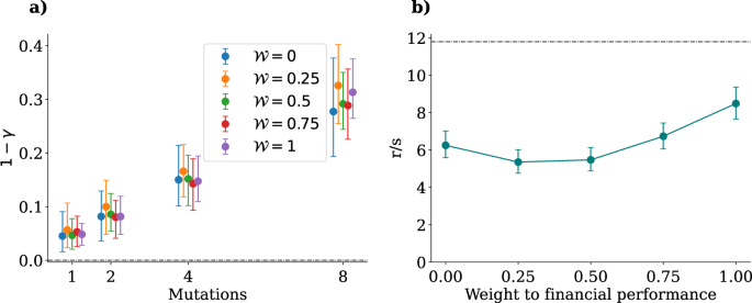
a The average value of the ruggedness within behavioural dimensions (y-axis) as function of the number of mutations (x-axis). In this panel, ruggedness is measured as 1 − γ as explained in the section ‘Empirical ruggedness’. The colours of the bars denote the different performance measures as shown in the legend. b The ruggedness measured using the r/s ratio (y-axis) as function of the performance measure (x-axis). The black dotted line in the panel shows the r/s ratio for the House-of-Cards model. Error bars are 95% bootstrapped confidence intervals.
Note that while we report the ruggedness values for each landscape (performance measure), we caution against drawing conclusions from comparing these values. The comparison could be misleading because the nature of the noise processes in the emission and financial measures are different, and ruggedness measures are strongly influenced by the origin of the noise in the data-generating processes40. In Supplementary section S5, we discuss this point in further depth.
Given the ruggedness of the landscapes, it is unlikely that the optimisation process converges to global optima42. However, we can still analyse the characteristics of the solutions that are closest to the observed behaviours under cost constraints (quasioptimal solutions, green sphere in Fig. 2) and their relationship with observed performances. Figure 5a shows the differences (performance gap) between the expected performance of the model under companies’ choices and the performance associated with hypothetical quasioptimal choices, across the performance measures (x-axis). Importantly, the performance gap between companies’ sustainability choices and their quasioptimal counterpart is, on average and in absolute value, substantially larger than the gap generated by differences between observed choices and random allocation of actions (Fig. 3). In Supplementary Fig. S11 we show that, while quasioptimal solutions are characterised by a larger number of initiatives (twice as many, on average, as the empirical allocations), the source of out-performance is likely the particular allocation structure, not the total effort. Interestingly, we have found that the bulk of the distributions (the interquartile range) of performance values in the quasioptimal regions are all positive, i.e., conditioning on the observed assets’ characteristics and financial choices, behavioural changes can allow companies to escape low-performance regions (Supplementary Fig. S10).
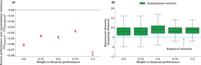
a Illustrates the gap between the expected performance of the model under companies’ choices and the performance associated with hypothetical quasioptimal (“satisficing”) choices. Error bars are 95% bootstrapped confidence intervals. b The distribution of the behavioural diversity of the quasioptimal solutions (green) and the empirical observations (blue line). Behavioural diversity is defined as Hamming distance across binary allocations. The middle lines of the box plots are median lines, and the edges of the boxes are the quartile range: the 25th and 75th percentile.
Figure 5b shows the behavioural diversity of quasioptimal solutions (green) versus the behavioural diversity of empirical observations (blue line). Behavioural diversity is defined as average differences (in terms of Hamming distance between binary allocations) of the behaviours of companies across the population. The panel shows that quasioptimal solutions are significantly more heterogeneous across companies than empirical behaviours, i.e., empirically, we observe a substantial degree of similarity across companies’ choices, while solutions in higher performance regions in the landscapes are characterised by a greater diversification of behaviour across the sample.
Identification of behavioural gaps
The performance gap shown in Fig. 5 provides an estimation of the potential benefits of effective changes in corporate sustainability choices. However, it does not inform us about the type of changes that need to be implemented to gain those benefits. To identify effective changes, we now study the gap between the sustainability choices of companies in our sample and the choices associated with the quasioptimal solutions, what we call the behavioural gap (see section ‘Estimations of behavioural gaps’ for a description of the estimation process). First, we notice that, in our empirical landscapes, there is a strong (conditional) correlation between distances in the behavioural space and companies’ performance (see Supplementary section S6 and Supplementary Table S3). That is, within the same landscape, companies closer to quasioptimal behaviours exhibit better performance. In Supplementary section S7, we show that while the correlation between companies’ performance and distances in the behavioural space is required to draw meaningful conclusions from the observations of behavioural gaps, in rugged landscapes, this correlation is not guaranteed.
Figure 6 shows the full distribution of the behavioural gaps across companies in our sample. Supplementary Fig. S12 and Supplementary Table S4 show the gaps aggregated at the population level and their statistical significance, as explained in the section ‘Estimations of behavioural gaps’. Positive (negative) values in the figure indicate average under (over)-investment, of our sample of companies, in a particular environmental challenge (top) and empirical mechanism (bottom) with respect to the quasioptimal solutions. The empirical mechanisms are defined in section ‘Data’ and follow a similar categorisation as the one suggested in ref. 12.
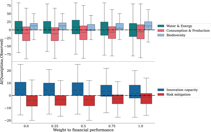
The figure shows the full distribution of the differences between the relative efforts of companies in our sample and the relative effort of quasioptimal solutions, along the environmental challenges (top figure) and empirical mechanisms (bottom figure) by performance measure (x-axis). Positive values indicate under-investment and negative values indicate over-investment with respect to the quasioptimal solutions (see section ‘Estimations of behavioural gaps’). The middle lines of the box plots are median lines, the green triangles are means, and the edges of the boxes are the quartile range: the 25th and 75th percentile.
The figures show that, on average, companies over-invest in sustainability initiatives aimed at addressing sustainable consumption and production challenges (top figure) as well as risk mitigation activities (bottom figure). On the other hand, we have found substantial average under-investments in innovation capacities, biodiversity, and water and energy challenges. Importantly, most of the deviations from quasioptimal behaviours are statistically and economically significant, and the signs of the behavioural gaps are consistent across the performance measures.
Discussion
Identifying the extent to which the sustainability choices of large global corporations in energy and energy-intensive sectors effectively increase firms’ integrated performance, and what type of choices would lead to better outcomes, is crucial for assessing companies’ contributions to the sustainability transition, and driving changes in corporate decision-making processes. In this work, we developed an empirical framework to identify the performance implications of companies’ sustainability choices and their deviations from hypothetical quasioptimal decisions. Here, we discuss the implications of our results, the limitations of our study and opportunities for further research.
First, we have found that corporate sustainability choices have a measurable impact on companies’ integrated financial and environmental performance. That is, the behavioural dimensions play a significant role in the model, and the integrated performance implied by observed behaviours are, on average, larger than those expected from random allocations of actions across sustainability challenges (Fig. 3). This result, which is robust to different randomisation strategies, suggests that, on average across our sample, sustainable management practices do not result from random investments across sustainability areas but instead emerge from effective decision-making processes. However, it is important to notice that, while statistically significant, the differences between the performance associated with empirical and random allocations, are economically small (20–100 basis points on average).
Second, we have found that empirical sustainability fitness landscapes are rugged (i.e., are shaped by interactions among companies’ choices), and the ruggedness is greater when we account for interactions across all the dimensions (behavioural and financial, Fig. 4). Indeed, interactions within behavioural dimensions have a substantial impact on fitness only when they involve several interactions among sustainability choices. Theoretical studies and numerical simulations in organisation science have often assumed the existence of surface ruggedness in companies’ fitness landscapes20,25. More recently, experimental studies are providing evidence in support to this assumption under controlled settings27,28. However, to the best of our knowledge, no previous study has tested for and estimated a magnitude of, ruggedness in empirical landscapes in sustainability studies. Here, on the other hand, we provide empirical evidence using a global and longitudinal dataset that covers the major energy-producing and consuming companies.
Beyond theoretical considerations, these empirical results have two important practical implications. First, our analysis suggests that interconnections between sustainability and financial choices are crucial to determining companies’ integrated performance. This result provides a potential explanation for why studies that discount interactions among corporate choices only explain a small fraction of how companies’ sustainability investments impact performance12. Second, our work provides a framework to study adaptation dynamics—the relative importance of different search strategies, such as long-jumps or local searches20,22,33, to respond to sustainability challenges—in rugged landscapes from an empirical standpoint. Studying adaptation dynamics is beyond the scope of this manuscript, which focuses on the characterisation of landscape structures. However, we believe it is an important avenue for future research.
The rest of our analyses focused on the characterisation of the quasioptimal behaviours and the behavioural gaps, i.e., the difference between quasioptimal and observed sustainability choices. First, while our results suggest that companies’ sustainability choices are, on average, more effective than random choices (Fig. 3), the gap between empirical performances and their quasioptimal counterpart is, on average, substantially larger (Fig. 5a and Supplementary Fig. S10). Put differently, the integrated performance of companies in our sample benefits from realised investments in sustainability issues, but the benefit is substantially lower than it could potentially be under more effective sustainability decision-making processes.
Second, we have found that the population of quasioptimal solutions are characterised by much greater behavioural diversity than empirically observed (Fig. 5b). That is, while companies in our sample tend to converge toward shared “best practices” centred around specific types of sustainability choices (e.g., investment in modification of assets and procedures); the results from the search process over the landscape suggest that companies can potentially lead to better outcomes by employing diverse and context-specific sustainability choices. This result is not surprising when seen in light of the diverse challenges that companies face. Factors such as financing constraints, national environmental policies and production needs can strongly influence the company-level impact of different behavioural choices. Yet, we do not see these differentiations in the empirical observations. There could be multiple factors that explain homogeneity in empirical behaviours. Most importantly, stakeholders’ pressure could push companies to implement choices that (1) conform their actions with those of peers and competitors and (2) have financially relevant implications, such as reducing exposure to physical and transition risk. We believe that explaining the causes of this homogeneity can be an interesting future avenue of research.
To identify the sources of deviation from quasioptimal outcomes, we analysed the gap between observed corporate choices and choices associated with the quasioptimal solutions. Our analysis shows that our sample is stuck in a sub-optimal over-investment in activities aimed at achieving efficiencies in their internal production methods at the expense of more needed investment in developing innovation capabilities (Fig. 6). Our result adds to the mounting evidence pointing to the necessity for greater and better-targeted investment in innovation practices observed in both the private and public sectors31,43.
Whilst our approach produces several interesting results, there are a number of important limitations that must be considered. Here, we list four of them, which we believe are particularly relevant to address. First, this is an observational study, hence we cannot guarantee that our results have an unbiased causal interpretation (see section ‘Model specification’ for further discussions). Second, we identify sustainability behaviours based on self-disclosed information. Hence, our results are liable to greenwashing by firms in their reporting. To limit the impact of greenwashing we (1) strictly define sustainability initiatives as actions already implemented by firms and exclude commitments as well as target-setting processes (2) take binary allocation matrices based on sample thresholds (see discussion in section ‘Overview of the study: estimation of the fitness function’), which implicitly requires companies to have invested a substantial amount of effort into a sustainability issue. However, greenwashing is a crucial issue for studies that rely on self-disclosed information and further research is needed to better differentiate greenwashing statements from effective actions.
Third, measuring environmental performance is a notoriously challenging task1. Our nonfinancial performance measure is expressed in terms of changes in GHG emissions. However, (1) it excludes downstream Scope 3 emissions, which are notoriously difficult to measure reliably but the reduction of which is one of the greatest challenges for energy companies; (2) because of data availability, we have ignored other critical environmental aspects such as water consumption, waste production and management, the effect of business activities on biodiversity, water and land pollution. These variables are difficult to measure systematically, but they are crucial in assessing the impact of business operations on global and local environments. Further research can address this issue by developing more accurate environmental performance measures.
Fourth, in this work, we focused on the optimisation of sustainability choices, keeping financial decisions, such as the issuance and repurchase of common shares and dividend payment, fixed. This choice significantly reduces the complexity of the search process, because financing choices are continuous and without well-defined search ranges. However, in real settings, sustainability decisions are not taken by a company as a residual after financing choices, therefore accounting for the optimisation of financial aspects could potentially change the characteristics of the quasioptimal behaviours (but, notably, not the structure of the landscape, which is derived using all the dimensions). Future research is needed to address this important limitation.
In this context, as discussed in the section ‘Overview of the study: exploration of the landscape’, the optimisation approach presented in this work should be seen as a guided search of more fitted solutions rather than a rigorous mathematical process. We believe that further developments of optimisation approaches, such as, for example, more guided searches that explicitly account for feature relevance and financial dimensions, should not come at the expense of empirical realities. In other words, the problem we are after, just as many other problems in the social sciences, is not a well-posed mathematical issue but rather an empirical question that might not have a well-defined quantifiable solution. Therefore, it should be addressed with a combination of qualitative and quantitative approaches44. This consideration should be taken into account when designing better optimisation approaches in follow-up studies.
Finally, this work provides opportunities for scholars interested in leveraging our empirical approach to further our understanding of organisational adaptation to systemic, socio-economic and environmental challenges. For example, future research could expand our approach by (1) explicitly exploring adaptation dynamics on the landscapes, (2) extending companies’ objectives by integrating additional sustainability dimensions in the performance measures, (3) broadening the choices’ dimensions to include a more comprehensive set of actions and (4) developing methodologies that explicitly identify the structure of choices’ interconnections to pinpoint the behavioural drivers of corporate outcomes.
In summary, our study provides an empirical framework to study the interdependence among corporate sustainability choices, and their implications on integrated financial and environmental performance. Our results suggest that, while the sustainability choices of companies in crucial sectors for the low-carbon transition have an impact on their integrated performance, they still lag behind quasioptimal behaviours, which require a greater diversification of choices across the population and investments in developing innovation capabilities.
Methods
Data
Here we describe our datasets, starting from the behavioural dataset underpinning our empirical approach. Because we are interested in comparing sustainability behaviours across multiple companies, we focus on a limited number of sectors with comparable business needs, namely Industrial, Material, Energy, and Utilities. Companies in these sectors are similar in that production relies significantly on tangible assets, is energy-intensive, and costs strongly depend on commodity prices. To identify companies within these sectors we use the Global Industry Classification Standard (GICS).
Behavioural dataset
To characterise corporate sustainability behaviour (the interconnected choices of actions to address environmental challenges), we use the dataset developed in ref. 31. For clarity, here we provide a brief overview of the data-generating process and our own variable definition, which builds on it. The main unit of analysis is a sustainability initiative, which is defined as an activity that a company is pursuing with the intent to directly address sustainability goals. A sustainability initiative can, but does not necessarily also have to, have a business objective. Importantly, the initiatives refer to activities that a company has already completed or is actively pursuing. Statements of intent and goal-setting are not classified as initiatives. Examples of activities include R&D expenditure in sustainable products, associations with local communities, institutions, and peers, or development of new sustainable products. A detailed description of the activities can be found in Supplementary section S1. The choices of the activity types is aligned with common taxonomies in the corporate sustainability literature (see, for example, ref. 12). However, as discussed in the section ‘Overview of the study: estimation of the fitness function’, in the main analyses we exclude stakeholder engagement activities in order to limit the dimensionality of the problem, and focus exclusively on actions that address core business operations.
The data-generating process consists of three classification tasks. First, sentences are extracted from corporate sustainability reports and classified as whether or not they describe an initiative. Then, those sentences classified as initiatives are merged with their surrounding context (preceding and following sentences) and are classified based on the activity type and the most closely related Sustainable Development Goal (SDG). Each classification step uses a combination of BERT and a RoBERTa-based model trained on ~50,000 sentences as explained in ref. 31. The sustainability reports are collected from Refinitiv (which provides URL to the raw data of their ESG sample), Corporate Register (which provides sustainability reports of a large sample of global firms), and crawled from the internet.
The algorithm output is a vector of activity-SDG where each entry counts the number of initiatives a given company has undertaken in a particular year. We then cast this vector into a matrix, that we call behavioural matrix, where the rows are activities organised in nine categories (see Supplementary section S1), and the columns are the six environmental SDGs most closely related to the goal of the activities. In this work, we focus solely on environmentally-related SDGs. Specifically, we focus on SDG 6 (Clean Water), 7 (Clean energy), 9 (Industry, Innovation, and Infrastructure), 12 (Responsible consumption and production), 14 (Life below water) and 15 (Life on land). Importantly, we excluded SDG 13 because most of its targets are related to country-level activities. In the main text, we define a sustainability behaviour as a particular configuration of the behavioural matrix, i.e. a specific set of sustainability initiatives. Put differently, the sustainability behaviour of a company is characterised by a specific combination of choices on which initiatives are important and which are not to address environmental challenges.
Because some SDGs have aligned targets, and to reduce the dimensionality of our dataset, in this study, we group the SDGs based on the environmental challenges they are meant to address. Specifically, we group SDGs 6 and 7 into a category called “Clean water and energy”. The goals of these two SDGs include facilitating the transition towards cleaner energy and water systems and widening access to these resources to local communities. We cast SDGs 9 and 12 into a category called “Responsible consumption & production”. The goals of these two SDGs include achieving sustainable changes and innovation in production processes and consumption. Finally, we pool SDGs 14 and 15, which aim to preserve and regenerate marine and terrestrial ecosystems, into a category called “Biodiversity”. In some of our results, but not in the estimation processes, we also pool together the activity types in two macro-categories following a logic inspired by ref. 12. Specifically, we consider investments in R&D, new products, the establishment of new associations and the creation of new organisational structures as investments in innovation capacities. We then consider employee training, the adoption of standards and rules, assessment and measurement, modification of procedures, and the implementation of asset modifications to be risk mitigation activities.
Fundamental, market, and environmental data
We source companies’ fundamentals from COMPUSTAT and Refinitiv. We define Size as the log of sales (SALE, in USD) adjusted for inflation; Invested Capital is long-term debt (DLTT), plus short-term debt (DLC), plus shareholders’ equity (CEQ) plus cash and short-term investments (CHE); Tangibility is property plant and equipment (PPENT, in USD) divided by book assets (AT, in USD). Dividend per common share (DPSComGrossIssue) and net cashflow from issuance and retirement of preferred and common stocks (StockTotIssuanceRetNetCF) are from Refinitiv, which had a larger global coverage than COMPUSTAT for these two variables. Data to calculate market leverage also are from Refinitiv. Specifically, market leverage is long-term plus short-term debt (F.DebtTot) divided by the market value of assets: total assets (F.TotAssets) − book equity (F.TotShHoldEq) + market equity (F.MktCap).
We collect equity data from Refinitiv. Here, we focus on idiosyncratic price returns because we are interested in understanding the relationship between corporate choices and their outcome. Therefore, we want to remove those systemic components that could bias our results. Following standard approaches, idiosyncratic returns are calculated as the residual of a rolling window time-series regression of realised price returns on value-weighted market returns. Because our sample includes companies from different geographies, to account for regional differences in returns, we run a series of independent CAPM regressions for companies in each macro-region: Americas (including North and South America), Europe, and Asia-Pacific after estimating a market factor for each region separately.
Emission data are from TruCost, which is a major data provider of emission data in the climate finance literature45,46. Specifically, we measure GHG emissions as Direct plus first-tier indirect emissions which are defined as GHG protocol scope 1 emissions, plus any other emissions derived from a wider range of GHGs relevant to a company’s operations, plus GHG protocol scope 2 emissions, plus the company’s first-tier upstream supply chain. We focus on these categories of emissions because they can be directly related to management practices. Our emission performance measure is constructed as yearly percentage changes in GHG emissions intensity (emission per unit of sales) multiplied by minus one, so that, just as when measuring financial returns, negative changes are associated with negative outcomes. We use companies’ revenue as an intensity scaler because it is the most common metric for intensity calculation purposes over large samples of firms in climate finance45,47 when production data are difficult to obtain systematically.
To match companies across different datasets, we first create a global mapping of ISIN and company names into the COMPUSTAT gvkey identifier. Then, we use this identifier as a matching key. The final sample consists of 7644 reports (company-year observations) from 1793 companies in the observation period 2012–2021 (note that emission and return data are estimated up to 2022). Figure 1 shows the Sankey diagram of the behavioural matrix of our sample (Supplementary Fig. S2), Supplementary Table S1, and S2 show a series of summary statistics of our sample.
Model specification
In the estimation of (1) we control for companies’ sustainability choices as well as a series of asset characteristics and financial choices. Specifically, we control for: Size, Invested Capital, tangible assets over total book assets (Tangibility), Market Leverage, dividends per share, shares issuance and buyback relative to revenue, time and geography fixed effects. Size is an important confounder because larger companies tend to be more likely to undertake and profit from corporate sustainability (CS) activities due to the economy of scale involved in acquiring CS resources48. We control for investment intensity (investment over revenue) because invested capital can be allocated in either direction, i.e., it can be used to finance operations that increase/decrease value and emissions (it affects the dependent variable), but also to finance sustainability efforts (it affects the independent variables related to the sustainability initiatives). Tangibility is also an important driver of emissions. Companies whose value depends mostly on tangible assets will have greater production needs (e.g., energy to power factories) and, therefore, greater environmental impact. Properties, plants and equipment also require maintenance and innovation and, therefore, more initiatives.
In the control set, we also include variables that reflect active financing choices, in particular, capital structure choices. Specifically, we include the leverage ratio, dividend payout, and share buybacks. Capital structure choices have an impact on equity value49. However, financing choice also impacts sustainability behaviour because debt constraints and active choices of returning capital to investors might require redirecting capital away from sustainability projects12,50. Therefore, financing choices constrain sustainability behaviours and impact returns, i.e., they can act as confounders of our effect of interest. We also include geographies and year-fixed effects to account for systematic differences among companies, e.g., regulatory frameworks and policies’ incentives that can change across the years and cross-sectionally across geographies. We do not control for companies’ fixed effect for two reasons: (1) some companies go in and out of the sample, therefore for some observations, we have a limited number of years (and so subtracting average values to include firms’ fixed effects would not be a well-defined operation51), and (2) the number of initiatives are variables measured with error, and firms fixed effects can significantly increase the noise to signal ratio in the presence of measurement error52. Finally, since emission data are a combination of estimated and reported emissions, we also include a fixed effect to differentiate observations with fully reported emissions, fully estimated emissions and emissions that are calculated as a combination of estimated and reported data. Information on the source of emission data is from TruCost.
Overall, our model includes variables related to sustainability behaviour, assets’ characteristics (revenue, investment intensity, and tangibility), and firms’ financial choices (leverage, dividend payout, and shares’ buyback). Clearly, there can be other (omitted) factors that drive both sustainability behaviour and companies’ performance. Therefore, we do not claim that our estimations have an unbiased causal interpretation. Causality claims require much larger datasets and potentially the implementation of controlled experiments. Omitted variables are a crucial issue when estimating the impact of strategies on performance. However, while less appreciated, including variables that are thought to be, but instead are not, confounders can also induce significant biases in the estimations (see ref. 53 for a theoretical discussion and ref. 54 for an empirical example). Generally, if we do not know the exact structure of the data-generating process, any control variable we include or exclude from the model can potentially induce a bias. This reasoning motivated us to select a subset of variables we could theoretically identify as confounders based on results from previous studies12. Notice as well that, in the estimation of the model we run an additional feature selection step on the pre-selected features in order to balance the need to include explanatory variables with the generalisation capacities of the model.
Empirical characterisations of the landscapes
In the following sections we describe our empirical strategies to validate our approach and to measure the structural properties of the landscapes.
Validation and randomisation tests
Our results have meaningful interpretations if and only if (1) the model exhibits a significant out-of-sample prediction power and (2) the behavioural dimensions (activity types and environmental challenge) play a significant role in the data-generating process, as estimated from the model. Therefore, before analysing the structure of the landscape and the behavioural gaps, we need to ensure the validity of these two conditions. The out-of-sample tests are standard machine learning exercises and, for clarity, are described in Supplementary section S4. Results are shown in Supplementary Fig. S4. Here, we describe our strategy for evaluating the role of the behavioural dimensions in the model.
If the model in (1) has a strong prediction power but one that is solely attributable to the non-behavioural dimensions, then the empirical sustainability fitness landscapes do not have a meaningful interpretation. Therefore we need to ensure that the behavioural dimensions play a significant role in the model. Unfortunately, unlike linear models, with non-parametric models, there is no standard way to assess the significance of specific dimensions. A widely used approach when using random forests is to estimate the relative importance of individual (or a group of) features55. However, while providing useful information, feature importance estimation on its own does not provide a meaningful scale to assess the extent to which changes in input influence outcomes. To address this limitation, we build a series of tests to determine the empirical implications of changes in behavioural choices on the overall outcome of the model. Specifically, we build two tests to measure the differences between the expected outcome of empirical companies’ choices with the expected outcome of alternative choices: (1) a permutation test and (2) a constrained randomised test.
In the permutation test, we keep the companies’ number of (binary) initiatives fixed, but we randomise their distribution across the behavioural dimensions. Then, we estimate the performances of the permuted observations and compare them with their observed counterpart (i.e., ({hat{{mathcal{F}}}}_{{rm{observed}}}-{hat{{mathcal{F}}}}_{{rm{permuted}}})). Because the permutation test relies on evaluations of the model on the behavioural dimensions, we only include companies in the top 25th percentile of the distribution of the number of initiatives to ensure enough diversity in the allocations of empirical and random initiatives. In the constrained randomised test, we perform the same analysis, on the whole sample, but we keep the sample average number of allocations, ({langle {mathcal{A}}rangle }_{S}), fixed. That is, we randomly sample an observation, and we replace the observed allocations with a fully randomised one by sampling zeros and ones with probability (1-{langle {mathcal{A}}rangle }_{S}) and ({langle {mathcal{A}}rangle }_{S}), respectively. Then we compare the performances of the fully randomised observations with their empirical counterpart (i.e., ({hat{{mathcal{F}}}}_{{rm{observed}}}-{hat{{mathcal{F}}}}_{{rm{randomised}}})). Finally, we repeat the permutation and constrained randomised test 20,000 times. Figure 3 shows the results of the tests as median deviations over all iterations, and their 1.96 bootstrapped standard errors.
Empirical ruggedness
One of the most important properties of fitness landscapes is their surface ruggedness, which influences the adaptation dynamics and trajectories of the agents evolving over it. Within an NK framework, surface ruggedness can be measured by estimating the interdependencies variable K, which measures the level of interactions among loci (N). The higher the value of K, the greater the ruggedness. Empirically, in low-dimensional landscapes, ruggedness can be approximated by the number of local peaks. However, as the number of dimensions increases, exhaustive explorations of the landscape necessary to enumerate local peaks become unfeasible. Following refs. 40,56, here we measure empirical ruggedness using the roughness to slope (r/s) ratio and the correlation of fitness effects, γ39, which are both measures proportional to the level of epistasis (interactions) present in the landscape.
To estimate ruggedness along the behavioural dimensions (the level of interactions), we measure the effect of a fixed mutation on two allocations separated by a single mutation. Following ref. 39, this effect, denoted by γ, is defined as ρ(δ(a), δ(a1)), where ρ is the Pearson correlation coefficient, a1 denotes an allocation that differs from the focal allocation a by one mutation, and (delta (a)={mathcal{F}}({a}_{1})-{mathcal{F}}(a)). An interesting property of γ is that its deviation from one is proportional to standard measures of epistasis39, i.e., the higher the level of 1 − γ, the higher the ruggedness of the landscape40. Therefore, in the following, we will show our results as a function of 1 − γ. In particular, we will show the value of 1 − γ as a function of the number of mutations implemented by randomly mutating a fixed number of allocations and re-estimating the fitness value. Following ref. 39, we expect that in rugged landscapes, the value of 1 − γ increases with the number of mutations. We repeat the estimation of 1 − γ 500 times for each number of mutations, and we construct percentile bootstrapped confidence intervals. Specifically, at each iteration, we re-sample 90% of the dataset, with replacement, and we use the lower and upper 5th percentile of the distribution of the statistics as the lower and upper bound of the mean. We use bootstrapping to estimate uncertainty because 1 − γ is bounded below by zero.
1 − γ provides an estimate of the interconnections (and ruggedness) among sustainability choices. To estimate ruggedness across all the landscape features (behavioural, financial and fixed effects), we use the r/s ratio. The ratio is estimated by dividing the standard deviation of the residuals of a linear (purely additive and non-epistatic) estimation of the landscape by the average of the absolute values of the coefficients of the regression40,56. To estimate the uncertainty around the r/s ratio, we use (95%) percentile bootstrapped confidence intervals.
Estimations of behavioural gaps
For each performance measure (i.e., weight to the financial performance in (1)), we estimate the fitness function on a rolling window using the whole sample. Then, we calculate the quasioptimal behaviour for each firm as explained in section ‘Overview of the study: Exploration of the landscape’ and Supplementary section S3. Differences between the company-level observed behaviours and the company-level quasioptimal behaviours are expressed as deviations of relative efforts. Relative effort is defined as follows: for each company i and year t, we take the sum of the binary allocations over a particular action or environmental challenge and divide it by the total allocations for that particular i, t pair. For example, if a company allocates two actions to address biodiversity challenges (e.g., r&d investments and asset modification) in year t, while allocating 10 (binary) actions overall in the same year, then the relative effort to address biodiversity challenges would be 0.2. If the quasioptimal relative effort was (for example) 0.4, the company would be under-investing in biodiversity by 0.2. We compute this behavioural gap for every company-year in our sample by environmental challenge and action type. Population-level statistics are the simple sample average of the company-level behavioural gaps. To assess the statistical significance of the behavioural gaps, we ran a t-test between the distributions of relative effort in the empirical and observed allocations. Results of the t-tests are shown on top of the bars in Supplementary Fig. S12 and in Supplementary Table S4.
Responses