The impact of warming Tibetan Plateau on the 2020 summer unprecedented Northeastern Pacific Marine heatwave

Introduction
In recent years, extreme events have become more prevalent globally1,2. Oceanic extreme events are occurring with increasing frequency. Marine heatwaves (MHWs) represent a type of extreme high-temperature event occurring in the oceans3. Over the past few decades, MHWs have been observed across all ocean basins, with a notable increase in both their frequency and duration. These trends are anticipated to persist under the influences of global warming1,4,5. For instance, MHWs in the Northeastern Pacific6,7,8,9,10, the Northwestern Pacific11,12,13, East China Sea2,14, the South Atlantic15, the North Bay of Bengal5, and Tasman Sea1,16 have been documented. These intense MHW events significantly disrupt local marine ecosystems and have serious economic and ecological consequences, such as the migration and mortality of marine organisms and the damage to fisheries, as well as the climate system, ecosystems, and human societies17,18. Therefore, a deeper understanding of the physical causes of MHWs is of significant importance.
Previous studies have revealed the complexities of the mechanisms for MHW. The primary drivers behind the MHW occurrence are anomalies in surface heat fluxes and oceanic advection9,19,20. These drivers include the advection of warm water through oceanic currents1, a sea-level pressure pattern resembling the North Pacific Oscillation, anomalous easterly winds8,9, Madden-Julian Oscillation (MJO)21,22, atmospheric blocking18, remote SST forcing10,12, latent heat release from the extreme precipitation6,11, and so on. Evidently, our understanding of the mechanisms for the MHW occurrence still remains inadequate17.
During July 2020, a record-breaking MHW with a sea surface temperature anomaly (SSTA) of 4 °C occurred in some areas of the Northeastern Pacific (referred to as NEP). This record-breaking MHW event has received attention7,9. Research conducted by Ge et al.7 indicates that this SSTA is predominantly caused by atmospheric forcing, while oceanic dynamic processes play a minor role. However a physical explanation for the source of the atmospheric anomaly responsible for this MHW event is still unclear. A lot of studies have revealed that the anomalies of the summer large-scale upper-tropospheric South Asian High (SAH) affected by the Tibetan Plateau (TP) heating modify the atmospheric circulations and interactions between ocean and atmosphere in the North Pacific23,24,25,26,27,28. While many studies have linked oceanic or atmospheric circulation to the MHW events in the extratropical North Pacific, the contributions of the TP thermodynamic roles to the 2020 MHW event have not been investigated specifically. So, is the TP thermodynamic role related to this 2020 MHW event, and how did it exert the influence on this event? These topics deserve further exploration.
Therefore, in this study, we use observational diagnosis and numerical simulation to uncover the role and origin of atmospheric circulation anomalies in the extratropical North Pacific for the extreme MHW event occurring during July 2020 and explore the impact of TP thermodynamic conditions on this extreme MHW event. Our finding is pivotal for advancing the understanding and predictive capacity of the MHW events in the extratropical North Pacific.
Results
Extreme marine heatwave event over NEP in July 2020 and influential factors
An MHW event, characterized by high intensity and extended duration, occurred in the NEP region during the 2020 summer. Figure 1a depicts the distribution of SSTA for July 2020. There is clearly a significant positive SSTA with a maximum value of 4 °C in magnitude over the NEP region. The region in 165°W–140°W/35°N–47°N is used as a key area of NEP, where the most significant warm SSTAs appeared this year. Further analysis shows that the key area aligns well with the pronounced values in the distributions of both the SST standard deviation (std) and the first Empirical orthogonal function (EOF) mode across the North Pacific in July (Fig. 1b, c). This congruency underscores that the prediction of SST variability within this region poses significant challenges. To analyze the extremity of the 2020 MHW event, we calculate the daily and regional mean SST anomalies over the key region. Figure 1d presents the time series of the regional and daily mean SST anomaly index in the key region in 2020. In this figure, the persistent large SST anomaly mainly occurs in July, with the mean value of 2.3 °C in July and the maximum daily mean value of 2.47 °C on 9th July. Thus we focus on July under the study.

a The SST anomalies (°C) (from 1982 to 2023) during July 2020, in which the box is for the key area of the Northeastern Pacific (35°N–47°N, 165°W–140°W). b The July SST std (°C) from 1982 to 2023. c The first EOF mode ((times)0.001) of the July SST from 1982 to 2023. d The time series of the daily mean SST anomalies (°C) in the key area in 2020, in which the 90th percentile of baseline climatology (from 1982 to 2023; the blue dashed line; °C), the red shading represents SSTA exceeding the 90th percentile threshold, the purple dashed line represents the maximum value of SSTA, and the two black dashed lines represent the period of July. e The time series of the monthly mean SST anomalies (°C) in the key area during 1982–2023, in which the red dot marks July 2020. f The mixed-layer heat budget in July 2020 (°C ({{rm{month}}}^{-1})) in the key area. g Same as in (f), but for the heat flux terms.
In addition, we also calculate the time series of the regional monthly mean SST anomaly index in the key region for a period of 42 years (from 1982 to 2023) (Fig. 1e) to understand the extremity of the 2020 MHW event. In the studies of Ge et al.7 and Chen et al.9, the monthly mean SST anomaly of the climatology is used to describe the MHW intensity. Following them, we also use the monthly mean SST anomaly to indicate the MHW intensity. It is evident that the SST index in the NEP region peaks in July 2020 and reaches 2.3 °C, marking the highest recorded value over the past 42 years (Fig. 1e) and reaching 2.2 times the std, which highlights the exceptional nature of this MHW event.
To investigate the reasons for the NEP MHW event in July 2020, we conducted a diagnostic analysis utilizing the mixed-layer heat budget equation. Figure 1f illustrates the tendency of temperature anomaly in the mixed layer for July 2020, along with the net surface heat flux, the horizontal advection term, and the residual term. The result reveals that the positive tendency (with the value of 1.21 °C month−1) within the NEP mixed-layer is predominantly influenced by the net surface heat flux term (with the value of 1.38 °C month−1), whereas the advection term and the residual term (with their values of −0.05 °C month−1 and −0.12 °C month−1 in turn) contribute relatively insignificantly and negatively. Therefore, the role of the oceanic internal dynamic processes in this MHW event appears to be minor. Given the pivotal role of the positive net surface heat flux term in the 2020 NEP MHW event, we further investigated the evolutions of the four constituent heat flux terms to elucidate the relative contributions of the various thermodynamic processes (Fig. 1g). The analysis clearly indicates that the net shortwave radiation (SWR) with its value of 2.64 °C month−1 is the primary contributor to the net surface heat flux, while the net longwave radiation (LWR) and the latent heat flux (LHF), with their values of −0.56 °C month−1 and −0.71 °C month−1 in turn, exert negative influences and the sensible heat flux (SHF) contributes negligibly (near zero). This suggests the important role of intense SWR in this MHW event. We also utilized the mixed-layer depth data from BOA_Argo and arrived at an identical conclusion (Supplementary Fig. 1). Then what atmospheric environments contribute to the augmentation of SWR?
Extratropical atmospheric high-pressure systems, given their expansive spatial scale and the potential to persist from weeks to months, can influence SST across broad geographic regions for extended periods11,29. Similarly, the occurrence of MHW is dependent upon favorable large-scale environmental conditions, such as persistent atmospheric high-pressure systems, which can decrease cloud cover, enhance insolation, reduce surface wind speeds, and lead to hot and dry weather conditions12,29. Here, we examine the atmospheric conditions over the NEP region in the 2020 MHW event. Observational analyses reveal the presence of a deep anomalous high-pressure anomaly over the NEP region up to 70 hPa, with a maximum value of around 200 hPa (Fig. 2a). The geopotential height of this high-pressure anomaly can attain a value of 90 gpm (exceeding one std).
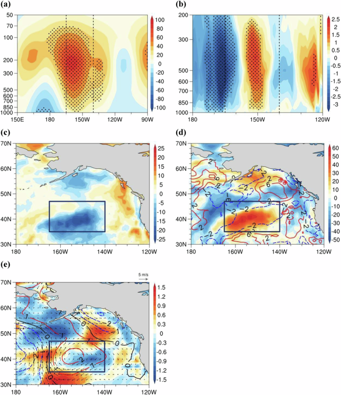
a Longitude-height cross-section of geopotential height anomalies (gpm) in July 2020 along 35°–47°N, in which the stippling area is for the anomaly > 1 std. b Same as in (a), but for vertical velocity ((times)0.01 Pa ({{rm{s}}}^{-1})). c Cloud cover anomalies (%) in July 2020. d Same as in c but for the net surface shortwave radiation (shading; W ({{rm{m}}}^{-2})), the mixed-layer depth (contours; m). e Same as in c but for 10-m wind speed (shading; m ({{rm{s}}}^{-1})), 10-m wind (vector; m ({{rm{s}}}^{-1})), and sea surface pressure (contours; hPa).
Previous research has indicated that there is a potential link between vertical velocity and horizontal flow and that this relationship is related to the climatological thermal structure of the atmosphere30. In the NEP region, isentropic surfaces tilt northwards with altitude in July (Supplementary Fig. 2). Since adiabatic flow moves along isentropic surfaces31,32, anomalous northerly (southerly) flow along the northward tilting isentropic surfaces over the NEP region is conducive to the local anomalous descent (ascent) motion. Because the anomalous northerly wind appears in the eastern part of the high-pressure system in the Northern Hemisphere, the isentropic gliding of the anomalous northerly wind leads to subsidence, suppressing activities of convection and ultimately resulting in decreased cloud cover (Fig. 2b, c). This subsidence extends from the surface to 200 hPa, with the strongest subsidence of 0.02 Pa s−1 around 400 hPa, exceeding one std in the central region of NEP, and results in the reduced total cloud cover in the NEP region. The diminished cloud cover facilitates an increase in the surface net shortwave radiation (Fig. 2d), with anomalous values surpassing 55 W m−2, exceeding one std. Analogously, in July 2020, the increased SWR in the NEP region stemming from a reduction in total cloud cover is consistent with the diagnostic results mentioned above. Concurrently, the high-pressure anomaly within the NEP region dampens surface wind speeds by weakening the climatological mean westerly winds (Fig. 2e). Surface winds are linked to the oceanic mixed-layer depth which signifies the atmospheric influence on oceanic turbulent mixing10. Consequently, the high-pressure anomaly leads to the reduced surface wind speed, and then a shallower mixed-layer depth is observed (Fig. 2d). The depth (11.30 m) diminishes by more than one std, with an anomalous value of −2.38 m. Owing to the augmented net shortwave radiation and the decreased mixed-layer depth, the mixed-layer temperature substantially rises. Notably, the reduced cloud cover, the elevated net shortwave radiation, and the decreased mixed-layer depth in the NEP region coincide with the local occurrence of the MHW event.
The above analyses reveal that corresponding to the high-pressure anomaly in the NEP region, the decrease in cloud cover may result in the increased shortwave radiation and that the reduction in surface wind speed may lead to a decrease in the mixed-layer depth. Collectively, these factors culminate in a notable elevation of the mixed-layer temperature. In the subsequent section, we shall further investigate the possible reason responsible for the formation of the high-pressure anomaly in the NEP region.
Relationship between the warming TP and the MHW event
In the Northern Hemisphere, the high-pressure anomaly is characterized by south and north winds to the left and right sides, respectively. Consequently, we examine the anomalous meridional wind at 200 hPa in July 2020 (Fig. 3a). The observational data clearly reveal the presence of south and north wind anomalies on both sides of the high-pressure anomaly in the NEP region, with their absolute values exceeding 5 m s−1. Concurrently, a meridional wind wave train is observed between the TP and the NEP region. A jet stream may act as the waveguide of Rossby waves33. In Fig. 3a, positive and negative meridional wind anomaly centers of the stationary Rossby wave train are generally located along the extratropical jet stream. The positive anomalies appear in the central-western TP, the Sea of Japan, and the central Pacific Ocean around 170°W; and the negative anomalies appear in East Asia, the central Pacific Ocean around 170°E, and the NEP region. The positive anomalies in the TP and the negative anomalies in East Asia indicate an anticyclonic anomaly between TP and East Asia. An anomalous intense SAH is observed in the TP (Fig. 3b). The geopotential height anomaly extends from the surface to 70 hPa, with the maximum value above 50 gpm around 150 hPa (exceeding one std).
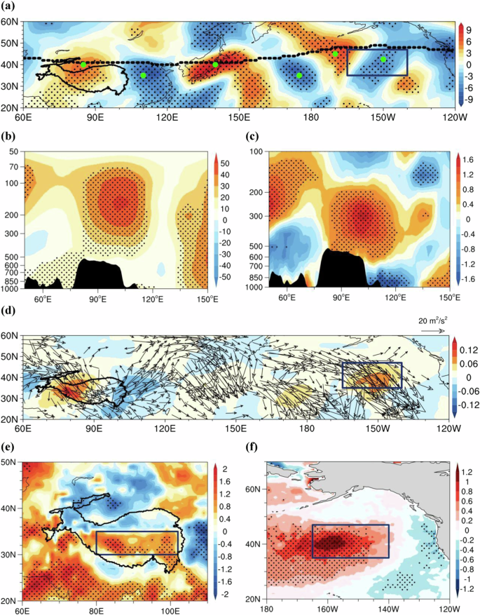
a Meridional wind anomaly (m ({{rm{s}}}^{-1})) at 200 hPa in July 2020. The dashed black line delineates the climatological jet stream axis. Green dots indicate the points (40°N, 85°E), (35°N, 110°E), (40°N, 140°E), (35°N, 175°E), (45°N, 170°W), (42.5°N,150°W) used to define the eigenvalue to represent the wave train. b Same as in a but for the longitude-height cross-section of geopotential height anomalies (gpm) along 31°N. c Same as in b but for temperature anomalies (°C). d 500–200 hPa mean ({{rm{F}}}_{{rm{h}}}) (vector; ({{rm{m}}}^{2},{{rm{s}}}^{-2})) and ({{rm{F}}}_{{rm{z}}}) (shading; ({{rm{m}}}^{2},{{rm{s}}}^{-2})) of anomalous wave. e 2-m temperature anomalies (°C), in which the box is for the area to calculate the thermal condition in the TP (80°E–102°E,30°N–35°N). In a, d, and e the black solid line represents the topography and in (a–c) and (e) the stippling is for the anomaly > 1 std. f Regression of SST (°C) on the thermal condition in the TP in July from 1982 to 2023. Dotted areas represent statistical significance at the 95% confidence level.
Previous research has emphasized that an enhanced SAH can affect the atmospheric circulation in the North Pacific by triggering wave trains from the TP to the North Pacific23,25,26,27,28. We compute the 200–500 hPa mean wave activity flux for July 2020 (Fig. 3d). It is evident that the large horizontal component of wave activity flux (({{rm{F}}}_{{rm{h}}})) emanates from the TP towards the NEP region where the high-pressure anomaly is situated. Concurrently, there are noticeable positive values of the vertical component of wave activity flux (({{rm{F}}}_{{rm{z}}})) in the TP, which might indicate an upward wave activity flux. Within the context of wave activity dynamics, the thermal forcing may be a pivotal contributor to the generation of wave activities34. Therefore, the upward wave activity flux may result from the thermal forcing of the TP. In July 2020, a marked increase in the tropospheric temperature was observed over the TP, with the positive temperature anomaly extending from the TP surface to 200 hPa, with its central value surpassing 1.6 °C and one std near 300 hPa (Fig. 3c). The positive temperature anomalies are also discernible on the surface of TP, with the central value exceeding 1.6 °C and one std in the southern TP (Fig. 3e). The positive surface temperature anomalies coincide generally with the upward wave activity flux.
To examine the robustness of this link between the NEP SST and the TP temperature, we performed a regression analysis between the TP surface air temperature and SST during 1982-2023. Here, the regional mean surface air temperature in the TP (box in Fig. 3e; 80°E–102°E/30°N–35°N) is used to represent the thermal condition in the TP. Figure 3f indicates that the regressed SST in the NEP region closely matches the observation in July 2020. This result shows a significant connection between the NEP SST and the TP temperature. Furthermore, we defined an eigenvalue of the wave train as the algebraic sum of 200 hPa meridional wind anomalies at six specified centers along the wave train that are marked in green in Fig. 3a, that is, V(40°N, 85°E) − V(35°N, 110°E) + V(40°N, 140°E) − V(35°N, 175°E) + V(45°N, 170°W) − V(42.5°N,150°W). The wave train was also found to exhibit significant correlations with both temperatures in the TP and SST in the NEP region, with correlation coefficients of r = 0.32 (p < 0.05) and r = 0.32 (p < 0.05), respectively. This confirms the close link among them. In addition, we also explored the interdecadal relationships among these variables. The interdecadal variability of the TP temperature shows a strong correlation with the interdecadal variability of SST in the NEP region (r = 0.91, p < 0.05). Similarly, the wave train also shows strong correlations with both the temperature in the TP and SST in the NEP region, with correlation coefficients of r = 0.73 (p < 0.05) and r = 0.65 (p < 0.05), respectively. The above analysis suggests that the observed relationships between the TP temperature, the NEP SST, and the wave train are mainly attributed to the contribution of their interdecadal components. Then, are these relationships initiated by the TP heating change?
Some studies have shown that the thermal forcing of TP significantly influences the TP temperature and SAH24,25,28,35,36. Hence, we hypothesize that the wave train from the TP to the NEP region shown in Fig. 3a is a consequence of the TP heating change which culminates in the anomalous intense SAH. To validate this hypothesis, we conduct a diabatic heating forcing experiment using the LBM model. Referring to the observed surface temperature anomalies in the southern TP, the warming TP has an idealized elliptic distribution centered at 87.5°E, 32.5°N (Fig. 4a), an ideal vertical profile with a maximum heating rate of 4 K/day at the surface (Fig. 4b), and a thermal forcing is added over the region (80°E–95°E, 30°N–35°N). This may mimic the direct surface thermal forcing of TP.
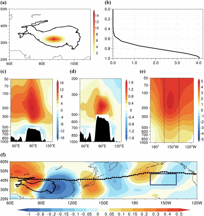
a Horizontal distribution of the ideal diabatic heating (K ({{rm{day}}}^{-1})) used in the LBM model. b The ideal diabatic heating profile (K ({{rm{day}}}^{-1})). c The longitude-height cross-section of geopotential height anomalies (gpm) forced by the TP heating change along 31°N. d Same as in c but for temperature (°C). e Same as in c but for geopotential height anomalies along 35°–47°N. f Same as in c but for the horizontal distribution of 200 hPa meridional wind anomalies (m ({{rm{s}}}^{-1})). The dashed black line delineates the climatological jet stream axis.
Figure 4c shows the longitude-height cross-section of the simulated geopotential height anomalies. It is seen from this figure that positive anomalies predominate over TP and extend upward from 500 to 50 hPa, which indicates a strengthened SAH. Figure 4d shows the longitude-height cross-section of the simulated temperature anomalies. In this figure, positive temperature anomalies appear over TP from the surface to 200 hPa, which indicates a warmer troposphere. These simulated anomalies in geopotential height and temperature are similar to the observations. This implies that the observed anomalies over TP can be forced by the TP surface heating change. Concurrently, a wave train of the 200 hPa meridional wind extends from the TP to the NEP region, with the positive centers in the central-western TP, the Sea of Japan, and the central Pacific Ocean around 170°W and the negative centers in the eastern TP and East Asia, the western Pacific Ocean around 160°E, and the NEP region (Fig. 4f). Corresponding to the positive and negative centers around the NEP region, a deep high-pressure anomaly dominates over the NEP region, with the maximum value in the upper troposphere (Fig. 4e). The simulated features in the wave train from the TP to the North Pacific and the anomalous high-pressure in the NEP region are generally similar to the observations. The similarity demonstrates that the observed atmospheric circulation anomalies from the TP to the NEP region can result from the TP surface heating change.
Since the LBM model is an idealized atmospheric linear model, we further conducted the simulation experiments using the CESM1. Two sensitivity experiments (CESM-Tree and the CESM-Soil) are designed by modifying the surface conditions on the TP. This artificial modification can cause a change in albedo, resulting in local surface heating change and temperature increase, which mimics a TP heating scenario24,28,37. Relative to the CESM-Soil (a higher TP surface albedo), the CESM-Tree (a lower TP surface albedo) forces an increased surface temperature in the TP area (Fig. 5a). Similar to the observations, a wave train of the 200 hPa meridional wind extends from the TP to the NEP region, with the positive centers in the TP, the Sea of Japan, and the central Pacific Ocean around 170°W and the negative centers in the East Asia, the central Pacific Ocean around 170°E, and the NEP region (Fig. 5c), and there is a high-pressure anomaly in the NEP region (Fig. 5c). The similarity between observation and model suggests that the observed atmospheric circulation anomalies from the TP to the NEP region may be attributed to the TP heating change. The high-pressure anomaly in the NEP region has also resulted in a rise of the local SST (Fig. 5b). Compared to the observations, the location of the modeled SST anomaly exhibits a southwestern shift, which is likely due to the gradual southwestward tilt of the modeled NEP high-pressure anomaly from the upper troposphere to the lower troposphere (Supplementary Fig. 3). Nevertheless, the model still captures the primary characteristics of the observational atmospheric circulation changes and the impact of atmospheric anomalies on the NEP SST. Therefore, the unprecedented MHW event in July 2020 and the associated atmospheric conditions could be physically generated by the TP heating change.
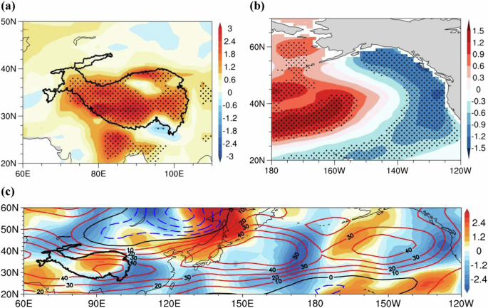
a Composite differences in 2-m temperature anomalies (°C) in July between the CESM-Tree and CESM-Soil. Dotted areas represent statistical significance at the 95% confidence level. b Same as in a but for SST anomalies (°C). c Same as in a but for meridional wind anomalies (shading; m ({{rm{s}}}^{-1})) and geopotential height anomalies (contours; gpm) at 200 hPa.
Discussion
This research analyzes the features of an exceptionally intense MHW event occurring in the NEP region during July 2020, the associated influential factors, and the physical mechanisms of the TP thermodynamic influence on this MHW event through statistical methods, physical diagnosis, and numerical simulation. The results show that the NEP region is besieged by persistent and intense SSTA in July 2020, with the maximum SSTA > 4 °C, the most severe event since 1982. The dynamic and thermodynamic diagnoses exhibit that the local net surface heat flux anomaly associated with the increased SWR is the primary driver of the increased SST, while the oceanic processes likely play a minor role.
The intense SWR may be a direct consequence of the tropospheric high-pressure anomaly in the NEP region. The high-pressure anomaly is accompanied by anomalous subsidence motion at its eastern flank, which leads to a decrease in cloud cover. The reduction in cloud cover further intensifies the SWR reaching the oceanic surface. Concurrently, this high-pressure anomaly also causes a decrease in surface wind speed, which might result in a shallower mixed-layer depth. Therefore, the increased SWR and the decreased mixed-layer depth associated with the high-pressure anomaly over the NEP region contribute to the occurrence of the local MHW event.
Associated with the high-pressure anomaly in the NEP region in the 2020 MHW event is a large-scale wave train over the extratropical sector from Asia to the North Pacific, with the large wave activity flux vectors stretching from the TP to the NEP region. Corresponding to such a wave train, there is a warming TP from the surface to the troposphere and there is an intensified SAH. The simulation results demonstrate that the TP heating change can trigger the local surface and tropospheric warming, enhance the SAH, and facilitate a wave train from Asia to the North Pacific, with a stable high-pressure anomaly and an increase in SST over the NEP region. Since the geopotential height is proportional to temperature, the former may exhibit a rapid increase due to the thermal expansion of air, especially in the upper troposphere38. This phenomenon possibly leads to an overestimation of the strength of geopotential height. Thus we also analyzed the features of geopotential height after removing its trend and obtained the same conclusion.
This study offers new insights into the physical mechanisms connecting the MHW events in the extratropical North Pacific with the climate dynamics of the TP. A lot of studies have revealed that in future climate scenarios, the TP is projected to undergo a sustained warming trend39. In accordance with our finding, the persistent warming of the TP under the future scenarios is expected to contribute to the formation of high-pressure anomalies over the extratropical North Pacific and the occurrence of local MHW events. This heightens the risk of escalating MHW events in these areas in future scenarios.
Some studies showed that precipitation along the Yangtze River basin in the summer of 2020 could release lots of condensation latent heat40,41. To investigate the possible effect of the condensation latent heat in the Yangtze River basin on the wave train associated with the NEP SST, we examine the link between the condensation latent heat (Q2) and the NEP SST. The result shows that there is no significant correlation (r = −0.15, p > 0.1) between the NEP SST and the condensation latent heat in the Yangtze River basin during 1982–2023. The LBM experiment also exhibits that the positive and negative centers of the Rossby wave train forced by the latent heat anomaly in the Yangtze River basin (Supplementary Fig. 4) show a remarkable shift over East Asia (Supplementary Fig. 4d) compared to the observation (Fig. 3a). This difference in the source region indicates that the atmospheric latent heat in the Yangtze River basin might be not a primary factor for the Rossby wave train and the MHW event in the NEP. Furthermore, it is crucial to acknowledge that the occurrence of an extreme event is often the culmination of multiple interacting factors. For instance, the abrupt reduction in global SO2 emissions during the COVID-19 pandemic in 2020 could have weakened the aerosol cooling effect, leading to short-term warming42. Additionally, the substantial reduction in contrails during this period43, which normally reduces infrared radiation emitted back into space, may have increased surface downward shortwave radiation and, consequently, SST. These aspects and their relationship with the MHW necessitate further investigation.
Methods
Data sources
In this study, the monthly and daily mean sea surface temperature (SST) data come from the National Oceanic and Atmospheric Administration (NOAA) optimum interpolation SST version 2 (OISST.v2)44,45. The three-dimensional monthly oceanic temperature, current, and mixed-layer depth data are from the National Centers for Environmental Prediction (NCEP) Global Ocean Data Assimilation System (GODAS)46. The atmospheric variables, including geopotential height, wind, air temperature, surface latent/sensible heat flux, surface net shortwave and longwave radiations, specific humidity, and total cloud cover, come from the monthly and daily data of the European Center for Medium-Range Weather Forecasts Reanalysis v5 (ERA5)47. All datasets cover the period 1982–2023. To examine the robustness of the results, we also used the BOA_Argo mixed-layer depth data from 2004–202348.
Definition of MHWs
Based on the method of Hobday et al.49, an MHW event is defined as SST exceeding the 90th percentile of the baseline climatology for at least five consecutive days, in which a time interval of 2 days or less between two consecutive events is considered as one consecutive event.
Statistical information
The statistical significance of the linear regression, the Pearson correlation and the composite analysis is evaluated with the application of a two-tailed Student’s t-test. We employed the 9-year running average to derive the interdecadal component of one time series. For the interdecadal component, we consider the reduction in degrees of freedom when calculating the significance.
Ocean mixed-layer heat budget
To compare the roles of dynamic and thermodynamic processes in inducing the 2020 NEP MHW, we conduct a monthly analysis of the mixed-layer heat budget. Following previous studies12,50,51, the mixed-layer heat budget equation is written as follows.
Where ({(cdot )}_{a}) indicates the monthly mean anomaly; ∇ denotes the horizontal gradient operator; T denotes the mixed-layer temperature; Qnet denotes the downward net surface heat fluxes including longwave radiation, shortwave radiation, latent heat flux, and sensible heat flux; H is the mixed-layer depth; V (u and v) is the horizontal oceanic current velocity. Additionally, ({{rm{rho }}}_{0}=1015,{rm{kg}},{{rm{m}}}^{-3}) denotes the density of seawater and ({{rm{C}}}_{{rm{p}}}) = 4000 J ({({rm{kg; K}})}^{-1}) is the specific heat of seawater. The above equation is used to explain the mixed-layer temperature anomaly tendency.
Wave activity flux
Wave activity flux (WAF) is a tool for analyzing the activity area of anomalous waves and wave propagation, which may identify the origin of a wave train. We adopt the conventional definition of WAF (({{rm{F}}}_{{rm{s}}})) as outlined below34.
Where (bar{(cdot)}) and ({(cdot )}^{{prime} }) indicates the zonal mean and the zonal deviation; ({rm{varphi }},{rm{lambda }},{rm{Phi }}), ({rm{f}}=2Omega sin {rm{varphi }}), a, and (Omega) denotes the latitude, the longitude, the geopotential, the Coriolis parameter, the radius of the Earth, and the rotation rate of the Earth, respectively. Additionally, ({rm{z}}=-{rm{H}}times mathrm{ln}(frac{{rm{p}}}{{{rm{p}}}_{0}})), H = 8 km is the Scale Height, and ({rm{kappa }}approx 0.286) is the ratio of gas constant to specific heat at constant pressure. The horizontal vector of Fs is defined as Fh and the vertical components of Fs is defined as Fz.
The condensation latent heat
The atmospheric apparent moist sink (Q2) that represents the latent heat due to condensation or evaporation processes and subgrid-scale moisture flux convergences are estimated as follows52,53.
Where L denotes the latent heat of condensation; q denotes the specific humidity; V denotes the horizontal velocity vector; ω denotes the vertical p velocity; p denotes the pressure.
Experimental setup in the LBM
The atmospheric linear baroclinic model (LBM) is widely used to validate the response of atmospheric circulation to diabatic heating/cooling54,55. This model is based on a linearized version of the time-integrated primitive equations6 and can serve as a useful tool for analyzing the influence of anomalous diabatic heating on atmospheric circulation. In this study, we used the LBM to examine whether a prescribed surface heating change over TP can drive a Rossby wave train from the TP to the NEP. The LBM with a nominal horizontal resolution of T42 and 20 vertical sigma levels is run up to 30 days. The variables averaged over the last 10 days are utilized to represent a steady response of the atmosphere to the idealized surface forcing.
Experimental setup in the CESM
We used the Community Earth System Model, version 1.2.1 (CESM1) developed by the NCAR. The CESM1 is a fully coupled global climate model27. We used the f19_g16 configuration with approximately 2.5° horizontal resolution for the atmospheric model and approximately 1° horizontal resolution for the ocean model. Two sensitivity experiments are designed: the CESM-Tree and the CESM-Soil. Referring to previous studies24,26,28, in the CESM-Tree, the surface vegetation type at each grid point in the TP (with the topography > 3000 m) to the south of 35°N is set to the needleleaf evergreen temperate tree, which has a lower surface albedo. The CESM-Soil mirrors the CESM-Tree but replaces the needleleaf evergreen temperate tree with bare soil, which has a higher surface albedo, and in the CESM-Soil, we changed the soil color to the one with the highest surface albedo within the TP to the south of 35°N. In these experiments, the CESM is integrated for 30 years and the outputs from the final 10 years are analyzed.

 region")
Responses