A kinematic analysis of extratropical cyclones, warm conveyor belts and atmospheric rivers

Introduction
The field of atmospheric sciences is rapidly expanding, with an increasing number of scientific publications each year. As emphasis shifts toward viewing the Earth system as a whole, traditional disciplinary boundaries are increasingly overlapping, and similar phenomena are being studied through diverse scientific approaches. Unifying these viewpoints and identifying common concepts, while addressing contradictions or discrepancies, brings significant benefits. It reduces confusion and duplication, enables more focused research, and ultimately enhances our understanding and predictability of the impacts arising from weather systems.
This paper offers a new kinematic framework to unify synoptic-dynamic research for three mid-latitude phenomena, specifically extratropical cyclones (ETCs), warm conveyor belt (WCB) airflows and atmospheric rivers (ARs). ARs are defined synoptically as long, narrow, and transient ribbon-like structures of strong horizontal water vapour transport exceeding a threshold value of vertically integrated water vapour transport (IVT) or total column water vapour (TCWV). ETCs are large-scale cyclonic systems that form outside the tropics. An excellent review of the extensive literature concerning them can be found in1. Briefly, they are characterized by a low-pressure centre and fronts, regions of sharp atmospheric temperature (and moisture) gradients. Associated with these fronts are long-lived wind speed maxima that move with the fronts, known as ETC airflows. The narrow stream of air ahead of the cold front is known as a warm conveyor belt (WCB). The WCB structure exists for a significant portion of an ETC’s lifespan, often remaining coherent for several days. It transports warm and moist parcels of air polewards and thus frequently satisfies the criteria of an AR. An individual air parcel’s journey along the WCB is much shorter than the lifetime of the WCB itself. Thus air parcels are transient within the WCB, constantly being replaced as new air enters the WCB.
The evolution of ETCs, WCBs and ARs can be understood from either an Eulerian or a Lagrangian perspective, each providing distinct insights. The Eulerian view focuses on analysing atmospheric fields in a frame of reference fixed relative to the Earth’s surface. The Lagrangian perspective can be divided into fully Lagrangian and quasi-Lagrangian approaches. A fully Lagrangian view focuses on the evolution of trajectories of individual air parcels, so uses a frame of reference fixed relative to the moving air parcels. The quasi-Lagrangian approach is often used to track features such as ETCs and ARs, thus the frame of reference is fixed relative to the moving feature of interest. Despite their differences, Eulerian, quasi-Lagrangian or fully Lagrangian methods provide complementary frameworks for analysing ETCs, WCBs and ARs. Occasionally studies attempt to combine these 3 frameworks to arrive at a complete picture2 but this is not typical
There have been several previous articles discussing the similarities and differences between ETC fronts, WCBs and ARs. These articles usually focus on a comparison of the phenomenological description of these features3. Since ETC fronts, WCBs and ARs are identified using different methodologies, the criteria for all is not often met at the same location and time. This has led to disagreements within the field regarding their relationship and fragmentation of the scientific literature with respect to these features. Rather than focus on their physical description, we choose instead to concentrate on the mechanisms responsible for their formation. In order to illustrate these dynamical mechanisms we use kinematic analysis to create schematic diagrams which synthesise the evolution of these features. Kinematic analysis uses the motion of the atmosphere to describe the physical attributes of evolving features in a simple, intuitive way, while providing direct links to the understanding of the dynamical causes of them. Through this approach, we hope to enhance the cohesion of mid-latitude synoptic-dynamic meteorology, bridging gaps, and encouraging a more unified approach to studying mid-latitude atmospheric phenomena.
Kinematic analysis
Meteorologists often choose between categorising phenomena based on their physical attributes or the underlying physical laws. Synoptic meteorology is largely based upon their physical attributes and historically has involved the meticulous analysis of large-scale charts representing surface and upper-level patterns of pressure, wind, temperature, and humidity. These analyses were performed by meteorologists using ground-based4 and upper-air5 measurements. Dynamical meteorology applies physical laws to explain atmospheric motions and energy transformations6,7 underlying weather phenomena. Dynamical theories are derived from the governing equations with a hierarchy of intermediate approximations depending on the scales of motion being investigated. These simplified equations provide the basic dynamics necessary to understand the mechanisms responsible for the formation of ETC airflows and ARs. A third combined approach analyses diagnostics from Numerical Weather Prediction (NWP) analysis and reanalysis datasets. These datasets have largely replaced manual synoptic analysis and have the advantage that they provide long time-series of dynamically consistent 3-dimensional data. The language and tools of these varied approaches are different, leading to some difficulties comparing and contrasting results from different studies.
One way to bridge the gap between the synoptic analysis of ETC, WCB and AR structures and a dynamical analysis of the forces responsible for their formation, is to study the atmospheric motion without regard to forces that cause it. This is known as kinematic analysis. Kinematic analysis is a simpler method than dynamic analysis and is particularly useful for motion with no rapid accelerations. In this paper kinematic analysis and schematic diagrams will be used to describe the physical evolution of ETCs, WCBs and ARs as they go through their lifecycle.
In the kinematic analysis we shall employ, the motion and change in shape of any parcel of air in the atmosphere over a time δt can be decomposed into individual components of the flow using Taylor expansion. Decomposing the atmospheric flow into the mean flow (translation) and components that involve derivatives of the flow (rotation, convergence and strain) allows us to study and understand the underlying mechanisms influencing atmospheric dynamics more easily. The effect of different components of the flow listed below are shown schematically in Fig. 1.
-
Translation: The uniform movement of air parcels from their origin by the mean flow. Translation describes how moisture is transported within an AR if it is not removed from the atmosphere through precipitation.
-
Rotation: The clockwise or anticlockwise rotation of air parcels about the origin is measured by vorticity. How vorticity changes with latitude helps us understand the evolution of large-scale atmospheric waves.
-
Convergence: The expansion or contraction of air parcels due to horizontally divergent or convergent flow. When air converges horizontally at the surface, upward motion must occur above due to the quasi-incompressibility of the atmosphere. Similarly, when air diverges horizontally at upper-levels, upward movement must occur beneath. Thus convergence and divergence are important for understanding WCB ascent and ETC precipitation.
-
Strain: The changing shape of an air parcel due to stretching flow. Strain influences the development of atmospheric features such as fronts.

These components are, translation, rotation, convergence and strain. (Solid) Shape of fluid parcel at initial time, t0. (Dashed) Shape and position of fluid parcel at later time, t0 + δt, following action of kinematic component of flow. Blue line indicates the axis of dilatation and red line indicates the axis of contraction. Δλ is the horizontal length scale over which rotation, convergence and strain are acting.
Terminology
Given the differences in language used by different scientific communities, here it will be useful for subsequent discussion to clarify some terminology. For further reading we refer the reader to these excellent dynamical meteorology textbooks8,9,10.
The term ETC has two parts – ‘extra-tropical’ and ‘cyclone’. The latter implies roughly circular (vortical or eddy) motion around a centre. The former generally distinguishes the structure of interest from tropical cyclones that have very different scales, structure and mechanism. As discussed by1, a precise definition of extratropical cyclones is difficult, as each is different. Furthermore, a number of mechanisms result in the growth of cyclonic flows. They result from instability of the environment in which they develop, and also help shape that environment.
Before discussing ETCs in more detail, it is important to discuss the environment in which they develop. The atmosphere is a fluid layer, much thinner in vertical extent than horizontal, above the surface of the rotating earth. The angular momentum associated with this planetary rotation, combined with fact that it is usually stable with respect to small vertical perturbations, impacts atmospheric dynamics considerably. The dynamics result in a number of wave motions, the most meteorologically important in the extra-tropics being Rossby waves. These result from meridional variation of the effective earth rotation rate with respect to the earth’s surface. Rossby waves are approximately geostrophically-balanced flows; geostrophic balance means the horizontal Coriolis force, which results from the Earth’s rotation, exactly balances the horizontal pressure gradient force, which arises from differences in air pressure (and hence differences in column mass). Thus, positive and negative perturbations of the pressure field (known as ridges and troughs) are associated with pole-ward (between trough and ridge) and equator-ward (between ridge and trough) perturbations of the horizontal flow.
Geostrophic balance also implies that horizontal temperature gradients are associated with horizontal differences in the change of atmospheric pressure with height, which, in turn, leads to changes in the horizontal geostrophic wind with height. This is known as thermal wind balance since changes in the horizontal thermal gradients are balanced by changes in the geostrophic wind profile. As a result of thermal wind balance the global-scale meridional temperature gradient is associated with the formation of jet-streams near the tropopause.
Rossby waves occur on a wide range of scales in the troposphere and explain many atmospheric features. The largest are known as planetary-scale waves. There are typically between 2 and 6 planetary-scale waves with horizontal wavelengths of 4000-8000 km’s surrounding the Northern and Southern Hemisphere at any given time. They are often most obvious in the form of the meridional meander of the jet-stream due to waves near the tropopause, though planetary-scale troughs and ridges generally extend through a significant depth of the atmosphere, often reaching from the upper to the lower troposphere.
Planetary-scale waves can be quasi-stationary (especially when associated with the land/sea distribution). They can also have such a large amplitude that closed contour high (anti-cyclonic) and low (cyclonic) pressure centres occur that reach the surface; in the latter case they can be termed ETCs. Such large-amplitude planetary-scale troughs are thus identified as large ETCs with positive vorticity (due to the cyclonic curvature of the flow) and with continental-scale cold air masses moving towards the equator (known as cold-air outbreaks) and poleward movement of warm and moist air (constituting a tropical moisture export).
As will be discussed in more detail below, the flow associated with large-scale trough-ridge systems can dynamically promote the generation of smaller, synoptic-scale ETCs (i.e. cyclogenesis) with horizontal wavelengths of 1000 km to several 1000 km, often through interaction of the upper-level flow with near-surface temperature gradients (i.e. baroclinic processes). Furthermore, the trailing cold fronts of a large ETC (known as a primary or parent ETC) can become unstable and multiple ETCs can develop (known as secondary ETCs)11,12. Thus, in general synoptic-scale ETCs are associated with larger-scale low-pressure regions and may propagate into them. Hence it is often difficult to distinguish the two without some form of time and/or spatial filtering.
The boundary between two distinct airmasses is known as an atmospheric front. The leading edge of cold air outbreaks is thus a cold front forming a boundary between cold polar air moving equator-ward and warmer (and moister) tropical air moving pole-ward (both generally also with a zonal component). The vertical wind shear associated with the horizontal temperature contrast between the airmasses produces strong along-front quasi-horizontal wind maxima (known as low-level jets). As a result, the associated heat and moisture transports are generally concentrated over a relatively small horizontal extent (of order 100 km). The trailing cold front of a large ETC can extend several thousands of km’s along a planetary-scale trough. The low-level jet on the warm side of a cold front is part of the WCB airstream and the transport of water vapour by this low-level jet is labelled an AR. Thus frequently WCBs and ARs are identified ahead of these elongated cold fronts with very large horizontal and meridional extent. This was illustrated by the tracer transport study of13 who showed that ARs were composed of a sequence of meridional excursions of water vapour, in close correspondence with the upper-level wave pattern.
Waves in the atmosphere are not moved by the flow they are embedded in, but instead propagate relative to it, i.e. they may move faster or slower than or in a different direction to the ambient flow. This is important as the movement of ETCs is determined by the wavelength-dependent propagation speed of these waves (known as their phase velocity). Thus air constantly enters and exits waves and the features associated with them, such as WCBs and ARs. As a result, the evolution of WCBs and ARs are contingent upon the trajectories and properties of the air parcels entering and leaving them.
Mid-latitude feature Identification
Several methods (and hence, definitions) are used to identify ETCs, WCBs and ARs in the atmosphere. Regardless of whether Eulerian, Lagrangian or quasi-Lagrangian approaches are used, most methods employ some form of conditional sampling, i.e. utilising only part of a dataset that satisfies certain criteria associated with the coherent structures of interest. In the context of synoptic-dynamic meteorology, conditional sampling has particularly been used to identify features in the atmosphere that persist over several days. Two common conditional sampling methods are (i) spectral analysis and (ii) feature tracking. In the context of this paper, spectral analysis is a mathematical method used to study the dynamics and energy transfer of synoptic waves in the atmosphere whereas feature tracking is a method used to monitor and track the physical attributes of synoptic-scale features. Eulerian spectral analysis and quasi-Lagrangian feature tracking methods can also be combined, as we describe in the Methodology section.
Spectral analysis is more frequently used in studies that apply dynamical analysis to study ETCs and ARs. First flow decomposition (often referred to as Reynolds decomposition) is applied to timeseries information at a point. This involves decomposing the atmospheric flow into two main components: the mean flow (background) and perturbations to the mean flow (turbulence). Let ϕ be a scalar quantity (e.g., water vapour, temperature or mass) in the atmosphere. The turbulent flux of ϕ in the direction of the velocity component u can be mathematically expressed as the product of the turbulent velocity ((u^{prime})) and perturbation quantity ((phi ^{prime})), such that
(Here, the term ‘turbulent’ is used in the broad sense as the part of the flow that fluctuates from the mean (represented by the overbar), and does not imply any particular form of dynamical instability or time-scale of the fluctuations.)
The method of conditional sampling focuses on the structures that contribute to turbulent fluxes since the mean flux is constant in time. In order to consider the coherence of features such as ETCs and ARs in time, it is common to partition the turbulent flux into different frequency classes using spectral analysis. Certain coherent structures exhibit distinct frequency characteristics. For example, applying a 2-8 day bandpass filter will filter out tropospheric waves in the atmospheric data with frequencies above and below these limits (such as quasi-stationary planetary-scale troughs and mesoscale circulations). The remaining waves are typically associated with synoptic-scale transient features, such as ETCs and ARs.
This approach has been used in both the AR and ETC literature. For example, Fig. 2a, from14, shows results for the global ETC storm tracks obtained by applying a high bandpass filter (10 days) to the eddy kinetic energy field, (frac{1}{2}(overline{{u}^{{prime}{2}}}+overline{{v}^{{prime}{2}}})), (coloured shading). The filtered field shows the synoptic-scale waves and we can clearly identify the ETC storm tracks in the North Atlantic, North Pacific and Southern ocean basins as regions of high amplitude synoptic-scale variability. The earliest identification of ARs also applied spectral analysis to the study of moisture fluxes in newly-available reanalysis data. For example,15 found that meridional moisture fluxes, (overline{{v}^{prime} {q}^{prime}}), are concentrated in filamentary structures and that much of the total flux was carried by the mean properties of these structures.16 apply band-pass time filters (shorter than 3 days, 3–6 days, and longer than 6 days) to the moisture flux atmospheric data to identify 3 different classes. Figure 2b shows the amplitude of variability of the filtered moisture flux field they derive using the 3-day high-pass filter for January 1992. Again, there are maxima in the North Pacific, North Atlantic and Southern Oceans which are identified regions of strong AR activity. In an analogous manner, both horizontal heat and moisture fluxes (typically described as (overline{{v}^{prime} {theta_{w}}^ {prime}}), where θw is the wet-bulb potential temperature), and vertical heat and moisture fluxes ((overline{{omega}^ {prime} {theta_{w}}^ {prime}})), in the vicinity of ETCs or along Lagrangian trajectories, can be used to identify WCBs since WCBs are characterised by strong horizontal and vertical transport of warm air.
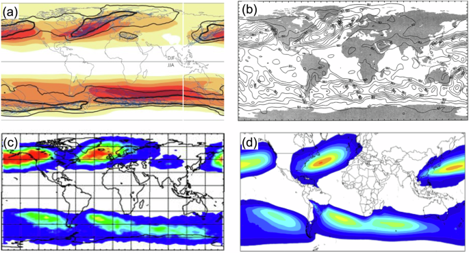
a Climatology of wintertime ETC track density (black contours) and 10-day high-pass filtered Eddy Kinetic Energy (coloured shading) adapted from from14 (their figure 1), b Amplitude of high frequency filtered water vapour flux for January 1992 from16, c Climatology of wintertime WCB frequency adapted from from23 and d Climatology of AR frequency from19. Figures have been centred on 0∘ longitude and, where possible, winter hemispheres are shown. Colourbars have been deliberately removed to focus on patterns of high feature frequency rather than magnitudes which depend on individual criteria used to identify features.
Rather than analyse the synoptic-scale wave activity at fixed geographical locations, it is also possible to develop criteria with which to identify and track the movement of features associated with tropospheric waves (i.e. ETCs, WCBs and ARs). Feature tracking refers to the identification of coherent structures based on a synoptic understanding of their spatio-temporal characteristics. Conditional sampling is used to identify features within datasets according to a set of criteria, which are then labelled and tracked in space and time. Thus feature tracking enables the extraction of relevant information from a dataset in quasi-Lagrangian or Lagrangian frameworks.
From the AR literature,17 proposed that the vertical integral of the moisture flux (IVT) could be used to identify ARs. They proposed an objective method for identifying ARs using a latitudinally varying IVT threshold criteria, such that:
The value 0.3 is empirical and gave the best preservation of AR structure on the day chosen. Many AR identification algorithms also include criteria specifying the spatial structure of ARs, for example18 recommend using criteria to specify IVT direction (coherent and directed along the shape elongation, with a mean poleward component exceeding 50 kg m−1 s−1), length (>2000km), and length/width ratio (>2). A recent AR climatology has been produced by19 and shown in fig. 2(d). Despite using a different method for performing the conditional sampling of ARs, regions of maximum frequency of occurrence are found in the same location as those with highest synoptic-scale moisture flux variability. While these criteria identify ARs as an Eulerian concept, recognising that AR structures exist (albeit with some movement or change of shape) for a significantly longer time than it takes air to move through the structure, allows ARs to be identified in space and tracked over time. In this quasi-Lagrangian framework it is therefore possible to evaluate the lifecycle of an AR and flow relative to the motion of an AR20.
ETCs are part of propagating wave patterns but they can also be identified as coherent Eulerian features in space using methods that identify minima in mean sea level pressure or geopotential height, positive relative vorticity maxima or coherent cloud and precipitation patterns. Additional characteristics of ETCs are often used to ensure that the identified features are of sufficient strength, duration and mobility. For example,21 recommend using criteria to specify minimum intensity (relative vorticity > 5 × 10⁻⁵s−1), lifetime (≥ 48 hours) and track length (> 1000km). There is significant overlap between the regions of high ETC activity identified using the spectral analysis method (coloured contours) and the feature tracking method (black contours) in Fig. 2a demonstrating that the dynamical and synoptic methods produce similar results.
Like ARs, WCBs are coherent airflows which evolve but retain their structure while air parcels move along them, hence the concept of a ‘conveyor belt’. They can be identified using quasi-Lagrangian or Lagrangian methods. Following the work of22, it was recognised that (dry) airflows are approximately isentropic, i.e. in the absence of turbulent mixing and radiation, they conserve their entropy and hence potential temperature as they ascend or descend in the atmosphere. Thus streamlines (lines tangential to the direction of the instantaneous wind vectors at each point) on isentropic surfaces in the frame of reference of moving ETCs are often used to identify coherent 3D ETC-relative airflows in a quasi-Lagrangian framework. Since isentropic surfaces slope upwards from warmer regions to cooler regions, poleward ETC-relative movement is broadly associated with ascending airflows while equatorward ETC-relative movement behind ETC cold front is associated with descending air flows. Typically WCB air flows are identified on relatively warm potential temperature surfaces which are typically quasi-horizontal and close to the surface in the warm sector of ETCs, but then slope upwards above the cold and warm-frontal zones. When sufficient ascent occurs for cloud to form a moist potential temperature surface (wet-bulb or equivalent) is more appropriate but the same result applies.
An alternative fully Lagrangian method of identifying WCBs and ARs is to compute the path of air parcels, or trajectories. Coherent ensembles of trajectories can be found the details of which depend upon criteria used to conditionally sample the trajectories. Thus it is unlikely that a one to one correspondence between the quasi-Lagrangian and Lagrangian WCB and AR structures will emerge. Nevertheless, closely-related structures do emerge.23 identified WCB if, during the first 2 days, trajectories travelled more than 10∘ longitude to the east and more than 5∘ latitude to the North, and ascended by more than 60% of the zonally and climatologically averaged tropopause height at the trajectory’s latitudinal position after 2 days. Figure 2c shows a climatology of wintertime WCB frequency. As for the ETC and AR climatologies, regions of maximum WCB activity are found in the ocean basins.
In summary, both dynamical and synoptic analysis methods in Eulerian, quasi-Lagrangian or Lagrangian frameworks can be used to identify and analyse ETCs, WCBs and ARs. Given the different methods and definitions used they are unlikely to perfectly coincide, but broadly speaking the climatological frequency patterns and inter-seasonal variability (not shown) are consistent. It is not the aim of this paper to compare and contrast these methods, but to focus instead on providing a synthesis of the concepts regardless of the different methods, definitions and terminology used in their individual analysis.
The structure of the paper is as follows. The results section provides a synthesis of the literature on cyclogenesis and tropical moisture exports; frontogenesis, WCB and AR development; and finally diabatic heating, secondary cyclogenesis, ETC and AR families. Each of these sections starts with a synoptic explanation of the topic, followed by a dynamical description and ends with a kinematic synthesis providing a bridge between the synoptic and dynamic descriptions. In the Discussion section, we discuss some common myths in the literature that have arisen as a result of difficulties comparing and contrasting results from different synoptic and dynamical studies. These myths relate to the distinctness of WCBs and ARs, the subtropical source of precipitation in ETCs, and the role of ARs in secondary cyclogenesis. In the Methodology section we introduce the kinematic analysis method we use.
Results
Cyclogenesis and tropical moisture exports
In this section, we consider the earliest stages of ETC formation (known as cyclogenesis) and AR formation (known as a tropical moisture export). We start with a synoptic description of this early stage in the evolution of an AR, followed by a dynamical description and end with a kinematic synthesis providing a bridge between the synoptic and dynamic descriptions. We use the kinematic synthesis to build a schematic diagram which illustrates the early stages in the lifecycle of an AR (tropical moisture export) and the kinematic components of the flow responsible for it’s formation.
Synoptic description of cyclogenesis and tropical moisture exports
As described in the Introduction, planetary-scale waves appear as successive high and low centres in geopotential height or pressure fields, associated with approximately geostrophically-balanced flows in between. In practical terms, this balance leads to the wind flowing parallel to the isobars in the atmosphere, resulting in typically alternating relatively narrow poleward and equatorward flows. These low-amplitude planetary-scale waves contribute to the largest-scales of meridional moisture and temperature fluxes, drawing out filaments of warm and moist air from the tropics in the ridge part of the wave, and extruding cold and dry air from the polar regions in the trough part of the wave. Even barotropic waves (where density is a function of pressure only) naturally draw out filaments from the regions at their extrema including low-level warm and moist filaments from the subtropics.
The start of ETC development (cyclogenesis) or AR formation (tropical moisture exports) thus begins as a poleward bulge in the water vapour or temperature fields. A ridge in the water vapour field is often referred to as a moist tongue or moist axis in the AR literature. Correspondingly, a ridge in the temperature field is referred to as a warm tongue in the ETC literature24. This difference reflects the different focus on moisture in the AR literature and temperature in the ETC literature (or more specifically potential temperature, which accounts for changes in temperature due to pressure changes, which are common in the atmosphere). The relationship between warm tongues and ARs was discussed by25. Naturally, the definitions of warm tongues and tropical moisture exports/ARs differ, so the intersection of the two sets is not complete. Nevertheless, the conclusion is that the majority of warm tongues would be associated with tropical moisture exports/ARs and vice versa.
The amplitude of upper-level planetary-scale waves can intensify when an eastward-progressing synoptic-scale wave at upper-levels becomes superimposed over a region of strong horizontal temperature gradient associated with a frontal zone at the surface. In this environment, atmospheric density is a function of both pressure and temperature. This is known as a baroclinic environment, where baroclinicity is the horizontal temperature gradient divided by the static stability. When the upper-level wave enters this baroclinic environment the potential energy stored in the atmosphere can be converted into kinetic energy through a process known as baroclinic instability26. Thus, the interaction of a wave at upper-levels and the low-level temperature gradient can lead to the formation and growth of an ETC with strong winds and enhanced moisture transport in an AR.
Dynamic description of of cyclogenesis and tropical moisture exports
In order to explain the physical process of baroclinic instability it is common to assume that the atmosphere is in approximate geostrophic balance, thus neglecting higher frequency wave motions (such as inertia-gravity waves) from the equations of motion. These ‘quasi-geostrophic’ equations enable us to understand the physical processes that effect midlatitude, synoptic features (even though we use a more sophisticated set of equations in NWP because they are more accurate).
Early studies by26 and27 developed dry idealised models of baroclinic instability in a continuously stratified atmosphere which solve the quasi-geostrophic equations. Their initial model state consisted of a meridional temperature gradient (baroclinic environment), vertical wind shear and constant Coriolis parameter. They found that finite amplitude waves can grow from small perturbations to the initial state demonstrating that sharp frontal gradients are not a necessary condition for cyclogenesis. They also showed that the fastest growing baroclinic development was the result of the vertical interaction of phase locked upper and lower level waves with the upper-level wave located upstream of the low-level wave. Weak cold and warm fronts occurred as part of the cyclogenesis process as well as horizontal WCB flow parallel to the surface cold front and ascending WCB flow above the frontal zones (though the term WCB was not used).
This ‘phase-locking’ phenomenon can be explained by a simplified model that analyses the effects of horizontal temperature gradients by considering the atmosphere as two homogeneous layers representing the lower and upper troposphere. A horizontal temperature gradient causes a vertical slope in the isentropic surfaces between the layers, resulting in different pressure gradients and thus varying mean wind speeds in each layer. A key characteristic of atmospheric waves is that their propagation speed depends on their wavelength. In conditions of vertical wind shear28,29, waves of the same wavelength can move at different speeds relative to the flow in their respective layers, but at the same speed relative to each other. This steady phase difference between the waves allows the flow of one wave to enhance the growth of the other, and vice versa, leading to unstable growth.
While we can infer that the strong winds associated with increasing pressure gradients during cyclogenesis in these quasi-geostrophic models would necessarily lead to enhanced moisture transport, the models produced by26 and27 did not contain moisture. Recently30 performed simulations using a moist (single phase) quasi-geostrophic model. They showed that ‘AR-like’ structures could form, provided a meridional moisture gradient and appropriate precipitation rates were prescribed. However, the ARs produced are less sharp than in nature, consistent with the weak frontal structures produced in the dry models. Furthermore, they do not have an elongated meridional extent as observed in the real atmosphere. Thus quasi-geostrophic theory can explain some aspects of ETC and AR cyclogenesis, but not the whole picture.
Kinematic description of cyclogenesis and tropical moisture exports
In this section, we use kinematic analysis to develop schematic diagrams which illustrate cyclogenesis and tropical moisture export formation. The purpose is to provide a bridge between the synoptic warm/moist subtropical extrusion description in the Synoptic description of cyclogenesis and tropical moisture exports section and the dynamical geostrophic theory description of cyclogenesis and subtropical moisture export described in the Dynamic description of of cyclogenesis and tropical moisture exports section.
Figure 3a shows an idealised background state similar to that used in the26 and27 models. It consists of uniform vertical wind shear and a meridional temperature gradient (not shown), additionally we show a meridional moisture gradient. In this idealised setup, the wind is parallel to the isobars and the moisture is simply advected from left to right by the mean background flow, as visualised by the change in position of the example deformation square.
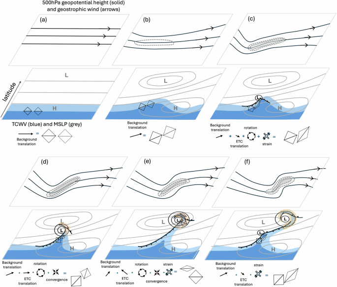
a Idealised initial background state with meridional gradient of total column water vapour (TCWV) (blue shading), mean sea level pressure (grey), 500hPa geopotential height (black) and geostrophic wind (arrows). b Formation of a tropical moisture export (TME) due to advection of moist air around large-scale quasi-stationary surface high pressure centre downstream of planetary-scale trough (black) and associated jet streak (dashed). c Evolution of TME into an AR due to strain flow increasing the moisture gradient and advection of moist air away from the subtropics. d Extension of AR filament into mid-latitudes due to convergence of moist air ahead of the cold front. e Formation of midlatitude AR spiral with depleted TCWV due to strong rotation and strain flow and loss of moisture via precipitation. f Formation of second AR (forming an AR family) due to continued strain maintaining the strength of AR filament in the subtropics. The 850hPa flow acting on a fluid parcel at each stage is decomposed into kinematic components of the flow; translation (background and ETC flow), rotation, convergence and strain components. The action of these components on the shape and position of example fluid parcels is shown by the solid and dashed squares. Note that ETC translation refers to the movement of the fluid parcel by the ETC flow. This is different to the velocity of the ETC which is more closely related to the background translation.
In the real atmosphere, we observe, however, that the mean background state in the midlatitudes consists of quasi-permanent high and low-pressure centres at the surface (Fig. 3b). In the north Atlantic these are known as the Azores high and the Icelandic low. In the north Pacific they are known as the north Pacific high and the Aleutian low. At upper-levels there are quasi-permanent planetary-scale waves consisting of a trough in the geopotential height upstream of the surface low, quasi-permanent ridge downstream of the surface low (not shown), and a local maximum in the wind speed in between denoting the position of the climatological jet stream (Fig. 3b) (known as a jet streak). If we consider the action of the background flow on a fluid parcel (solid diamond in Fig. 3b), we find that translation by the background flow will result in the uniform movement of the fluid parcel from its origin with the velocity of the low-level background wind. Thus at a later time, the meridional moisture pattern will have evolved with moisture to the west of the stationary high pressure being advected polewards. Thus, the (geostrophic) advection of moisture around a quasi-stationary high pressure region is consistent with the formation of a tropical moisture export/warm tongue. However, the narrow filamentary structure of an AR is not yet evident. If the flow is in a geostrophic balance, then the streamlines of the flow are approximately parallel to the isobars. Therefore, moist air will circulate around the closed isobars of the high-pressure region and thus return to the subtropics after some time.
Since the quasi-stationary planetary-scale waves described above are unable to explain the extension of moist filaments of air from the subtropics to the extratropics we next consider the transport associated with synoptic-scale wave features embedded within the longer-wavelength features. These synoptic-scale wave features can propagate eastward relative to the planetary-scale waves and are typically associated with transient features such as ETCs and ARs. Thus we consider a transient ETC embedded in the mean background south-westerly flow field (Fig. 3c) and shortwave trough moving through the planetary-scale trough at upper levels. This ETC may have been generated elsewhere, but quasi-geostrophic theory indicates that ETCs typically form in regions downstream of upper-level planetary-scale troughs and to the right of the jet streak’s entrance region. These areas are characterised by upward motion, which creates favourable conditions for the development of new surface ETCs31.
Figure 4a shows composite ETC-centred fields in the early stages of ETC development (48 hours before maximum ETC intensity). At this early stage in the ETC lifecycle, on average ETCs are travelling towards the east (80∘ to north) as shown by the composite ETC propagation vector. The temperature and moisture fields already exhibit a wave like structure, with colder and drier air displaced equatorwards behind the ETC centre, and warmer and moister air displaced polewards ahead of the ETC centre. Note that the cold front in the composite temperature fields extends 20∘ (>2000 km) from the ETC centre. Due to their varying orientation, the cold fronts far from the ETC centres are not always positioned sufficiently similarly to produce a clear signal in the composite, although rotation of the ETCs prior to compositing minimises this limitation.
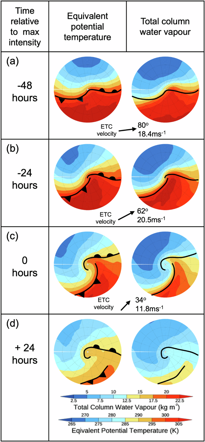
Composite ETC-centred fields (a) 48 hours before maximum intensity, (b) 24 hours before maximum intensity, (c) at maximum intensity and (d) 24 hours after maximum intensity. Column 1: Evolution of 850hPa equivalent potential temperature, overlaid with approximate position of composite cold and warm fronts. Composite ETC propagation speed and direction (vector). Column 2: Total column water vapour.
Composites of the individual components of the 850 hPa flow field are shown in Fig. 5a. On average, the background mean flow acting on a parcel of air located in the ETC warm sector ahead of the cold front (denoted by the solid diamond) advects it in the direction of ETC propagation but at a slower speed. Since the ETC wave moves faster than the flow in which it is embedded, the ETC accelerates away from the parcel of moist air. The geostrophic motion around the ETC (tangential to the isobars) results in the advection of the fluid parcel around the low centre. Cyclonic vorticity (positive rotation) is relatively weak and convergence along the cold front is negligible in the composite at this stage in the ETC lifecycle. Ahead of the ETC’s cold front there is a region of strain, where the anticyclonic flow around the quasi-stationary high pressure meets the cyclonic flow around the transient ETC. This strain flow changes the shape of the fluid parcel, stretching it along the axis of dilatation (parallel to the cold front) and compressing it along the axis of contraction (see Fig. 1) resulting in a strengthening the temperature and moisture gradient across the front (frontogenesis). The combination of these motions results in a translation and deformation of the moisture pattern originally found in the warm sector of a synoptic ETC (Fig. 4a).
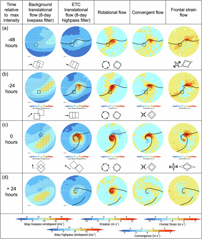
Composite ETC-centred fields a 48 h before maximum intensity, b 24 h before maximum intensity, c at maximum intensity and d 24 h after maximum intensity. Columns 1-5: Kinematic decomposition of the 850hPa flow field into mean translation by background flow (column 1), mean translation by ETC flow (column 2), rotational flow (column 3), convergent flow (column 4) and frontal strain flow (column 5). The action of these flow components on the shape and position of a fluid parcel is shown by the dashed diamond shapes.
Thus, a kinematic analysis of an ETC embedded in a background flow field can describe both the advection of the moisture gradient from the subtropics and its strengthening, creating a more elongated moisture filament than can be produced by the quasi-stationary high and low pressure regions alone. This kinematic analysis 48 hours before maximum ETC intensity is used as the basis for the evolution of the TCWV field in Fig. 3c.
ETCs are not simply moved by the flow they are embedded in, but instead propagate relative to it. In the case of a developing ETC, the ETC moves faster than the flow of water at low-levels, i.e. the component of motion of the ETC from west to east is more rapid than the average westerly component of the wind at the surface which is slowed due to friction. As a result, the moist air in the AR cannot catch up with the ETC which is propagating more quickly into the extratropics so it is effectively left behind by the ETC. Thus use of the term ‘tropical moisture tap’32 to describe the direct long-distance transport of moisture from a tropical source region to the centre of a cyclone is incorrect, since it implies that moisture originating in the subtropics can catch up with the moving ETC centre.
Since moisture filaments are observed to extend from the subtropics to the centre of ETCs there must therefore be an alternative source of moisture available to create the leading end of the AR.13 quantify the fractional contribution of tracers originating in different latitude bands to total precipitation at all latitudes. They find that most of the precipitation in a latitude band comes from that latitude band. For example, in the extratropical North Atlantic (50 − 70∘N),13 find that around two-thirds of the precipitation originates in the extratropics, with the remainder coming from contributions further away and very little of the moisture originates in the tropics (< 30∘N).
To describe the mechanism responsible for extending the AR filament it is necessary to consider the full wind field rather than only the geostrophic wind. This will be described in the next section on ETC frontogenesis and AR development.
ETC frontogenesis and AR development
In this section, we consider the developing stages of ETC formation during which fronts begin to strengthen (known as frontogenesis), WCBs strengthen and produce precipitation, and AR filaments extend into the extratropics. We start with a synoptic description of this stage in the evolution of these features, followed by a dynamical description and end with a kinematic synthesis providing a bridge between the synoptic and dynamic descriptions. We use the kinematic synthesis to extend the schematic diagram illustrating the lifecycle of an AR to include extension of the AR filament into to the extratropics.
Synoptic description of ETC and AR development
Synoptic studies of observational data have produced detailed understanding of ETC frontal structure and evolution. Figure 6a shows a plan view of ETC-relative streamlines (arrows) on an isentropic surface around an ETC located to the north of the Figure33. In the south of the domain moist air ahead of the cold front is flowing at low levels (900 hPa) towards the cold front from the east. As it approaches the cold front this low-level moist airflow (known as the feeder airstream34) splits into two branches with one airflow turning clockwise and ascending parallel to the cold front up to around 700 hPa and forming a band of cloud (dark grey shading) collocated with the cold front. This ascending air flow is part of WCB (as viewed in an ETC-relative framework)35.
Figure 6b shows a vertical cross-section through a sloping cold front from36. ETC-relative streamlines (arrows) show the feeder-airstream approaching the cold front from the environment ahead and the ascending part of the warm conveyor belt rising along the cold frontal surface forming clouds and precipitation as the moist air cools. Note that ascent is above the cold front in this cross-section since36 show a cross-section through a forward-sloping ana-cold front, rather than the more typical backward-sloping kata cold-front. Behind the cold front is shown the descending dry intrusion. There are two jets shown in the schematic, one at upper levels (associated with the planetary-scale jet stream) and another synoptic-scale jet ahead of the cold front, referred to as the pre-cold front low-level jet (LLJ). This pre-front LLJ is the horizontal part of the WCB. It forms due to the acceleration of the wind necessary to maintain geostrophic balance in the along-front direction described in the next section on the Dynamical description of of ETC and AR development. It is clear from36 that the pre-cold front LLJ and ascent are both part of the WCB airflow. This was later expanded on by5 who state that “Following Harrold (1973), we refer to the narrow airstream as the ‘warm conveyor belt, because of its role in conveying large quantities of heat (and also moisture and westerly momentum) poleward and upward”. Figure 6c and d show equivalent plan view and vertical cross-sections to Fig. 6a and b but from an AR perspective37. Here the focus is on horizontal moisture fluxes rather than 3D airflows. The plan view shows an AR co-located with an ETC cold front with high values of TCWV. This elongated filament of high moisture shows remarkable similarity to the cloud filament seen in Fig. 6a. The vertical cross-section through the AR is shown in Fig. 6d. Surprisingly, given the advances in observations, the vertically sloped cold front, cloud and precipitation, upper- and low-level jets are the same as those described by36. The main differences are that the work by36 (Fig. 6b) shows a shallow region of upright convection at the cold front, inferred from radar but likely missed by the dropsondes used in the study by37. Figure 6d also shows the moisture flux (orange shading) at low-levels with a maximum ahead of the cold front. This maximum is a somewhat larger feature than the pre-cold front LLJ, but this is merely a matter of choice of threshold. Thus even though the definitions of an AR and the horizontal part of the WCB differ, it is clear that the structures are the same.
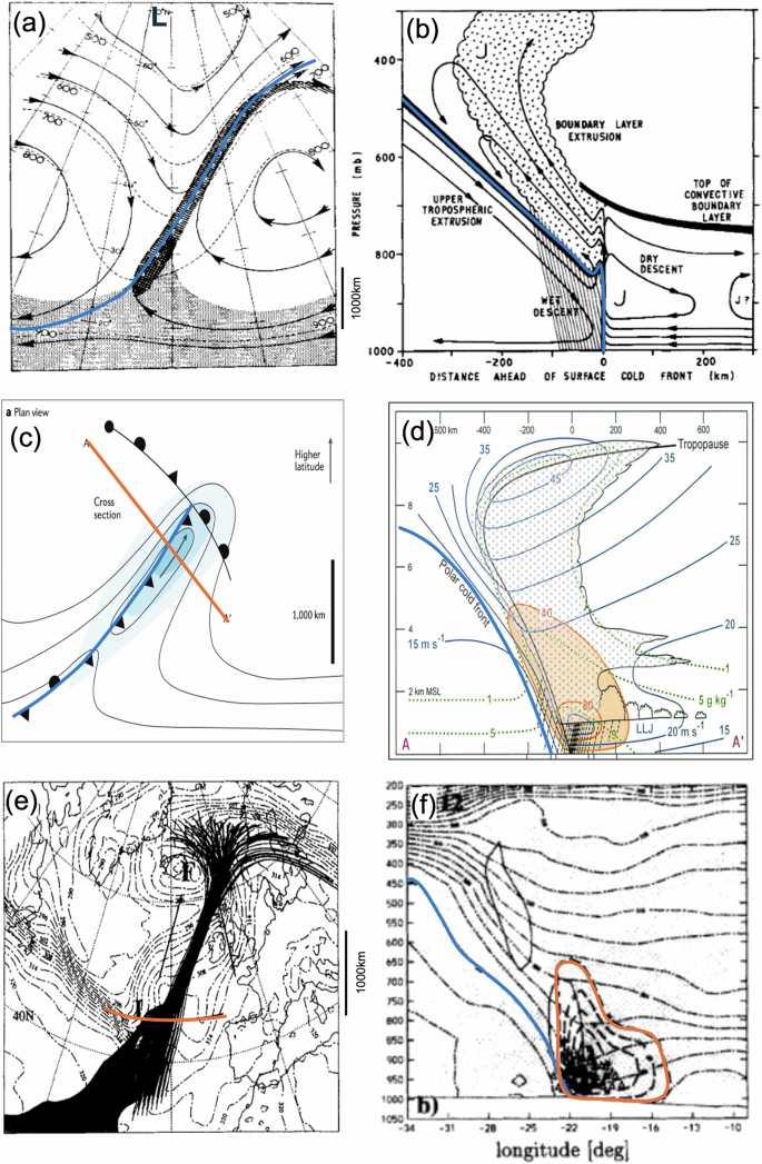
a Plan view of isentropic ETC-relative streamlines (arrows), isentropic surface height (dashed), cold front (overlaid blue), moist air (light grey) and clouds (dark grey) from33. b Vertical cross-section of ETC-relative streamlines (arrows) across an ana-cold front, cold front (overlaid blue), saturated ascent (stippled), upper and low-level jets (labelled J) from36. c Plan view of an AR identified as region of high IVT (blue shading), TCWV (black contours), cold front (overlaid blue) from82. d Vertical cross-section through AR, water vapour flux (orange shading), specific humidity (green dashed), windspeed (blue) showing position of LLJ, cold front (overlaid blue thick) and cloud (stippled). e Coherent ensemble trajectories with high water vapour flux, mslp (dash-dot), position and motion (arrow) of low pressure centre 48 hours apart from38 f Vertical cross-section through trajectories with potential temperature (dash-dot), cold front (blue overlaid), high water vapour flux (dashed) from38.
From a Lagrangian perspective,38 identify coherent ensembles of trajectories using ascent larger than 620hPa, decrease in specific humidity greater than 12 g kg−1 and time-mean water vapour flux greater than 0.17 m s−1. The 3 criteria thus identify subtly different sub-regions of the WCB flow. One cluster ascends up the warm frontal surface and turns anticyclonically to form a cirrus shield (known as W1 or the forward-sloping WCB39) another ascends rapidly on the warm side of the cyclonically turning bent-back front forming the cloud head of an ETC (known as W2 or the rearward-sloping WCB39) and a third originates in the warm sector boundary layer, remains ahead of the cold front and ascends reaching the middle troposphere only in the later phase of its development. This third coherent WCB ensemble corresponds to an AR (i.e. within a region of large vertically integrated water vapour flux). Both W1 and W2 clusters remain close to the ETC centre during its development, so are roughly stationary in an ETC-relative framework until they ascend into the cloud head. The AR trajectories are only located in the region of high water vapour flux for a short period, demonstrating that an Eulerian AR feature marks a region of rapid passage rather than constituting a Lagrangian entity. Figure 6e and f show equivalent plan view and vertical cross sections to Figure 6a–d but for coherent ensembles of Lagrangian trajectories from38. These trajectories satisfy the criteria of 48 hour average water vapour flux greater than 0.17 ms−1 designed to identify the AR part of the WCB. The coherent ensemble of trajectories is narrow (200 km) close to the UK before fanning out north of 60∘. The trajectories start in the ETC warm sector with ascent in the later stages and reaching only to the mid-troposphere in the warm front region. Figures 6f shows a west-east orientated vertical cross-section through the coherent trajectories. It is shown that these trajectories are located just ahead of the cold front in the region of a low-level jet (winds up to 40 ms−1). Thus in this fully Lagrangian framework, it is clear that the AR and WCB structures are the same.
In summary, both Eulerian and Lagrangian methods can be used to identify WCBs and ARs. Broadly speaking their structure and evolution are all consistent, suggesting that they are both different perspectives of the same synoptic feature.
Dynamical description of of ETC and AR development
Many significant features of the atmosphere cannot be fully explained by quasi-geostrophic theory. Among them are strong ETC fronts and low-level jets, across which the horizontal scale is usually 100km or less. A front is a boundary between two airmasses, frequently defined in terms of temperature, but also density, moisture, potential temperature and equivalent potential temperature. A low-level jet is an intense narrow, quasi-horizontal current of wind associated with strong vertical shear. Fronts and jets are dynamically related since differences in the thermal (or more strictly, buoyant) properties of airmasses on either side of a front leads to vertical shear of the geostrophic wind along the front. Thus, a front implies a jet (or, at least, a jet in the feature-relative flow).
Fronts do form in quasi-geostrophic theory; but the geostrophic strain flow causes a pre-existing horizontal temperature gradient to increase by an order of magnitude over a period of around 2.5 days (40, p298,41, p361). Thus the kinematic action of geostrophic strain on a temperature gradient is an incomplete explanation of observed frontogenesis, which occurs much more rapidly. Quasi-geostrophic theory therefore shows that strain can strengthen temperature and moisture gradients, but a less-approximate version of the governing fluid-dynamical equations, known as semi-geostrophic theory, is needed to account for their rapid intensification on synoptic timescales7. In semi-geostrophic theory it is assumed that the winds in the along-front direction are approximately geostrophic, but in the cross-front direction they are not. The non-geostrophic component of the flow is known as the ageostrophic wind. If we divide the total wind field into a part that contains divergence and a part that does not, the non-divergent part is approximately geostrophic, thus the ageostrophic wind is largely responsible for convergence and divergence in the atmosphere. Strictly speaking, the geostrophic wind is non-divergent but not the other way around.
If a horizontal temperature gradient increases through geostrophic strain, the difference between the geostrophic wind at upper altitudes minus that at lower altitudes (known as the thermal wind) must increase to maintain thermal wind balance. To increase the thermal wind, the geostrophic wind accelerates in the upper atmosphere and decelerates near the surface. Since the ageostrophic component of the wind is perpendicular to the parcel acceleration, the ageostrophic wind aloft is from the warm to cold side of the front and below from the cold to warm side of the front with the largest magnitude co-located with the strongest temperature gradient. Due to continuity considerations, there is convergence and rising motion near the surface on the warm side of the front (strengthening the ascending part of the WCB42) and convergence and sinking motion aloft on the cold side of the front (known as the dry intrusion). Rising motion in the ETC warm sector and sinking motion in the ETC cold sector results in a conversion of potential energy into kinetic energy and an increase in the windspeed (strengthening the flux of moisture in the AR). The cross-front ageostrophic advection of temperature causes frontogenesis on the warm side of the initial gradient near the surface and the opposite aloft resulting in a tilt in the isentropes. Hence, the ageostrophic circulation tilts the frontal zone and increases the rate of frontogenesis at the surface and the near surface discontinuities at the front illustrated in fig. 6. This increased frontogenesis rate acts to sharpen the moisture gradients at the edge of ARs, and the enhanced ascent in the WCB explains observed precipitation rates. Thus, it is necessary to include ageostrophic motions in any dynamical theory explaining the development of ARs.
AR studies such as16 also describe the convergence of low-level winds towards the cold front. A relationship between ARs and the most rapidly deepening ETCs is suggested by43, and, the convergence of low-level winds is examined. They show patterns of low-level convergence along lines on scales of many thousands of km and “the low level divergence patterns provide one approach to the classification of boundary layer air into ‘air masses’. More recently,44 investigated the evolution of two zonally elongated ARs in an environment characterized by strong frontogenesis and20 studied a climatology of ARs and produced composite ARs that highlighted the relationship between frontogenesis processes and meso-scale secondary ageostrophic circulation across ARs. Thus, many AR studies have confirmed that ageostrophic motions are necessary for the formation and elongation of ARs.
Kinematic description of ETC and AR development
In this section, we use kinematic analysis and schematic diagrams to illustrate the effect of ageostrophic motion (convergence) on the further evolution of the AR. Figure 4b shows composite ETC-centred fields in the developing stages of ETC development (24 hours before maximum ETC intensity). By this time the frontogenetic strain (described in the previous section on Kinematic description of cyclogenesis and tropical moisture exports) has tightened the frontal temperature and moisture gradients along the cold front. Figure 5b shows that the background flow continues to advect fluid parcels ahead of the cold front towards the north-east. The ETC mean flow also continues to advect the air parcels cyclonically around the low centre. The rotational and convergent components of the flow along the cold front have increased while the frontal strain component along the cold front remains positive far from the ETC centre but is negative close to the ETC centre. As described in the sections on Dynamical description of of ETC and AR development and Synoptic description of ETC and AR development, rapid frontogenesis is the result of (ageostrophic) convergent wind ahead of the cold front leading to a tight temperature gradient far from the ETC centre 24 hours later (Fig. 4c), and strengthened ascending motion in the WCB. Close to the ETC centre divergence and negative frontal strain leads to a weakening of the moisture and temperature gradients (frontolysis). The cold front becomes disconnected from the warm front (frontal fracture) and moves perpendicular to the warm front as the ETC develops. Thus, in addition to translation by the ETC, background flow and strain components of the flow described in figure 3(c), we add convergent flow ahead of the cold front. To compensate for horizontal convergence at low-levels there is divergence of the air parcel in the vertical. Ascending moist parcels reach saturation as they expand and cool leading to the formation of clouds and precipitation removing moisture from the atmosphere. This kinematic analysis 24 hours before maximum ETC intensity is used as the basis for the evolution of the TCWV field in Fig. 3d which illustrates the extension of the filament of TCWV into the midlatitudes, a decrease in its magnitude due to precipitation (orange shading) and the development of a T-bone frontal structure as described by45.
At the time of maximum intensity, Fig. 5c, convergent flow acting on a moist parcel close to the ETC centre causes the fluid parcel to contract and rotational flow causes the moisture filament to wrap further around the low centre. Finally, the frontal strain acting on the moist air parcel causes it to become elongated in the along front direction. Precipitation quickly depletes the moisture content of the column. However, in a moist environment, there is continuous convergence near the ETC centre which partly replenishes the moisture lost via precipitation, while also enhancing the ascent leading to further precipitation. This kinematic analysis at maximum ETC intensity is used as the basis for the evolution of the TCWV field in Fig. 3e and f which illustrates the anticlockwise spiralling of the TCWV filament around the ETC centre, which is often observed when the ETC and the tip of the AR reach the midlatitudes.
As a result of continuous convergence at low-levels (Fig. 5c), even if the ETC propagates with a velocity that is faster than the low-level background wind speed, the filament of moisture can continue to extend into the extratropics due to continuous moisture flux convergence ahead of the ETC cold front (Fig. 3e). In the later stages of ETC development the filament of moist air begins to spiral around the low centre due to the continued action of cyclonic motion on the air parcels (Fig. 5c, d). The trajectory taken by these moist air parcels is consistent with the W1 cyclonically turning WCB airflow described by38. Note that in the decaying stage of ETC lifecycle (Fig. 4d) the cold front and AR is often located >1000 km from the ETC centre. While the strain becomes negative close to the ETC centre it remains positive along the trailing cold front thus continuing to create strong moisture/temperature gradients far from the ETC centre and thus a coherent AR structure in the subtropics even when the ETC centre has moved into the midlatitudes. Subsequent ETCs (secondary cyclones) can form on this trailing cold front.
Diabatic heating, secondary cyclogenesis and ETC/AR families
In this section, we consider the mature and decaying stages of ETC lifecycle during which fronts can become unstable leading to secondary cyclogenesis. We start with a synoptic description of these features, followed by a dynamical description and end with a kinematic synthesis providing a bridge between the synoptic and dynamic descriptions. We use the kinematic synthesis to further extend the schematic diagram illustrating the lifecycle of an AR to include AR families.
Synoptic description of diabatic heating, ETC and AR families
Multiple ETCs developing on the same frontal zone form what is known as a family of ETCs4. Figure 7a and b shows one such family of 5 ETCs in the North Atlantic. Each ETC is identified with a mean sea level pressure minimum and a cyclonic comma-shaped cloud feature. The first ETC in an ETC family is known as a primary or parent ETC, with subsequent ETCs referred to as secondary ETCs. Each of the ETCs in an ETC family typically follows a similar track, steered by the planetary-scale wave flow. In recognition of the fact that not all ETCs in rapid succession form on the same frontal zone, the term ETC clustering has been introduced more generally, as a period of time during which a certain location is affected by an anomalously high number of ETCs. Thus ETC families and ETC clustering periods can cause significant impacts due to successive days with high precipitation or strong winds46.
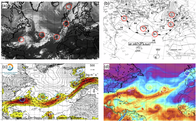
a Infrared satellite image, b NCEP surface analysis chart showing mslp (contours), surface fronts and position of surface high (H) and low (L) pressure centres, c Centre for Western Weather and Water Extremes showing the magnitude of IVT (coloured shading), the direction of IVT (arrows) and mslp (black contours). d Microwave satellite total column water vapour (TCWV). Figures overlaid with the position of the family of ETCs (circles). Colourbars have been deliberately removed to focus on position of ETC family and frontal features with respect to AR family without dependence on criteria for identifying them.
The phenomena of AR families was introduced by47, defined as two or more AR events occurring within one aggregation period. The AR’s in an AR family may or may not be part of the same filament of high moisture transport. Thus, this definition is analogous to the broader concept of ETC clustering than ETC families. Figure 7c and d shows the equivalent IVT and TCWV fields for the same time as Figures 7a and b. The ETCs are all located on the northern edge of a filament of high TCWV, which extends the entire way across the north Atlantic (fig. 7d). Multiple maxima in IVT occur along this AR filament (Fig. 7c), which may constitute a family of ARs or multiple ETCs forming on a single AR (such as described by44), depending on the criteria used to identify ARs.
The role of moisture in ETC development has been studied in the ETC literature. In ETCs, latent heat release occurs when moist air ascends and water vapour condenses and, at higher altitudes, freezes causing latent heat release48. Latent heat release is a particularly important factor in the intensification of secondary ETCs.49 showed for a case study ETC that strong diabatic heating can increase the slope of isentropic surfaces in the mid-troposphere and thus increase environmental baroclinicity favouring the development of subsequent ETCs. Several AR studies have confirmed the importance of latent heating in ETC development via the statistical relationship with AR strength. For example,50 observed that intense ETCs are often preceded by the presence of ARs, indicating their role in promoting explosive ETC development. Similarly51 found that nearly 80% of explosive deepening ETCs are associated with ARs, suggesting a significant connection between ARs and explosive cyclogenesis.52 also showed that greater ETC intensification occurs with stronger ARs, suggesting that ARs enhance ETC deepening by providing more water vapour for latent heat release. However, in order for moisture to contribute to cyclogenesis, a mechanism for creating ascent is necessary. Without ascent, moisture remains passive and unable to release its potential energy to fuel the cyclogenesis process.
ETC clustering periods have also been associated with the presence of an extended and intensified upper-level jet, maintained by upper-level synoptic-scale wave breaking53,54,55. Wave breaking at upper-levels (often termed Rossby wave breaking) occurs when a wave in the upper-troposphere amplifies beyond its linear growth phase and overturns. The direction of wave breaking is influenced by the upper-level wind shear. Thus anticyclonic wave breaking typically occurs on the equatorward side of the jet and cyclonic wave breaking occurs on the poleward side of the mean jet. Wave breaking causes energy to be transferred from the ETC to the mean flow, acting to accelerate the jet. This enhanced jet steers subsequent ETCs more rapidly over the same location (leading to ETC clustering) and reduces the atmospheric stability providing a favourable environment for the intensification of secondary ETCs. Recent studies have also investigated the connection between upper-level wave breaking and the frequency and persistence of ARs.56 discovered that prolonged AR events along North America’s western coast, lasting over 63 hours, are linked to anticyclonic wave breaking at upper-levels. Similarly57 found that 73% of the AR events they studied are related to anticyclonic wave breaking.
Dynamical description of diabatic heating, secondary cyclogenesis and ETC/AR families
In dynamical analysis, the role of diabatic heating can be incorporated into the simplified equations (quasi-geostrophic/semi-geostrophic) used to describe atmospheric motions in a moist atmosphere. In ETCs, diabatic heating occurs when moist air ascends and water vapour condenses causing latent heat release48. This latent heat release can impact the dynamical wind field in the atmosphere. Potential Vorticity (PV) is a useful means for identifying the dynamical feedbacks associated with latent heat release in the free troposphere. PV combines the absolute vorticity and stratification in the atmosphere.
The moist quasi-geostrophic PV equation58 describes how the PV in the atmosphere evolves due to advection by the geostrophic wind and is modified by diabatic heating/cooling. Thus, in the absence of diabatic heating, quasi-geostrophic PV is conserved along geostrophic flow trajectories. Diabatic heating or cooling changes the static stability and modifies the PV distribution leading to changes in the atmospheric flow. Moist quasi-geostrophic models show that as the diabatic heating rate increases, the ETC wave growth rate increases, ETC wavelength decreases and ETC propagation speed increases59,60. Furthermore, in moist semi-geostrophic models, latent heat release leads to an increase in the rate of surface frontogenesis (and hence narrower and more intense ARs) and reduces stability leading to faster ascent in the WCB61 (see ref. 62 for an excellent review of the role of diabatic processes on ETC development.)
Condensation of moisture in frontal convection or ascending part of WCB airflows generates heating, reducing stability and creating a region of anomalous positive PV below the heating maximum. Under the influence of the Coriolis force, this results in a cyclonic circulation which can enhance the existing cyclonic vorticity in an ETC causing it to become more intense (known as diabatic forcing). The strengthened ETC can then further increase ascent, moisture transport and subsequent latent heat release, creating a positive feedback loop that intensifies the ETC, WCB and AR. The extent to which diabatic forcing contributes to the overall intensification of a WCB and AR varies, with some ETCs strongly dependent on the presence of moisture. ETCs strongly influenced by diabatic heating are known as type C ETCs63,64,65 (or diabatic Rossby waves) and they often form in regions of low static stability. Their intensification is sensitive to the magnitude of low-level PV during their development phase66,67.
In61, their moist semi-geostrophic model found that latent heat release produced a line of PV along the frontal surfaces of an ETC. Mesoscale-waves forming along the edges of such horizontally orientated PV strips can interact initiating cyclogenesis11,68,69 via a mechanism known as barotropic instability. Barotropic instability extracts kinetic energy from the horizontal wind shear in the mean flow allowing the edge waves to grow. If these mesoscale waves amplify, the PV strip can break up into individual anomalies and the cyclonic circulation associated with these anomalies can lead to the formation of shallow ETCs forming along the cold front or occasionally the occluded front of the preceding ETC (known as frontal waves)65,70,71,72. If these low-level PV anomalies couple with upper-level synoptic-scale waves both the upper-level wave and the low-level frontal wave can amplify further leading to a deepening of the frontal wave into a synoptic-scale ETC with their own ETC fronts, WCBs and ARs (known as secondary cyclogenesis).
The break up of diabatically generated PV into individual anomalies is influenced by frontogenetic forcing, arising from strain flow at the frontal boundaries. In their semi-geostrophic model,73 found that strain (Fig. 1) can compress secondary frontal waves across the front and stretch them along the front. Large strain rates impede secondary ETC amplification, with frontal waves failing to amplify when strain rates surpass 0.6 × 10⁻⁵s−1 12. These findings were confirmed in idealised modelling studies using the primitive equations (no assumption of geostrophic balance in the horizontal momentum equations)65 and a climatological study of secondary frontal wave cyclogenesis by67. Similarly, in a climatology of 192 ARs74 found that highly frontogentic cases produce local maximum in lower-tropospheric PV that may intensity the prefrontal low-level jet and enhance water vapour transport and IVT within the AR. Thus, ascent of moist air can generate a positive PV strip along an ETC cold front, which may become unstable if the strain acting on the front decreases.
Kinematic description of ETC and AR families
In this section, we use schematic diagrams to illustrate the development of ETC and AR families. Figure 3f shows the development of a frontal wave (secondary ETC) on the trailing front of the decaying primary (or parent) ETC. Secondary ETCs often form beneath the right entrance of an upper-level synoptic-scale jet streak where upper-level divergence enhances ascent rates in the mid-troposphere. An air parcel ahead of the trailing cold front will be subject to translation by the background flow and a strain flow which enhances the low-level temperature gradient (Fig. 4b). This strain flow can also change the shape of the air parcel, stretching it along the axis of dilatation and compressing it along the axis of contraction. If the strain acting on the front remains strong, it may suppress the growth of the surface frontal wave, but if it weakens the frontal wave can amplify and couple with the upper-level shortwave into a synoptic-scale ETC. Convergence along the primary ETC cold front can increase the moisture gradient ahead of the secondary ETC and a ‘secondary’ AR can form linked to this enhancement of the TCWV or IVT.
Since the preceding ETC has created a region of enhanced moisture, the secondary ETC is forming in a moisture-rich environment.75 investigated cyclogenesis differences in ETCs with and without nearby ARs, revealing that ETCs beginning with preexisting ARs receive significantly more water vapour inflow, intensifying ETC deepening. Thus it is hypothesised that the enhanced moisture ascending in the secondary ETC WCB may boost the dynamical intensity of the secondary ETC, further enhancing the secondary AR. However, to the authors knowledge this hypothesis has yet to be fully tested.
Secondary ETCs can develop explosively as they cross the upper-level jet axis and enter the left exit region. The trailing cold fronts associated with the secondary ETC can itself become unstable and further ETC develop creating the family of ETCs and ARs.
Discussion
The research methods used to investigate ETCs, WCBs and ARs are varied but they can broadly be categorised into studies utilising synoptic analysis, which have a focus on the physical attributes of these features, and dynamical analysis, which focuses on the mechanisms responsible for their evolution. This paper adopts a kinematic perspective to reinterpret mid-latitude synoptic and dynamical research, aiming to integrate various concepts. Our analysis shows that, although there are discrepancies in methods, definitions, and terminology used to describe extratropical cyclones, warm conveyor belt airflows, and atmospheric rivers, the fundamental mechanisms behind their formation and evolution remain consistent. While it is useful to study these phenomena independently, it is crucial to understand that they are interconnected within a larger atmospheric flow pattern. Through kinematic analysis, we develop schematic diagrams that illustrate the lifecycle of an AR. Differences in the language and tools used has inevitably led to difficulties comparing and contrasting results from different studies and to several common myths in the literature which are addressed here.
-
Myth 1: WCBs and ARs are distinctly different synoptic features
-
WCBs and ARs in the extratropics are components of larger-scale propagating wave patterns. They are the result of the same strain and convergent flow fields that generate strong fronts and pre-frontal low-level jets (LLJs). AR studies have traditionally focused on their role in transporting moisture poleward, which is why AR identification typically relies on 2D Eulerian criteria. In contrast, WCB studies examine both the horizontal and vertical transport of moisture that leads to cloud formation and precipitation near propagating ETCs, hence the use of 3D quasi- or fully Lagrangian criteria to identify WCBs. Misunderstandings often arise concerning the extent of these features along the cold front. AR definitions typically emphasise their long and narrow shape, while some WCB studies focus on the ascending part of the flow near the ETC center. However, while the longer TCWV filament is often visible extending into the subtropics, there is a clear downstream strengthening of TCWV flux (IVT) near the ETC center, which coincides with the pre-frontal WCB airflow. Overall, ARs and WCBs appear to be part of the same structure, generated by the same mechanisms, and can be considered interchangeable terms, disregarding their specific identification criteria.
-
-
Myth 2: Midlatitude precipitation is caused by moisture transported directly from the tropics
-
The moisture flux within ARs typically runs parallel to the cold front of an ETC and is often directed from the subtropics toward regions experiencing heavy precipitation in the extratropics. This often leads to the assumption that moisture is transported over long distances directly from tropical source regions, giving rise to the term “tropical moisture tap” to describe ARs. However, this notion obscures the fact that ARs are part of dynamic wave patterns that move relative to the flow in which they are embedded. Thus, for AR features travelling at, or faster than, the mean low-level flow, moisture at the subtropical origin of an AR cannot contribute to precipitation at its midlatitude endpoint even after some elapsed time. This is because the endpoint of the AR advances more rapidly than the individual air parcels within the AR. To sustain the high TCWV levels at the AR’s leading edge as it moves poleward, continuous local moisture flux convergence along the AR’s path is required. While some of the moisture precipitating in the extratropics may have evaporated in the subtropics, the majority originates from the local environment, where strain and convergent flow fields near the center of the ETC lead to the extension of moisture filaments.
-
-
Myth 3: ARs cause cyclogenesis
-
The ascent of air, which is essential for ETC development, is primarily driven by large-scale upward motion within the planetary-scale trough and ridge system. ETC development is further enhanced by smaller-scale frontogenetic processes, such as strain and convergence, which intensify horizontal temperature gradients and lead to front formation. Low-level convergence forces air masses to rise, creating conditions where moisture can contribute to ETC strengthening through condensation and latent heat release. However, latent heat release is generally not the primary cause of cyclogenesis (with the exception of relatively rare diabatic Rossby waves). Without the large-scale and frontogenetic mechanisms that trigger ascent, moisture remains passive and unable to release its potential energy to fuel the cyclogenesis process. Therefore, while moisture plays a role in enhancing and sustaining cyclogenesis, the initial upward motion is driven by dynamic atmospheric factors. Additionally, it is the presence of moisture, rather than its flux along the AR, that is important in strengthening ETCs. This is consistent with the observation that secondary cyclogenesis is often associated with a weakening of along-front strain flow and, consequently, a weakening of AR flow.
-
Methodology
In this study, we use the ERA-Interim reanalysis dataset. ERA-Interim provides a detailed representation of the Earth’s atmosphere by assimilating observational data from various sources, including satellites, weather balloons, and ground stations76. The atmospheric parameters used in this study include total column water vapour and 850 hPa potential temperature (θ), relative vorticity and horizontal wind fields, extracted on a latitude-longitude grid with a resolution of 0. 7∘ × 0. 7∘. Higher-resolution datasets are available, but for our study, calculating the derivatives needed for the kinematic flow decomposition from higher resolution data results in noisy fields, so some smoothing is required to reveal the synoptic structures we are interested in, therefore ERA-Interim is preferred for this study.
Following the method of77, we use a quasi-Lagrangian method and track the 200 most intense north Atlantic ETCs over a 20-year period (1989-2009) using an ETC tracking algorithm78. The tracking was conducted during the winter months (December-January-February) using 3-hourly 850 hPa relative vorticity data. As relative vorticity can be noisy, we applied a spectral truncation to T63, corresponding to a Gaussian grid resolution of approximately 1.88∘ at the equator, before tracking. To ensure we focused on ETCs, short-lived (<48 hr) or stationary features (<1000 km travel) were excluded. Cyclogenesis is defined as the first point in each ETC track, and ETC intensity is measured using maximum T63 vorticity.
For the compositing process, we obtained ERA-Interim data at 24-hour intervals, relative to the ETCs time of maximum intensity, capturing atmospheric conditions within a 20∘ radius of each ETC centre. Following79, ETC composites were created by averaging fields after rotating them to align with the ETC’s direction of travel. This rotation is essential, as it aligns mesoscale features like warm and cold fronts that could otherwise be smoothed out during compositing. For plotting, the composite fields are rotated by the average propagation direction so that north is at the top of the figures. Only the 200 most intense ETCs were included in the composite to ensure homogeneity in their development, though this focus may bias the results toward representing the most extreme ETCs.
To explore the role of the flow field in controlling the strength and shape of ETC fronts and ARs, we calculated the contributions of each component of the flow for every grid box within 20∘ of the ETC centre. The mean flow can be split into a part related to planetary-scale variability and a part related to synoptic-scale variability using temporal spectral analysis. The low-frequency part of the 850 hPa wind field that varies with time periods greater than 8 days is denoted the Background translational flow, ub. The high-frequency part of the 850 hPa wind field that varies with time periods less than 8 days is denoted the ETC translational flow, uc. It has horizontal components uc and vc in the zonal (x) and meridional (y) directions.
The derivative components of the flow are given by;
Δλ is the horizontal length scale over which rotation, convergence and strain are acting (see Fig. 1). This is approximately twice the horizontal grid-spacing in the mid-latitude ERA-Interim dataset (Δλ =150 km). To determine the action of strain on local temperature gradients, the strain along the axis of dilatation and contraction is projected onto the local along and across-isotherm directions respectively to give the frontal strain flow (Fig. 8). Derivations of this can be found in many dynamical meterology textbooks including9 (their equation 7.11) and40 (their equation 2.3.19).
Note that the total horizontal rate of frontogenesis, as analysed by80,81 is a combination of convergence across the front and the frontal strain flow.
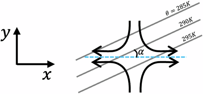
The angle α is the angle between the axis of dilatation (dashed cyan) and the isotherms (grey).

Responses