Carbon uptake of an urban green space inferred from carbonyl sulfide fluxes

Introduction
As a consequence of climate change, cities seek ways to carbon neutrality. In order to verify carbon emission reductions, atmospheric measurements are crucial. Measurements of greenhouse gas concentrations and emissions can be made with many different methodologies and in a variety of scales extending from local-scale eddy covariance (EC) measurements1,2 to city-level tall tower and total column measurements3,4,5. From the different observational methods, EC is the most direct technique to quantify urban emissions by providing the carbon dioxide (CO2) net exchange (NEE) between a land area and the atmosphere almost continuously. However, partitioning NEE into different flux components is critical to quantifying the anthropogenic emissions and for a comprehensive understanding of the contribution of urban areas to climate change. One of these components is the carbon assimilation, i.e., gross primary production (GPP) of urban vegetation, which takes up part of anthropogenic emissions and thus obscures emission signals6. In the absence of anthropogenic emissions GPP can be estimated by subtracting ecosystem scale respiration (R) and NEE (see GPPEC in Eq. (7)). In a human-influenced context, however, CO2 emissions cannot be neglected, but they reveal a pitfall of the simple GPPEC methodology: It cannot recognize which NEE data have been influenced by anthropogenic CO2 emissions, and thus cannot be used in an urban context. Consequently, measurements of urban GPP have been residual estimations7 or are based on light-response curves8, but direct observations have been missing.
Carbonyl sulfide (COS) is a gaseous compound naturally found in the atmosphere, with an average mixing ratio between 440 and 500 ppt9 (10−12 mol COS per mol dry air). COS is taken up by the plants through their stomata, and its exchange is closely related to the stomatal conductance of vegetation10. However, as COS shares the same entrance pathway to the leaf with CO2, a connection between biogenic COS uptake and GPP can be created11. COS is destroyed at the chloroplast surface by the enzyme carbonic anhydrase (CA) in a hydrolysis reaction, and unlike CO2, is not respired back to the atmosphere as a part of plant metabolism10. GPP has been estimated from COS fluxes on vegetated environments12,13,14, but its potential has not been harnessed in human-influenced environments. Urban EC fluxes of COS have been studied before over a few weeks in Innsbruck15, where the main conclusion was that better information on anthropogenic sources is still needed to properly utilize COS as a proxy for GPP in this highly built source area. The same conclusion was obtained by two recent flask sampling studies conducted in Barcelona, Spain16 and Lutjewad, the Netherlands17. They observed notable influence from maritime and industrial sources of COS preventing making solid estimation of GPP.
In this study, we report the first EC fluxes of COS measured over a full growing season in Helsinki, Finland, in an urban area that also has a significant vegetated cover fraction (Figs. 1c, S1, and Table S1). This allows us to examine both biogenic and human-influenced trace gas fluxes in a setting that narrows the gap between the fully vegetated and the heavily built areas studied before. We study the impact of anthropogenic activities in the study area by comparing COS and CO2 fluxes with carbon monoxide (CO) fluxes, which have been used as an indicator of anthropogenic emissions of CO2 from combustion processes1. We show how COS fluxes can be used to derive urban GPP using two different approaches and use it to calculate anthropogenic CO2 emissions from NEE.

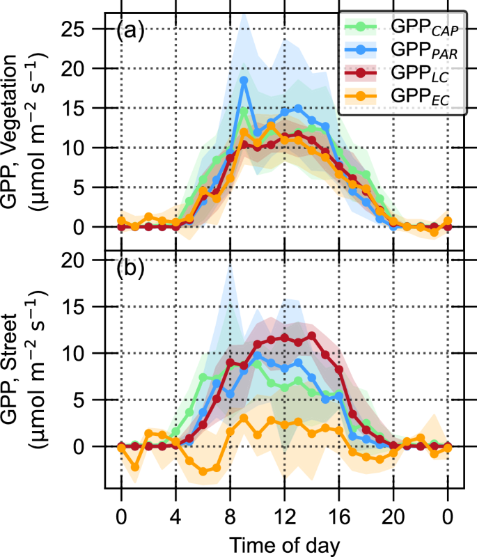
The top panels show the number (N) of available quality-checked flux data for each gas every hour of the day. Dotted lines in a and (b) show the median diurnal fluxes and the shadowed areas indicate interquartile ranges of the fluxes. Each flux magnitude is shown on the same y-axis, but the units are different, as indicated in the legend. Panel (c) shows the land use around the EC tower, see more details in Fig. S1.
Results and discussion
Trace gas fluxes during growing period
CO, COS, and CO2 fluxes in street and vegetation sectors display notable deviations as a consequence of different surface cover fractions and human activities (Figs. 1 and S2). Both sectors function as sinks of COS reaching the highest hourly median uptakes of −10.6 and −19.7 pmol m−2 s−1, respectively. To compare, the mean daytime uptake of −23.5 pmol m−2 s−1 was observed in a deciduous forest during June, August, and September18, whereas the daily maximum uptake varied between −24 and −33 pmol m−2 s−1 during different years in a boreal coniferous forest19. When the sectors are examined together, a clear positive correlation between COS and CO2 fluxes is observed, with an uptake ratio of 0.86 pmol μmol−1 (R2 = 0.39; Fig. S3a). When only times with simultaneous COS and CO2 uptake are considered and placed on a similar scatter, the uptake ratio becomes 1.67 pmol μmol−1 (R2 = 0.52; not shown). This closely agrees with earlier reported values from leaf chamber measurements in a controlled greenhouse environment, where the ratio was 1.41 pmol μmol−1 11. This shows the applicability for estimating GPP from COS fluxes at our site, since the methodology relies on the simultaneous uptake of both gases (Eq. (3)).
The street sector is a source of CO2 with diurnal median values varying between 2.3 and 6.5 μmol m−2 s−1. The vegetation sector is on median a CO2 sink between 8 a.m. and 5 p.m. reaching −6.6 μmol m−2 s−1, consistent with previously reported estimates (ca. −7.7 μmol m−2 s−1)20. Nocturnal CO2 sources are larger on the vegetation than the street sector likely due to soil and vegetation respiration. However, the daytime uptake in the vegetation sector offsets the nocturnal emissions, which is not the case in the street sector. When summed over a median day of the growing period, the vegetation sector sequestrates −8.0 gCO2 m−2 d−1, comparable with −4.6 gCO2 m−2 d−1 observed in Baltimore8, whereas the street sector emits 392.4 gCO2 m−2 d−1. CO2 and CO fluxes are also significantly correlated during daytime (R2 = 0.74, p < 0.001, Fig. S3b) but not nocturnally. Strong correlation originates mainly from road transportation on the street sector, since there are no other combustion processes taking place in similar scales.
The street sector CO and CO2 fluxes behave differently than corresponding fluxes in the vegetation sector because of transportation in the source area. The daily median CO source of 23.1 nmol m−2 s−1 originating from, on average 25,000 daily passing cars is comparable to the lowest observed CO fluxes in central London (16.9 nmol m−2 s−1)21. In the vegetation sector, the median daily emission is 7.5 nmol m−2 s−1, which still is higher than would be expected in a fully vegetated environment. A boreal forest emitted up to 1.6 nmol m−2 s−1 22, and the highest monthly mean on a grazed grassland was 1.9 nmol m−2 s−1 23. Construction work on a tram line has taken place in the vegetation sector, which can explain large parts of the CO emissions. In addition, there may be some other unknown fossil fuel emissions in the vegetation sector such as local wood burning in the allotment garden or site machinery in the botanical garden. Also, another important access road 800–900 m from the tower, can influence the CO fluxes coming from the direction of the sector particularly at night-time when the atmosphere is stable and the source area extends longer. The impact is, however, not visible on CO2 and COS fluxes due to the large mass of vegetation separating the road from the EC tower.
The EC measurement of COS flux in Innsbruck showed a day-time source, which was connected to exhaust fumes and tire wear of vehicular transportation15. A similar deduction was made in Beijing, where tire wear was conjectured the single largest source of COS during summertime24. If an anthropogenic COS source originated from vehicular fuel combustion, a clearer relationship between COS and CO fluxes would have been seen, as is the case with CO2. There is no statistically significant dependence between COS and CO fluxes (Fig. S3c) indicating mostly negligible anthropogenic COS emissions. Thus, our results do not support the earlier findings about COS emissions originating from tire wear. However, slight anthropogenic influence cannot be disregarded, particularly in the road sector causing some level of uncertainty in our analyses.
Novel estimation of urban GPP
During the brightest hours (photosynthetically active radiation PAR >700 μmol m−2 s−1), the leaf relative uptake (LRU, see the “Methods” section) needed to estimate GPP from COS flux had medians of 1.12 (interquartile range 1.0–1.3) and 1.45 (1.3–1.5) in the vegetation sector, as determined with PAR and CAP methods, respectively. These values compare well with 1.68 obtained for natural ecosystems in a review study25. LRUPAR smoothly decreases with PAR, whereas LRUCAP saturates earlier by PAR and has a wider range of values on a single PAR due to the moisture conditions—namely vapor pressure deficit (VPD) and soil water content (SWC)—being taken into account (Fig. S4a).
The four methods used to estimate GPP (GPPCAP and GPPPAR based on COS measurements, GPPLC based on a light-response curve, and GPPEC based on carbon balance partitioning by respiration) provide a similar, qualitatively expected performance on the vegetation sector with the largest uptake in daytime and (near) zero at night-time (Fig. 2a). GPPPAR yields the highest median biogenic uptake of 18.5 μmol m−2 s−1 whereas with other methods the peak median values remain between 11.7 and 14.6 μmol m−2 s−1. GPPEC results in some slightly negative nocturnal GPP values as a consequence of uncertainty in ecosystem respiration (R) by the simple model used in this study. The estimated mean R (3.9 μmol m−2 s−1) agrees with the measurements conducted in Boston metropolitan area26 [2.6–6.7 μmol m−2 s−1], but yield lower values compared to chamber measurements conducted in the vegetation sector in an earlier study27 [5.5–6.1 μmol m−2 s−1]. In the latter, the chamber measurements were only made from lawns and meadows and thus did not present all soil and ground vegetation types within the vegetation sector.
Panel (a) shows the diurnal cycle on the vegetation sector and panel (b) shows it on the street sector. Data were collected between May 1 and October 10, 2023. Only moments with data available from all methods were used. Dotted lines show the median diurnal cycle and the shadowed areas in the interquartile range. Note different scales on y-axes.
The COS-based GPP estimations match well with GPPEC and GPPLC which are the more traditional methods to estimate GPP from EC measurements in vegetated ecosystems. GPPLC is essentially a parameterization of GPPEC as a function of PAR. Thus, the light response curve estimation of GPP can be used as a reference value for photosynthesis where there is a distinct and well-defined green sector. Also, GPPLC works well against the small and occasional anthropogenic contributions visible in GPPEC due to the averaging nature of parameterization. However, without the near-pure biogenic signal, GPPLC cannot be parameterized, which becomes an essence of the NEE partitioning problem in urban areas.
GPPCAP and GPPPAR provide an independent mean to estimate GPP, but as both rely on COS concentration and flux measurements, they show more variability with similar peaks than the other two methods. GPPPAR reaches higher peak values and shows steeper changes in both morning and evening hours, as PAR is considered the only limiting factor of LRU. On the contrary, GPPCAP considers the environmental water availability as a part of the stomatal conductance model, which makes the slope more gentle during the transition periods of the day. This implies an insufficiency of GPPPAR in the current ecosystem. High GPP values given by the method were noted already when the parameterization was used in a boreal forest site13 and in comparison with other methods at the same site14. High estimates are based on GPPPAR being originally parameterized in optimal light conditions, which translates into unrealistically high GPP. Even though light conditions are less limited on a relatively open urban canopy compared to boreal forest, the method still overestimates. Nevertheless, it is used despite the different imperfections to provide the first COS-based GPP estimates.
Differences between methods are emphasized in the street sector (Fig. 2b), where GPP estimates are lower than in the vegetation sector. As expected, the pitfall of using traditional, CO2-based partitioning of EC fluxes (GPPEC) in a human-influenced context becomes apparent. Because the method only assumes a temperature-dependent R and GPP to play a role, it fails to recognize moments with negative GPP as anthropogenically influenced. Hence, it is not reasonable to use it as a reference for other models’ performance. The other methods yield qualitatively reasonable patterns for CO2 uptake. The magnitude of the estimated GPP follows inversely the number of environmental variables used in each method: GPPLC depends on PAR and yields a median GPP peak of 11.9 μmol m−2 s−1, GPPPAR additionally depends on COS flux and ratio of CO2 and COS molar fraction (({X}_{{{rm{CO}}}_{2}})/({X}_{{rm{COS}}})) resulting a peak value of 9.7 μmol m−2 s−1, and GPPCAP with most environmental dependencies resulting a peak value of 8.8 μmol m−2 s−1. GPPCAP shows an earlier morning increase due to a more flexible response to environmental variables. Both COS-based methods decrease earlier than GPPLC in the afternoon, with GPPCAP being 50% of GPPLC between 11 a.m. and 5 p.m. This is partly caused by the diurnal cycle of COS flux (Fig. 1a) and partly by the variability of ({X}_{{{rm{CO}}}_{2}})/({X}_{{rm{COS}}}), which is approximately 10% lower in the afternoon than in the morning (Fig. S5c).
Uncertainties
The benefit of the COS-based methods is that real-time information on the plant uptake is obtained in the form of COS flux. This, however, assumes that the measured COS signal contains only the biogenic impact, which is an ideal case. Soil is also a known contributor to the ecosystem scale COS fluxes. Soil fluxes were not separately measured in this study, but have earlier been deemed to account for 10–20% of the ecosystem scale COS uptake in a boreal pine forest28. Overall, soils with oxygen mostly function as moderate COS sinks, with the exceptions of deserts and some agricultural lands25,29. Due to the small contribution of soils to net COS flux, we ignore it and consider it as an uncertainty.
For COS measurements made in a more densely built environment, a combination with modeling may be needed because the signal of biogenic uptake gets easily mixed with the anthropogenic signal. The possible traces of exhaustion fumes can dilute the biogenic signal, for which reason COS methodology is potentially jeopardized in cities. For example, a flask sampling over the San Francisco Bay Area concluded that improved GPP estimates are needed to distinguish urban biosphere signals30, whereas another flask sampling study in Barcelona could distinguish a sink of COS in the urban forests, but not anymore in individual parks in the densely built parts of city16. Overall, for the COS-based methods to work in CO2 flux partitioning, a sufficient amount of photosynthesizing biomass is needed in the flux source area. We show that on the street sector, which has a 45% vegetated land cover fraction, COS-based GPP yields sensible results. Still, this is not necessarily the lower limit for the minimum required vegetation for observing COS signals.
The path from COS flux to GPP is paved through LRU, which is directly related to stomatal conductance instead of GPP but is easier to utilize than a complex model for vegetative uptake of CO2. Moreover, combining LRU with measurements is simpler than a model for stomatal conductance. LRU is not a rainmaker, however, as simplicity comes with a price. When studying our heterogeneous environment, it is not possible to consider the variability in species composition, light and moisture conditions, and soil properties, which are known to impact LRU13,31. Instead, a heterogeneous environment forces us to make assumptions related to the urban environment overall. As it cannot be distinguished how different vegetation types impact the measured signal within and between the sectors, the fluxes contain the impact of diverse vegetation on the ecosystem level. This sets an unknown level of uncertainty in the analysis. LRU methodology will, however, be useful, because the street and the vegetation sectors experience different atmospheric mixing ratios of COS (Fig. S5), which is related to the GPP estimated using LRU. In this study, two parameterizations of LRU are used, both of which have been derived for a boreal forest site (see GPP methods). Even though using LRUPAR and LRUCAP is justified as LRU has been found to be relatively invariant within the boreal biome32, it is important to note that LRU values between species may vary notably33. The LRU values we have obtained should be used with care in other urban areas as they are only representative of the boreal biome. A Monte Carlo-based uncertainty analysis conducted showed, however, that the accuracy of COS measurements is a greater source of uncertainty than the LRU parameterizations (see SI Uncertainty analysis).
The Kok effect, or the light-induced part of the respiration34 has not been considered when parameterizing GPPLC and R. The possible uncertainty caused by this has been studied using Monte Carlo simulation (see SI Uncertainty analysis), which shows that R estimate has most error around the lightest time of the year (Fig. S6e), which was also notably warm and dry in Helsinki. Thus, the uncertainty may derive from a low nocturnal data availability affecting parameterization, or R being impacted by the dry conditions. Over the measurement period, the cumulative uncertainty of R is 1.7%. To GPPLC this is reflected as a 0.9% uncertainty, with similar behavior over the measurement period.
Residually solved anthropogenic emissions
The anthropogenic CO2 fluxes (Fa) in the street sector obtained with CAP, PAR, and LC methods using Eq. (1) correlate with a bottom-up estimate of CO2 emissions from traffic (({F}_{{{rm{CO}}}_{2,{rm{traffic}}}})) but show slightly lower emissions (Fig. 3). ({F}_{{{rm{CO}}}_{2,{rm{traffic}}}}) reaches a median of 10.2 μmol m−2 s−1 whereas the other methods range between 8.2 and 9.2 μmol m−2 s−1. An earlier modeling study reported a summer-time maximum traffic emission of 9.3 μmol m−2 s−1 35, which is close to our estimates. A notable feature of all methods is the underestimation of nocturnal emissions, which derives from uncertainty in the ecosystem scale respiration estimate. Difference between Fa’s and ({F}_{{{rm{CO}}}_{2,{rm{traffic}}}}) partly results from the different natures of methodologies compared. EC can only observe one limited footprint area at a time, whereas the bottom-up estimate contains the full emission without any going undetected or taken up by the vegetation on the way to the EC tower. In principle, ({F}_{{{rm{CO}}}_{2,{rm{traffic}}}}) assumes the full traffic signal to arrive at the EC setup every moment. Fa,LC is closest to the bottom-up estimates (R2 = 0.83, Fig. 3), which is the only of the three methods showing the expected two peaks on Fa by morning and afternoon rush hours. Fa,LC shows, on average, 33% lower values when compared to ({F}_{{{rm{CO}}}_{2,{rm{traffic}}}}). A close fit confirms the assumption of similarly behaving vegetation between the two sectors since GPPLC parameterized on the vegetation sector performs well on the street sector. Although the best results are obtained with GPPLC, it is not reproducible in every urban setting, as a large vegetative mass without notable anthropogenic CO2 emissions is required for its parameterization.
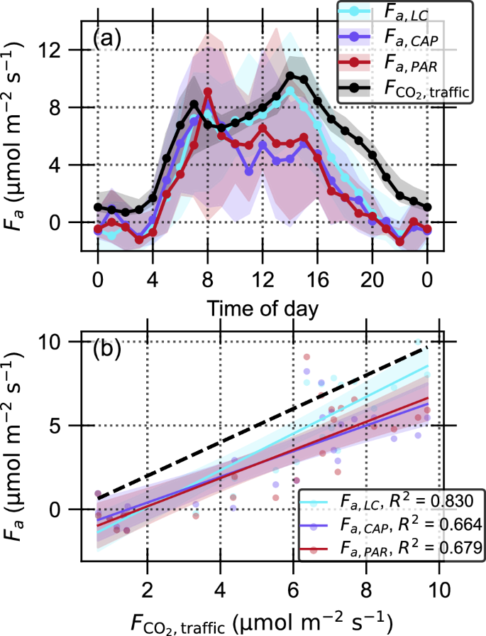
a Median diurnal cycle obtained with different methods (LC, CAP, PAR) and an independent bottom-up fossil fuel estimate (({F}_{{{rm{CO}}}_{2,{rm{traffic}}}})). Shadowed areas indicate the interquartile ranges. b Comparison of half-hourly estimates by different methods against (({F}_{{{rm{CO}}}_{2,{rm{traffic}}}})). The solid lines show the fits, shaded area the 95% confidence intervals, and the dashed line 1:1 ratio.
The COS-based CAP and PAR methods have R2 values of 0.66 and 0.68, respectively. The lower GPP values during the afternoon hours (Fig. 2) when compared to GPPLC translates into lower afternoon Fa as it is obtained as a residual from GPP and R. An additive part of the discrepancy can derive from the accumulation of error: Initial signal of high-frequency ({X}_{{rm{COS}}}) measurements has a lot of noise by default, which affects the quality of the flux calculated with the EC technique. The random errors of CO2 fluxes can vary between 10–30%36 but are even 35% for COS fluxes37. Looking at the big picture, however, COS methods succeed qualitatively in producing diurnal dynamics of Fa and a relatively good correlation, which is encouraging. If Fa,LC is considered the desired output, then CAP and PAR both produce credible results, even though the daily sums of emissions for Fa,PAR and Fa,CAP are 24% and 21% lower than that of Fa,LC, respectively.
Long-term variability
All methods catch the variability of the anthropogenic (traffic in our case) CO2 emissions and GPP during the measurement period (Fig. 4). ({F}_{{{rm{CO}}}_{2,{rm{traffic}}}}) in the street sector, it varies little over the measurement period, remaining between 6.9 and 8.4 μmol m−2 s−1. As with the diurnal variability, Fa obtained with different methods yields mostly lower estimates than obtained with the bottom-up approach. Fa,LC is, on average, the closest to ({F}_{{{rm{CO}}}_{2,{rm{traffic}}}}) (3.1–10.9 μmol m−2 s−1), while COS based methods yield mostly notably lower estimates (Fa,CAP: −1.1 to 10.3 μmol m−2 s−1, Fa,PAR: 0.6–9.6 μmol m−2 s−1). Performance of COS-based methods improves notably when the amount of available data from street sector increases. Part of Fa,LC’s success comes from the fact that parameterizations always ignore a significant amount of variability, which is detected in the COS flux-based methodology. However, the results encourage the use of light response curves where applicable.
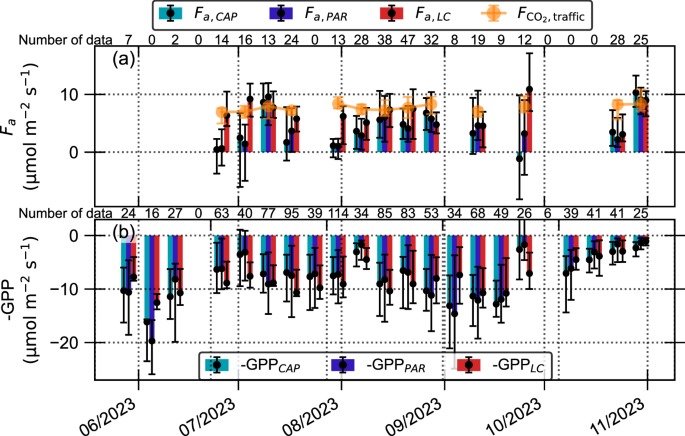
Panel (a) shows Fa at the street sector and panel (b) shows GPP from both the vegetation and the street sectors. Night-time data (PAR < 10 μmol m−2 s−1) are omitted. Bins show the median value from 10-day periods, and the whiskers indicate the interquartile range. Orange data with error bars on panel (a) show the median and interquartile range of the bottom-up estimate of fossil fuel emissions on the street sector. It is generalized into the vegetation sector by normalizing values according to the paved land surface area. The number of accepted data points for each group of bins is shown on top of the panels, and only those times with more than 10 points were plotted.
The seasonal dynamics of GPP (Fig. 4b) reflect variations in environmental conditions that the different methods are able to catch. After the driest and hottest period at the end of June (Fig. S7), there is a clear dip in the magnitude of GPP. The cloudy and rainy start of August shows a clear decrease in biogenic activity. During October, the vegetation prepares for winter dormancy, and the photosynthesis ceases completely. Finally, different methods converge towards each other: GPP approaches zero regardless of the method, thus Fa approaches R—NEE. The last week of the campaign shows an increase in all Fa’s without a significant increase in data availability. This suggests that as the temperatures fall closer to 0 °C, it becomes more likely that there are anthropogenic CO2 emissions from also other than vehicular sources. GPPLC, the most accurate on Fa, shows the least variability with the average observed CO2 uptake of 7.9 μmol m−2 s−1. COS flux-based methods are, as expected, similar to each other, but GPPPAR shows larger variability both between and within the weeks. GPPCAP yields the lowest average CO2 uptake, but a relatively high reactivity to the environmental conditions, shown as a higher standard deviation than GPPLC.
In summary, we demonstrated that COS fluxes can be used to give realistic measurement-based estimates of urban ecosystem level GPP both on diurnal and season scales. The obtained GPP values can be used together with the estimation of ecosystem respiration to estimate anthropogenic emissions within the source area of the EC measurements. Compared to light-response curves COS-based methods need a lower fraction of green area and are not dependent on an NEE measurement of purely biogenic origin, thus being a better fit for the urban environment. Nonetheless, the light-response curve of GPP remains a useful and more accurate tool in the areas where a reasonable parameterization is possible. We also acknowledge that the COS methodology might not be applicable in environments with high anthropogenic influence. However, in the areas, where the fraction of vegetated areas is large, COS flux measurements can provide useful insights to estimate the magnitude of CO2 uptake within the footprint.
Future research on urban COS exchange should consider conducting EC and chamber measurements using both shoot and soil chambers in urban vegetation to obtain a more detailed picture of the COS and CO2 fluxes along the ecosystem scale. Furthermore, COS-based GPP methodologies should be compared with other methodologies, such as remote-sensed solar-induced chlorophyll fluorescence (SIF). By expanding the methodology to other urban areas also the global COS budget closure could be further enhanced.
Methods
Measurement setup
Eddy covariance (EC) measurements were conducted on top of a 31 m high measurement tower located at the SMEAR III (Station for Measuring Ecosystem–Atmosphere Relationships38) in Helsinki, Finland (60°12’N, 24°58’E, 26 m above sea level). The station serves as an ICOS ecosystem associate site (FI-Kmp). The continuous measurement setup consisted of a uSonic-3 Scientific sonic anemometer (Metek GmbH, Elmshorn, Germany) to measure three-dimensional wind components and an enclosed path infrared gas analyzer (LI-7200RS, LI-COR, Lincoln, NE, USA), the standardized device for ICOS to measure CO2 and water vapor molar fractions39. These continuous measurements were complemented with an Aerodyne QCL gas analyzer (AD-QCL; Aerodyne Research Inc., Billerica, MA, USA) between 12 May and 31 October 2023 to measure the molar fractions of CO, COS, CO2, and water vapor. Sample air was drawn to the base of the tower through a 40 m long PTFE tubing (8 mm i.d., 22 l min−1), from where a sub-flow of 7.5 l min−1 was guided to the instrument through 4 m long PTFE tubing (4 mm i.d.) All measurements were made at 10 Hz frequency. COS concentration was calibrated daily against the NOAA-2004 scale (474.2 ppt) every 24 h. The device’s drift was corrected by employing nitrogen as a background measurement every three hours. Auxiliary environmental measurements are described in Supporting Information (SI).
Flux processing
The vertical wind and trace gas molar fractions were utilized to compute 30-min average fluxes. The process involved despiking, linear detrending and 2-dimensional coordinate rotation, following standard EC processing approaches40,41. The fluxes were computed utilizing the maximum covariance method where the time lag of CO2 was used for COS due to the noisy COS signal37. The obtained fluxes underwent spectral and storage corrections, which are described in SI. The co-spectra of COS with vertical wind exhibited a distinctive shape for the highest frequencies (Fig. S8), and the spectral correction of CO2 was thus utilized. Storage flux below the measurement height was derived by assuming a uniform concentration change through the profile for each gas (Fig. S9)37,42,43,44. To ensure the quality of the flux data, the following criteria were applied: flux stationarity <60%, kurtosis of the observation distribution between 1 and 8, and skewness between −2 and 2. Additionally, u* filtering, with a threshold set at u* = 0.19 m s−1, was employed to eliminate the impact of low-turbulence situations43. Quality control was passed by 37.9%, 59.6%, and 45.9% of COS, CO2, and CO fluxes, respectively. The relatively high omission percentage for COS fluxes was anticipated, primarily attributed to a low signal-to-noise ratio resulting from the inherently low atmospheric molar fraction of COS. Previous studies in forest ecosystems have utilized 34%18 and 48%37 of all COS flux data. The time series of fluxes that passed the quality filter are illustrated in Fig. S2. A comparison between AD-QCL and LI-7200 latent heat (LE) and CO2 fluxes exhibited a good agreement (R2 = 0.83 and R2 = 0.69), with AD-QCL yielding 14% larger and 5.4% smaller flux values, respectively (Fig. S10). Data were not gap-filled due to the heterogeneous nature of the site, and as gap-filling can bring uncertainty to the analysis45.
Ecosystem-scale urban CO2 exchange
The footprint area of the EC setup was divided into three sectors (Fig. S1), of which street and vegetation were used in this analysis as the wind direction was seldom from the built sector. The vegetation sector had 80% green land cover, whereas the street sector had almost equal amounts of paved (41%) and vegetated (46%) surfaces (Table S1). The major difference between these two sectors is the amount of human activity. The vegetation sector houses a botanical garden, an allotment garden, and recreational green spaces, while one of the busiest access roads of Helsinki city center passes the street sector. Over the study period, the road had an average traffic count of 23,400 vehicles per day as measured by the City of Helsinki traffic counter located 350 m south of the EC tower.
The urban ecosystem- or local-scale net exchange of CO2 (NEE, in μmol m−2 s−1) as measured using the EC technique can be described using a simplified equation
where R is the combined vegetation and soil respiration, GPP is the amount of photosynthetic uptake of CO2, and Fa combines all the anthropogenic sources of CO2 within the footprint area. R can be further divided into autotrophic and heterotrophic respirations, i.e., natural CO2 release from plants and heterotrophic activity, such as soil microbial decomposition, and the Fa into emissions from human respiration, building heating, and transportation8. In the vicinity of SMEAR III, however, transportation is by far the largest anthropogenic CO2 source, as building emissions take place elsewhere due to district heating, and human respiration is also modest compared to traffic35. Thus, Fa is considered synonymous with traffic emissions, keeping in mind the consequent uncertainty. To separate Fa, which is commonly the interest of urban observations, from the other components, estimations for R and GPP are needed.
A commonly used practice is to estimate R using an exponential function on temperature:
where RC is the base level of respiration, Q10 describes the increase of R when temperature increases by 10 °C, and Tsa is the driving temperature of the respiration. Following14, a half-hourly average of 10 cm soil temperature from the botanical garden and 16 m air temperature from the EC tower was used. Parameters were obtained by fitting night-time (PAR < 10μmol m−2 s−1) NEE data from the vegetation sector (Fig. S11), which is a common practice when estimating R on vegetated ecosystems46. More information about the parameterization is available in SI.
GPP methods
The photosynthetic carbon uptake of urban green areas was estimated using four different methods, with two relying on COS flux measurements. To estimate GPP from ecosystem-scale fluxes of COS (({F}_{{rm{COS}}})), a leaf relative uptake (LRU) of COS and CO2 was used12,14,47, as follows:
where ({X}_{{{rm{CO}}}_{2}}) and ({X}_{{rm{COS}}}) are molar fractions (shown in Fig. S12). In essence, LRU describes the ratio of the COS and CO2 fluxes normalized with their molar fractions. Originally, LRU was considered as a constant11,12, but later studies have shown the importance of the diurnal dynamics of LRU13,14. Ideally, LRU is measured independently using leaf chamber measurements of COS and CO2 to get a sturdy estimate for it. However, chamber measurements are often neither feasible nor representative, which presents a challenge, particularly in urban green areas with highly diverse plant species. We tested two different means to parameterize LRU on an ecosystem scale (see below).
GPPPAR from COS flux and light response of LRU
An earlier study made an LRU parameterization based on chamber measurements in Hyytiälä forest station13. It represents the LRU of the top canopy of a boreal Pinus sylvestris forest as a function of PAR following
An earlier study observed no significant differences between the LRU values of coniferous and broad-leaved tree species31. Furthermore, it has been shown that LRU is relatively invariant within the boreal biome32. Hence, the method is used here as an approximation for the diverse footprint area with predominantly broad-leaved trees and managed urban grasslands. LRUPAR was used in (3) to obtain GPPPAR in both the vegetation and street sectors.
GPPCAP from COS flux and environmental parameterization
GPPCAP is based on the CAP (carboxylation capacity) stomatal conductance optimization model14,48. Besides PAR, it takes into account more environmental variables relevant for LRU, such as VPD, SWC, and leaf area index (LAI) following
It is, in principle, universal, although applying it on different sites requires good availability of environmental parameters. The list of variables and parameters and their source is shown in Table S3. LRUCAP is used in Eq. (3) to obtain GPPCAP in both urban and street sectors.
GPPLC from an ecosystem-scale light response curve
GPPLC utilizes a form of saturating light response curve also originally used on forest ecosystems. The formulation was taken from a subarctic boreal forest as46
where α is the quantum yield, or the initial slope of the light response curve, I denotes PAR, Pmax light-saturated rate of GPP, and θ is a curvature parameter. The temperature response of photosynthesis (f(Ta)) is taken into account as
where Ta is air temperature at 16 m, and T0 = −2 °C is the inflection point. Parameters were fitted as described in SI (Fig. S11). GPPLC was then calculated for both vegetation and road sectors using the fitted parameters.
GPPEC from traditional CO2 flux partitioning
GPPEC was employed in a “traditional” manner to distinguish carbon exchange components in vegetated ecosystems where it is estimated as a residual from NEE measured using EC and R(2), as follows:
In this study, the method was primarily utilized for comparison to the other methods and secondarily to demonstrate its incompatibility in areas where anthropogenic CO2 emissions become non-negligible.
Traffic emissions
To assess the accuracy of the final anthropogenic emissions obtained with different GPP estimates, we compare the flux-derived estimates against bottom-up estimates of fossil fuel emissions originating from vehicular transportation in the street sector (({F}_{{{rm{CO}}}_{2,{rm{traffic}}}})). Estimates of Fa were only made for the street sector because human activities in the vegetation sector were small. Also, we only consider Fa estimates just by LC, CAP, and PAR methods as for EC method Fa is trivially zero. The traffic rate measured at the access road by the City of Helsinki was combined with weighted unit emission factors (EF) obtained from The Handbook of Emission Factors for Road Transport (HBEFA)49. EFs were obtained separately for different road types, each with their mean velocities matching with those obtained from the traffic counts. Velocity-dependent EF was obtained by fitting a line to the velocity-EF plane (Fig. S13b). The obtained relationship was
where V is the average speed in 30-min period in km h−1. The emission factor was multiplied by the number of cars per 30-min period and normalized by the area of paved land cover on the street sector to obtain the final vehicular CO2 emission. The emission factors on the velocity range from 30 to 70 km h−1 were considered trustworthy with this methodology. Earlier modeling from the area in 2012 estimated EF of 298 gCO2 km−1 car−1 35, which is considerably higher than ours (183 ± 7 gCO2 km−1 car−1). This can be partly accounted for the development of cars and the slowly increasing fraction of electronic vehicles and partly for the different methodologies used.
The real CO2 signal originating from the street sector gets diluted on its path to the EC setup depending on the prevailing wind direction and the distance to the street. To account for this, an artificial dilution was added to the ({F}_{{{rm{CO}}}_{2,{rm{traffic}}}}) estimate. This was achieved by dividing the street sector into 20° slices with radii of 350 m (distance to the traffic counter, see Fig. S1), and weighting each estimate with a factor
where pslice is the paved fraction in each slice and pslice,max is the highest paved fraction across all slices. Thus, ({F}_{{{rm{CO}}}_{2,{{traffic}}}}) was weighted for every timestep with a factor ranging between 0–1 depending on the average wind direction during the 30-min period.

Responses