Dynamic configuration before quasi-biennial oscillation disruptions revealed from the perspective of planetary waves

Introduction
The zonal wind field in the stratosphere over the equatorial region propagates downward and alternates from easterly wind to westerly wind with an average period of 28 months, which is called quasi-biennial oscillation (QBO). The QBO was first detected by Ebdon1 and Reed2, and the current consensus is that the multi-scale wave modes driving the QBO include Kelvin, Rossby, mixed Rossby-gravity, inertia-gravity, and small-scale gravity waves3,4,5,6,7,8,9,10. QBO is closely related to climate change and ecological environment, and its predictability also provides convenience for related research11,12,13,14,15,16.
From December 2015 to March 2016, the westerly phase of QBO has been interrupted abnormally for the first time since 1953, with easterly winds appearing near 40 hPa and an upward displacement of westerly winds near 20 hPa17,18. This is known as the 2015/16 QBO disruption (2015/16D). This anomaly is believed to be related to the enhanced westward momentum carried by an equatorward-propagating Rossby wave originating from the Northern Hemisphere17,18,19,20. Surprisingly, a second abnormal disruption occurred only a few years later during June–September 2019 (2019/20D). Kang and Chun21 conducted a detailed analysis of various equatorial planetary waves (PWs) and parameterized gravity waves in the 2019/20D, and compared them with the 2015/16D22. The results showed that the intense PW activity in 2019/20D may have been related to a minor sudden stratospheric warming (SSW) in the Southern Hemisphere in September 201923. External forces that caused abnormal atmospheric circulation in the stratosphere over the equator mainly came from the meridional propagating PWs from the Northern and Southern Hemispheres respectively, accompanied by meridional momentum flux stronger than the climatology24. The above results provide us with a deeper understanding of the planetary-scale wave activity behind the two QBO disruption events.
Although previous studies showed that PWs accompanied by strong momentum forcing from the mid-latitudes contribute significantly to the two QBO disruptions, the propagation and dissipation process of the PW and specific wave-mean flow interaction mechanism throughout the whole stratosphere are still open questions. Besides, the 2010/11 winter (the identification of winter and summer is based on the Northern hemisphere) also provides comparable wave momentum flux divergence in the equatorial region18 with strong meridional EP flux (Table 1), but lacks the zonal wind reversals, indicating some differences in wave propagation process. Our study aims to discuss these issues.
Results
PW characteristics during the two events compared to climatology
To obtain an intuitive impression of the PW activity during the two QBO disruptions, the differences between them and the climatology for the corresponding period are compared here (Fig. 1). The wave parameters on 46 hPa and 10 hPa pressure layers are calculated here from MLS data (method) for comparison, since the anomalous westerlies appear to curtail the easterly phase downward propagation at 10 hPa and anomalous easterlies develop within the westerly phase at 40 hPa24,25.

Latitudinal cross-section of PW amplitude at (a, b) 46 hPa and (c, d) 10 hPa, zonal mean zonal wind at (e, f) 46 hPa and (g, h) 10 hPa, meridional EP flux of zonal wave numbers 1–3 at (i, j) 46 hPa and (k, l) 10 hPa and EP flux divergence of zonal wave numbers 1–3 at (m, n) 46 hPa and (o, p) 10 hPa, taking time average of December–March in the Northern Hemisphere (left half of panel: a, c, e, g, i, k, m, o) and June–September in the Southern Hemisphere (right half of panel: b, d, f, h, j, l, n, p) from 2004 to 2022. The black lines represent 2015/16D and 2019/20D, respectively. The blue lines represent the 2010/11 winter. The climatology (red lines) is overlaid with the ±1 standard deviation (red shading). Locally enlarged subgraphs containing data at the four lowest latitudes are supplemented to make the distribution of low latitudes more distinguishable (for the amplitude, these are 2.5°N/°S, 7.5°N/°S, 12.5°N/°S, and 17.5°N/°S; for the EP flux divergence, these are 17.5°N/°S, 22.5°N/°S, 27.5°N/°S, and 32.5°N/°S).
The MERRA2 reanalysis data also obtained almost the same results as Fig. 1 (Fig. S1). Considering that the magnitude of the wave parameter changes significantly with the decrease of latitude, the corresponding local magnifications are also drawn in the subplots of amplitude and EPFD (containing data at the four lowest latitudes) for easy identification. Compared with climatology, relatively strong wave amplitudes (close to or exceed one standard deviation) appear at both 10 hPa and 46 hPa in mid latitudes (40°N–60°N/40°S–60°S) during the two QBO disruption events. In low latitudes (17.5°N–22.5°N/17.5°S–22.5°S), the zonal wind is more positive (stronger westerly wind) at 46 hPa while more negative at 10 hPa than climatology. The meridional EPF at 46 hPa is significantly stronger than the mean value at low latitudes (17.5°N–22.5°N/17.5°S–22.5°S), indicating that the equatorward-propagating PWs in the subtropics are more conducive to penetrating the tropics at 46 hPa. The meridional EPF is not prominent at 10 hPa, this is because a four-month climate average masks some of the strong transmissions (Fig. S2 shows more intense wave transmission over a shorter time average). During the westerly QBO phase in the 2010/11 winter, the wave amplitudes are relatively strong at high latitudes (60°N–80°N/60°S–80°S) at both 10 hPa and 46 hPa, while at low latitudes, they are also larger than that of 2015/16D. At 10 hPa, the wave amplitudes stronger than climatology at high latitudes during 2015/16D and 2019/20D all become smaller than climatology at low latitudes. Notably, this change is not observed for the 2010/11 winter. Thus, we hypothesize that in addition to the normal dissipation process during the equatorward propagation of the PW, there may be other mechanisms that accelerate the decline of the wave amplitude and produce additional forcing to the mean flow, which may also be connected to the formation of QBO disruptions. In other words, it is possible that in addition to the forcing effect of PW in the lower stratosphere on the QBO disruptions, which has been emphasized by existing studies, there are still important PW effects in the middle stratosphere that have not been paid attention to, and this can explain the absence of QBO disruption in 2010/11 winter.
Abnormally low correlation coefficient
In searching for this additional wave forcing, the Pearson correlation coefficients of PW amplitudes sequences at two adjacent latitudes is calculated during corresponding period through the entire pressure layers. When calculating the PW amplitudes sequences, 2.5°N/°S, 7.5°N/°S, …, 77.5°N/°S, and 82.5°N/°S are taken as the central latitude, with 2.5° expanding to the south and north, respectively. Then the time series at a certain latitude is obtained after meridional average (December–March for the Northern Hemisphere and June–September for the Southern Hemisphere), and the correlation coefficients are calculated at 0°N/°S, 5°N/°S, …, 75°N/°S and 80°N/°S, respectively. Although the wave amplitudes decrease rapidly as the latitude decreases, the time series of PW amplitudes at adjacent latitudes tend to have similar variation trend when there is no external force. However, when there is a correlation coefficient that deviates significantly from the climatology, it can be considered that additional forcing or dissipation occurs at nearby latitudes, causing significant changes in PW activity. Here the time-longitude cross-section of geopotential height (GPH) anomalies is used to see features of the PW appearance, as well as the zonal movement (eastward, westward, or quasi-stationary) of the main wave components26.
Figure 2a, b shows the correlation coefficient of time series of PW amplitude between adjacent latitudes, with a value between 0 and 1. Abnormally low correlation coefficient can be seen at 10 hPa during 2015/16D and 8 hPa during 2019/20D. Of course, this low value also exists in the adjacent pressure layers (Fig. S3). For brevity, only the pressure layer with the most obvious deviation of the correlation coefficient from climatology is shown here. For the latitudes corresponding to the abnormally low correlation coefficient (27.5°N and 22.5°N for 2015/16D, 17.5°S and 12.5°S for 2019/20D), the time-longitude sections of the GPH anomalies on the corresponding pressure layers are plotted to show the anomalous PW activity (Fig. 2c–f). The two sections are selected here because the abnormal low value of the correlation coefficient means the significant difference between the two PW amplitudes sequences at the adjacent latitudes, which can be worth further exploring the additional forcing or dissipation effects of PWs behind it. In 2015/16D at 10 hPa, there are three obvious eastward-propagating waves (marked as wave a, wave b, and wave c), accompanied by significantly dissipation (the disappearance of a distinct signal of eastward-propagating waves) during the equatorward-propagation. Mutations of these three waves have led to significant changes in the trend of the PW amplitude sequence. In 2019/20D, there are two obvious eastward-moving waves (marked as wave d and wave e) at 17.5°S (8 hPa), which gradually disappear at 12.5°S. According to linear wave theory, equatorward-propagating PWs will dissipate nearby when they encounter critical latitudes, where the zonal wind matches the wave phase velocity27,28. These additional dissipated eastward-propagating waves happen to correspond to the enhanced easterly wind in the middle stratosphere, which means that it is more conducive to the period when subtropical PWs affect the equatorial QBO.
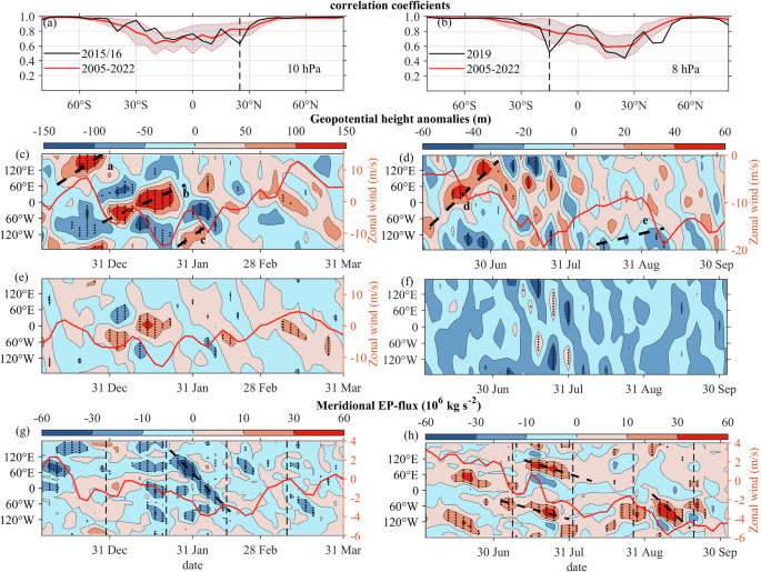
Top panels: correlation coefficients of PW amplitudes during corresponding period between adjacent latitudes at (a) 10 hPa during 2015/16D, and (b) 8 hPa during 2019/20D; Middle Panels: time-longitude sections of GPH anomalies at 10 hPa at (c) 27.5°N, and (e) 22.5°N during 2015/16D and GPH anomalies at 8 hPa at (d) 17.5°S, and (f) 12.5°S during 2019/20D; Bottom panels: time-longitude sections of 38 hPa meridional EP flux (g) at 17.5°N during 2015/16D, and (h) at 17.5°S during 2019/20D. The periods for subsequent analysis are bracketed by vertical dashed black lines in (g, h). The red curves superimposed on (c–e) and (g, h) represent the zonal mean zonal wind at the corresponding pressure levels. The black dots indicate where the anomalies are more than one standard deviation above the climatology in (c–h).
The results in Fig. 2 can also be reproduced by MERRA2 data (Fig. S4). Here the wave packet is indicated by the meridional EPF, similar to the previous studies using the maximum value of the disturbance29,30. It should be noted that near the equator, the correlation coefficient of the wave amplitude series on the adjacent latitudes of the MLS data is low (Fig. 2a, b), while that on the adjacent latitudes of the MERRA2 data is high (Figs. S3a, b). This is because the calculation of the wave amplitude comes from the zonal distribution of the GPH, and this distribution has uncertainties within 7.5°S–7.5°N for results from MLS and MERRA2 data due to potential discrepancies in geopotential height (Fig. S5). Therefore, the abnormally low correlation coefficient during the two QBO disruption events are credible and reasonable, eliminating the interference with data quality.
Strong westward-moving wave packets in the lower stratosphere
To quantify PWs entering the equatorial region from mid-latitudes, time-longitude sections of the meridional EPF during 2015/16D and 2019/20D are plotted in Fig. 2g, h, respectively. Wave packets that have significant GPH anomalies (1 standard deviation above climatology) and move westward are marked with bold black dashed lines, indicating strong westward-propagating wave packets. In late January of 2015/16D, a strong equatorward-propagating wave packet appeared (Fig. 2g), with a westward phase velocity of approximately 10.5 m/s (obtained from the slope of the wave center axis). Coincidentally, a westward-moving wave packet with a phase velocity of 12 m/s has already been found at 4.5°N during a similar period, which finally caused the drastic deceleration of the equatorial jet31. It can be assumed here that this was probably the same wave packet that originated from the mid-latitudes. As for 2019/20D (Fig. 2h), three strong westward-moving wave packets (three black dashed lines) occurred, among which the strongest wave packet occurred in September. Based on ERA5 reanalysis24, the persistent strong meridional forcing during 2019/20D covered a longer period with a maximum value in early September, while the peak forcing during 2015/16D concentrated in a shorter period and reached the maximum value in late January and early February, which is also in agreement with our results. The peak of the meridional EPF and the occurrence of the eastward-moving wave dissipation (wave b, wave c, wave d, and wave e) overlap (Fig. S6), showing the consistency and integrity of dynamics configuration in upper and lower stratosphere.
Forcing and propagation of PWs in different periods
For subsequent analysis, the vertical black dashed lines in Fig. 2g, h divide a complete period into three consecutive sub-intervals. They are T1 (December 28–January 20), T2 (January 21–February 13), and T3 (February 14–March 8) in 2015/16D, and T4 (July 7–July 30), T5 (July 31–August 23), and T6 (August 24–September 16) in 2019/20D. The latitude-height sections of the EPF and the wave-driven DF during the consecutive sub-intervals are c shown in Fig. 3. In the subsequent processing for the vertical direction (involving calculations such as derivation in the vertical direction), the original data (261 hPa~0.1 hPa, a total of 36 air pressure layers) is interpolated to the logarithmic air pressure value of equal spacing (({log }_{10}P) from 2.4 ~ -1, that is, 251 hPa~0.1 hPa, a total of 18 (P) values). For 2015/16D, when there was a strong meridional EPF in the lower stratosphere at low latitudes (T1, T2), the significant wave dissipation (dotted blue area for EPF convergence) occurred in the middle stratosphere, which did not occur in T3. In T3 period, the equatorial propagation of PWs is significantly weakened, and the meridional EPF at low latitudes also becomes much smaller. During 2019/20D, the meridional EPF in the lower stratosphere is stronger in T4 and T6 compared with that in T5, while in the middle stratosphere, the wave dissipation became strongest in T6, with significantly enhanced equatorward-propagation of PWs from middle latitudes. In the middle stratosphere (near 10 hPa), there are enhanced easterly winds during T1 and T2 for 2015/16D, and during T3 for 2019D, which facilitates the eastward propagation of PWs in the middle stratosphere from mid-latitudes to the equator.
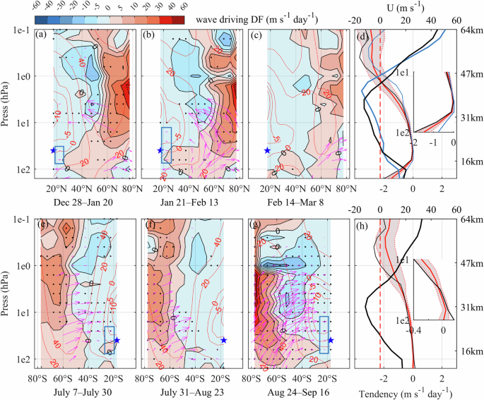
The latitude-height section of wave-driven DF (color shading) and EP flux F (vector) in (a) T1, (b) T2, and (c) T3 during 2015/16D, and (e) T4, (f) T5, and (g) T6 during 2019/20D; Meridional EP flux divergence at (d) 17.5°N during 2015/16D and (h) 17.5°S during 2019/20D. The red curve and shading represent climatology and ±1 standard deviation, respectively; the thin black lines and thick black lines represent meridional EP flux divergence and zonal-mean zonal wind in 2015/16D and 2019/20D, respectively. The blue stars represent the location of the 38 hPa pressure level at 17.5°N (17.5°S). The blue thick solid line and the blue thin solid line in (d) represent the average zonal wind and the EP flux divergence in the winter of 2010/11, respectively. In (a−c and e−g), the black dots indicate where the wave-driven DF are statistically significant (one standard deviation above the climatology), and vector arrows indicating a significant EP flux are also retained. The blue rectangular box marks the area where the EP flux is significant near the equator (17.5°S and 17.5°N), which means the strong equatorward-propagation of PWs.
The vertical profiles of the mean meridional EPFD in 2015/16D and 2019/20D are plotted in Fig. 3d, h, respectively (black curve), and the 2010/11 winter is also drawn for comparison (blue curve). The meridional forcing trend due to meridional EP-flux convergence between 40 hPa and 100 hPa in 2015/16D is extremely strong, with one standard deviation higher than the climatology (17.5°N), while the meridional forcing in 2019/20D is more negative in the middle stratosphere (17.5°S). Besides, the vertical distribution of meridional EPFD calculated from MLS data during the two QBO disruptions events seems to have a similar vertical distribution of meridional EPFD with the results obtained from the ERA5 data24, which increases the credibility and rationality of the results.
Coy et al. 18 conducted a detailed analysis of the link between the 2015/16D and equatorial wave activity using MERRA2 data. They mentioned that although the 2010/11 winter had a stronger momentum flux divergence in the equatorial region than the 2015/16 winter in the tropical lower stratosphere, there is no zonal wind reversal for the former. Figure 3d may provide a reference for clarifying this phenomenon. Within 40–100 hPa, the meridional forcing due to PWs is significantly weaker in the 2010/11 winter (blue curve), while in 2015/16D, it deviates significantly from climatology (black curve). During the two QBO disruptions, accompanied by the strong westward-propagating wave packets in the lower stratosphere, breaking of eastward-moving waves also occurred in the middle stratosphere, with enhanced meridional forcing trend (Fig. S6). Besides, the propagation and dissipation of PWs in the corresponding periods calculated from MERRA2 data show the consistent feature, whether based on the geostorophic zonal wind (Fig. S7) or the measured zonal wind (Fig. S8). For 2015/16D, from 0° to 17.5°N during T1 and T2, the meridional propagation of PW is still strong at 40 hPa, with significant negative forcing, meaning that the influence of wave dissipation from the extra-equatorial region can enter the equatorial region, and the similar result was found in 2019/20D during T4 and T6 (Fig. S8).
Breaking up of eastward-moving waves
To further demonstrate the breaking of eastward-moving waves, the variation of the longitude-height section of GPH anomalies with time is plotted in Fig. 4. Here a wave breaking is identified as the more dispersed GPH anomalies than before (more fragmented), with reduced amplitude. The time-height sections of temperature at 77.5°N (77.5°S) and meridional EPF at 17.5°N (17.5°S) in 2015/16D (2019/20D) are plotted on the right column. The variation of phase with height (the phase contour decreases with height, indicating that the wave is propagating upward) is used to obtain the vertical propagation direction of the wave, and the variation of wave amplitude of zonal wave number 1 (wave 1) and zonal wave number 2 (wave 2) is used to further illustrate wave breaking (Fig. S9). For 2015/16D, the strong meridional EPF at 38 hPa was mainly concentrated in late January and early February. In early February, when there was a strong wave packet in the lower stratosphere (Fig. 2g), there was a strong wave dissipation in the middle stratosphere, accompanied by the breaking of an eastward-moving wave and the strengthening of negative forcing (Fig. S6). From January 28 to January 31, wave 2 at 1 hPa was gradually replaced by wave 1 with a stronger amplitude. Then the strong wave 1 perturbation extended downward (Fig. S10) and moved westward until February 12. During this period, the amplitude of wave 1 weakened, while the amplitude of wave 2 increased. For 2019/20D, strong wave packets at 38 hPa exist in both July and September, but there are stronger equatorward-propagating PWs and wider wave dissipation in the middle stratosphere in September (Fig. 3g). From September 14 to September 17, wave 2 at 1 hPa is gradually replaced by wave 1, with an enhanced amplitude and downward extension of the perturbation. Significant wave dissipation is seen after September 14 (Fig. 4), close to the period with enhanced negative forcing (Fig. S6). In both disruptions, the vacillations of amplitude between wave 1 and wave 2 reflect wave-wave interactions in the stratosphere32,33. Although a single pressure layer (38 hPa) is selected here to identify the characteristics of wave packets, it can be seen from both the MLS data-based results and MERRA2 data-based results (Fig. S10) that the strong wave packets prompting the zonal wind reversal existed in the wider stratosphere. In 2015/16D, one strong wave packet mainly occurred in early February and between pressure layers of 56 hPa and 31 hPa (red rectangular). In 2019/20D, two strong wave packets occurred in late July and between pressure layers of 46 hPa and 24 hPa, while one strong wave packet occurred in early September and between pressure layers of 40 hPa and 10 hPa (red rectangulars), respectively. Other scattered but still marginally strong wave packets are not discussed here, which may also contribute to the appearance easterly wind with still relatively strong westward forcing.
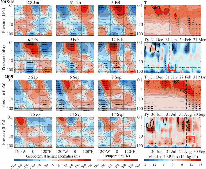
Right column: Time-height section of temperature T at 77.5°N (77.5°S) and the meridional EP flux Fy at 17.5°N (17.5°S) during the 2015/16D (2019/20D) events. The black vertical lines represent the period from January 28 to February 12 and from September 2 to September 17, respectively. The dashed red line corresponds to the 38 hPa pressure layer, and the solid black line represents the contour with the meridional forcing of −5 m s–1 day–1. The left three columns are the longitude-height sections of the GPH anomalies at 17.5°N (17.5°S), corresponding to the time interval bounded by black dotted lines in the panels on the right column. The black dots indicate where the results are statistically significant (one standard deviation above the climatology).
The PW activity behind the two QBO disruptions is likely to be closely related to SSW (the sudden increase and transfer to the lower altitudes in temperature in Fig. 4), as the wave packets in early February during 2015/16D and early September during 2019/20D appear almost simultaneously with the major SSW in 201634,35 and the minor SSW in 2019, respectively23,36,37. When the strong meridional wave packets appear, the amplitude of waves 1 and 2 at 17.5°N (17.5°S) is statistically significant, corresponding to the simultaneous enhancement and downward extension of both waves in the high-latitude (62.5°N/62.5°S) stratosphere during the two SSW events (Fig. S11). The increase in PW transmission at mid-latitude is also related to the increase in PW transmission at lower latitudes (Fig.3 and Fig. S2). Li20 has found interactions between the quasi-stationary wave 1 and faster wave 2 around 15°N during 2015/16D, which may provide the largest horizontal momentum deviation. In both disruptions, the interaction of the eastward-moving wave with the downward-propagating WN1 PWs above (phase tilts eastward with altitude in Fig. S12) that provides the additional negative forcing to reverse the zonal wind. The locally generated downward-propagating WN1 PWs occurs in the westerly wind phase of the stratopause and is hardly affected by the QBO below38. Previous research has shown that the occurrence of SSWs favors upward eastward-propagating PW activity from the lower stratosphere39,40, which also supports our conclusion.
In order to prove that the remaining eastward-moving waves after dissipation near 20o N/S influence QBODs near equator, the distribution of EP flux divergence during the corresponding period at different latitudes is shown in Fig. 5. With the decrease of latitude, it can be seen that the height of EP flux divergence that significantly exceeds the climatology gradually decreases from 6 hPa to 40 hPa, showing that the gradual downward effect of wave forcing is continuous as the latitude decreases. During the period of dissipation of the eastward-moving wave (January in 2015/16D, June and early September in 2019/20D), strong negative forcing in the middle stratosphere over extra-equatorial region (17.5° N/S) can be extended to the equatorial region (7.5° N/S) in the lower stratosphere in the immediate subsequent period (Fig. S13). The results wellreflect that the eastward-moving wave dissipation in the middle stratosphere over the extra-equatorial region can affect the lower stratosphere in the equatorial region, and the time period exactly corresponds to the wave packet dissipation in the middle stratosphere and the strong wave transmission in the lower stratosphere in Fig. 2.
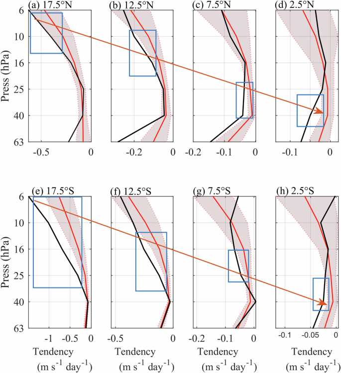
EP flux divergence at (a) 17.5°N, (b) 12.5°N, (c) 7.5°N, and (d) 2.5°N, during 2015/16D and (e) 17.5°S, (f) 12.5°S, (g) 7.5°S, and (h) 2.5°S during 2019/20D. The red curve and shading represent climatology and ±1 standard deviation, respectively; the thin black lines represent EP flux divergence in 2015/16D and 2019/20D, respectively; the rectangular box marks the significantly enhanced negative forcing.
Verify the dynamical configuration through all years
A previous study noted that strong westerly winds in the equatorial lower stratosphere provide favorable conditions for QBO disruptions by hindering the wind reversal at its base, making it easier for westerly equatorial waves to propagate upward above 70 hPa41. We further illustrate the connection between wind field and wave activity by plotting the difference between two QBO disruption events and the climatology during consecutive periods (Fig. 6). Compared with the whole period (Fig. S14, from December to March for 2015/16D and from June to September for 2019/20D), the results in Fig. 6 are subdivided into shorter periods to avoid short-term wind field changes being masked by seasonal averages. In the lower stratosphere, there is an accelerated westerly jet, consistent with Kang’s results41, in both the entire disruption period and the four divided periods. This emphasized such a causal line for the wind field and PWs in the lower stratosphere: the equatorial westerly acceleration in the lower stratosphere → the increase of westward tropical PWs propagating upward → enhanced westward negative forcing → suppressed zonal wind field at 40 hPa.
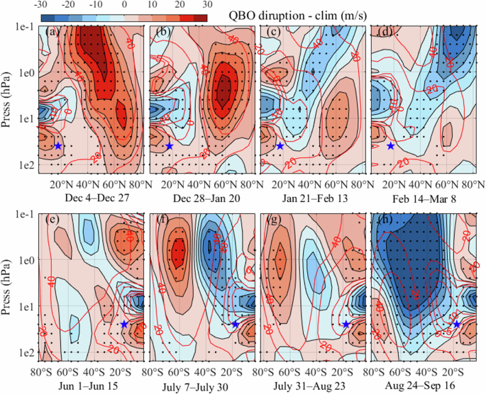
Differences in the zonal-mean zonal wind between QBO disruption and climatology for 2015/16D (a–d) and 2019/20D (e–h) in four periods. (a, e) correspond to the period before the eastward-moving wave (Fig. 2c–d), and the rest of the periods correspond to T1-T6. The blue stars represent the location of the 38 hPa pressure level at 17.5°N (17.5°S). The red contours represent the zonal mean zonal wind after the time average in the corresponding period, and the shadings represent the wind speed difference with the climatology. The black dots indicate where the results are statistically significant (one standard deviation above the climatology).
During the two complete QBO disruptions, compared with the climatology, there was a continuous strong easterly wind in the tropical middle stratosphere (near 10 hPa), which was conducive to the eastward-propagating wave packets penetrating to lower latitudes. For 2015/16D, in the early stage of the disruption (Fig. 6a, b), there was an enhancement of the westerly wind at a higher altitude above the strong easterly wind, which is conducive to the downward propagation of westward-moving 1 wave (Fig. 4) and the formation of a strong wind shear area that promotes wave breaking42. The similar wind field configuration also appeared during the early stage (Fig. 6e) and late stage of 2019/20D (Fig. 6g, h) in the tropical middle stratosphere. This wind field structure was also captured by the MLS data during the corresponding periods (Fig. S15). A causal line for the wind field and PWs in the lower stratosphere can also be revealed: the strong easterly wind in the middle stratosphere → the increase of eastward-propagating PWs penetrating to lower latitudes → enhanced wind shear in the middle stratosphere → enhanced negative forcing from the dissipated eastward-moving wave.
Take 2015/16D as an example to illustrate this mechanism (Figs. S8a–c). As the eastward wave propagate toward the equator, easterly winds below 10hPa are gradually increasing, and wind shear increases significantly (vertical distance of wind speed contour becomes narrower). From Dec 28 to Jan 20, PW in the middle stratosphere is accompanied by obvious wave dissipation during its equatorial propagation. From Jan 21 to Feb 13, in the middle stratosphere, the wave dissipation process of eastward moving ends. In the equatorial region of the lower stratosphere, there is a strong meridional wave transport, accompanied by an enhanced negative forcing. Westerly winds in the equatorial region near 40 hPa gradually change to easterly winds during this process. A similar process can be found in 2019/20D.
Through the two specific events of QBO disruptions, we found a typical configuration, combining the enhanced negative forcing in the middle stratosphere with the breaking of the eastward-moving wave and the strong westward-moving wave packets in the lower stratosphere, that led to the QBO disruptions in the tropical stratosphere. The results for all years in the MLS dataset are listed to see if this dynamic configuration only occurs in the two circulation anomalies (Table 1). The existence of anomalously low correlation coefficient can be used to determine the obvious wave breaking during the equatorward-propagation of PW. The start dates of SSW events are noted. In the winter of 2011, and in the summer of 2006, 2008, and 2013, there are also strong meridional wave propagation in the lower stratosphere (Table 1), with relatively strong westward wave packets (Fig. S16). However, QBO disruptions did not occur in these examples, this further proves that dissipated eastward-moving wave in the middle stratosphere is likely to play a key role in QBO disruptions, which has not been noticed by predecessors. Therefore, it seems that equatorward propagation of eastward-moving PWs has a cause-effect on the QBO disruptions. On the one hand, due to the wind field structure (Fig. S17), the lack of a critical line allows subtropical eastward-moving (westward-moving) waves in the middle (lower) stratosphere to affect the equatorial wind field; On the other hand, the SSW events may promote the occurrence of eastward-moving waves37,38. Both the wind and temperature structure can lead to the QBO anomaly25,41.
It should be noted that during the period of 2004–2022, there are some abnormally low coefficients in the middle stratosphere in other years (Table S1). However, eastward-moving PWs that may affect the QBO structure only occurred in Northern Hemisphere winters of 2015/16, and Southern Hemisphere winter of 2019. In the existing dataset, we once again confirm the uniqueness of the proposed dynamical configuration in identifying circulation anomalies. Since the two QBO disruptions occurred in February 2016 and December 201924, this dynamic configuration can be used as a precursor within several weeks in advance. Strong easterly winds in the middle stratosphere and enhanced westerly winds in higher altitudes at an earlier stage (before the dissipation of eastward-moving waves over the equator) also provided favorable conditions for mid-latitude wave activity to affect the stratospheric wind field over the equator. This dynamic configuration is closer in 2015/16D and farther away in 2019/20D. This is because the extratropical PWs act at different stages in the two circulation anomaly events21,22,41. Besides, the downward extension of wave signal (momentum deposition) in the middle stratosphere on seasonal time scales is closely related to the evolution of the jet stream43,44,45, and corresponds to the time advance of the dissipated eastward-moving wave packet from QBO disruptions.
Discussion
In historical observations, there has never been such stratospheric atmospheric circulation anomalies in tropics showing as the two QBO disruptions, and the time interval between them is so close. The QBO is a regular feature in the climate system with more than three years of predictability8,11. However, two disruption events have introduced challenges to climate prediction centers to correctly reproduce the QBO. Considering that most of the current circulation models that can generate a reasonable QBO use adjustable parameterizations with large uncertainties to resolve small-scale waves46, the failure of this circulation anomaly to be predicted by models is likely due to the fact that abnormal wave activity during the corresponding time period is not adequately represented. Therefore, it is necessary to fully understand the wave activity underlying the two disruption events. Since the specific forcing process on the reversal of the QBO westerly phase from the mid-latitude PWs is still unclear, we investigate the PW activities from the winter hemisphere during 2015/16D and 2019/20D, respectively.
The results showed that the PW activity behind the two disruption events was significantly stronger than climatology, and that the zonal wind at low latitudes was favorable for the equatorward propagation of PWs in the lower stratosphere. There were several single strong westward-moving wave packets in the lower stratosphere, accompanied by strong meridional momentum transport. The enhanced easterly winds in the middle stratosphere promote the eastward-moving waves (7–10 hPa) to penetrate to lower latitudes. The strong wind shear may promote the dissipation of eastward-moving waves, producing additional negative forcing on the mean flow. The influence of wave dissipation from the extra-equatorial middle stratosphere can extend to the equatorial lower stratosphere, indicating that in addition to strong westward-moving PWs from mid-latitude in the lower stratosphere, the presence of dissipated eastward-moving waves in the middle stratosphere is also indispensable for the formation of QBO disruptions.
It is crucial to maintain the robustness and stability for the prediction of QBO, in order to grasp the change trend of the relevant circulation structure in advance. Based on the analysis results of PW activity in the two disruption events and further comparison with other years, we propose a dynamic configuration that may reveal circulation anomalies from the perspective of PWs, that is, the occurrence of eastward-moving wave dissipation in the middle stratosphere and the strong equatorward-propagating wave packet moving westward in the lower stratosphere, accompanied by an enhanced negative forcing to the mean flow. The occurrence of intense wave packets coincided with the major SSW in 2016 and minor SSW in 2019, indicating a possible connection between them. Since different activity of PWs leads to discrepancy among SSWs47, the particularity of these two SSW events and the characteristics of eastward-propagating PWs prior to them worth further investigation. Considering that such anomalies are likely to increase in a changing climate15,24,48, it makes sense to use wave dynamic configuration to capture such anomalies in advance. Previous research has pointed out the stationary wave field is an important precursor to stratospheric polar vortex anomalies49, this study shows that it can also be used as a precursor to tropical stratospheric circulation anomalies. Climate simulation deserve to be further carried out to examine the variability of QBO and the dynamic configuration proposed here.
Methods
Satellite data
The observation data used in this paper is from the Earth Observation System (EOS) satellite. We selected the temperature and geopotential height (GPH) data as measured from the Aura Microwave Limb Sounder (MLS) version 4.2 from 2004 to 2022. The altitude range is from 9.4 km (261 hPa) to 97 km (0.001 hPa), covering a latitudinal range from 82°S to 82°N. Livesey50 provided a reference for a detailed data description of this instrumentation. Some filtering techniques are used here to reduce the noise interference. The original data are averaged over a cumulative five-day period since the contribution from the extratropical Rossby waves are low-frequency components30, then a 1-2-1 zonal average is performed in a grid space of 10° longitude × 5° latitude at every latitude.
Reanalysis data
The reanalysis data used in this paper is the Modern-Era Retrospective analysis for Research and Applications version 2 (MERRA2) from 2004 to 2022. The data has a time resolution of 6 h and a spatial resolution of 0.5° × 0.625°, and contains 42 pressure layers, ranging from 1000 hPa to 0.1 hPa. The data is processed in the same way as satellite data. The purpose is to compare and verify the satellite observation results from the reanalysis data.
Calculation of wave parameters
The zonal mean zonal wind (bar{{boldsymbol{u}}}), zonal wind disturbance ({{boldsymbol{u}}}^{{boldsymbol{{prime} }}}), and meridional wind disturbance ({{boldsymbol{v}}}^{{boldsymbol{{prime} }}}) can be obtained based on gradient wind balance in a spherical coordinate system ((lambda ,phi ,z)), where λ, ϕ, and z represent longitude, latitude, and a log-pressure coordinate, respectively26,51. The relevant equations are as follows:
where a, f, and Φ are the radius of the Earth, Coriolis parameters, and geopotential, respectively. The wind field calculated in this way show good consistency with the model output, verifying the reliability of this method in regions beyond the equator52. Using harmonic analysis, a spatial Fourier Transform is performed on grid data along the longitude direction at each latitude and pressure layer, then the distribution of perturbations on each latitude circle (corresponding to one value on each longitude) can be obtained, allowing to investigate large-scale wave components with zonal wave numbers from 1 to 353. Here the deviation of geopotential is a four-dimensional function of atmospheric pressure, latitude, time, and longitude, and the four-dimensional structure of the meridional EPF is further obtained. The wave amplitude for certain number is obtained by FFT transformation of the geopotential height.
The Eliassen-Palm (EP) flux, F, and wave-driven flux divergence, DF, are used as diagnostic tools for wave activity and can reflect the propagation and forcing of PWs on the zonal mean flow54. These are calculated by the following formulas:
where (theta) and ({rho }_{0}) are the potential temperature and atmospheric density, respectively. Here, the meridional EP flux (EPF) is used to describe the intensity of the equatorward horizontal transport of PWs, the EP flux divergence (EPDF) and its meridional component is used to describe the wave forcing on background flow. To ensure the effectiveness of Eq. (1) for calculating the wind field, the resultant wind speed, EP flux, and divergence in this paper are limited to 15°N–80°N and 15°S–80°S latitude range51. The parameters at a given latitude are represented by a regional average with a latitude band width of 5°. Besides, in order to carry out momentum budget analysis in the equatorial region, the measured wind field, EP flux and divergence are calculated using the measured zonal wind to compare the results with those based on geostorophic zonal wind.


Responses