A source-weighted Benthic minus Planktonic radiocarbon method for estimating pure ocean water age

Introduction
Pure water age, or the ideal age, defined as the time elapsed since the water mass leaves the surface, is an important indicator of deep ocean circulation and carbon cycle1,2. An accurate estimation of pure water age from ocean observations, however, remains challenging. Radiocarbon (({14atop}C) has been considered one of the most promising proxies for estimating the pure water age. This is because radiocarbon (({14atop}C) is generated in the atmosphere and enters the ocean through air-sea gas exchange. In the ocean interior, radiocarbon experiences radioactive decay with a half-life of ~5730 years3 with no significant impact on biological processes4. Two radiocarbon offset ages have been widely used to infer ventilation situations: the Benthic minus Planktonic ({14atop}C) age, or B-P age as the ({14atop}C) age difference between deep water and the contemporary local surface water, and the Benthic minus Atmospheric ({14atop}C) age, or B-A age as the ({14atop}C) age difference between deep water and the contemporary atmosphere (Fig. 1). These two radiocarbon offset ages have been used in previous studies to help to understand oceanic processes related the change of ocean circulation and carbon cycle5,6. However, it is well known that these offset ages, in general, may differ significantly from the true water age, because they are affected not only by ocean circulation, but also by air-sea exchange and the related marine reservoir age as well as the mixing of various water masses from different sources4,7. The B-P age is calculated using the benthic foraminifera ({Delta }^{14}C) and the local surface planktonic foraminifera ({Delta }^{14}C) in the same sediment layer of a sediment core. However, deep water masses are usually the result of the mixing of source waters originating far away from the sediment core site, e.g., the bottom water in the North Pacific originates mostly from the Southern Ocean surface at the present day8. The mixing of multiple sources of water mass can further induce a nonlinear effect in the age calculation9,10. The B-A age is calculated from the difference between the deep ocean and the atmospheric ({14atop}C) ages. Since the atmospheric ({14atop}C) is almost spatially uniform, the B-A age may appear to have avoided the problem of multiple sources, but it has not; the multiple source problem is just shifted to the uncertainty related to the spatially heterogeneous reservoir age as in the B-P age11,12. Furthermore, for both B-P age and B-A age, the temporal variation of atmospheric ({14atop}C) and the corresponding ocean surface varying ({14atop}C) lead to the issue related to the so-called projection age13,14. Since it takes time for water mass to sink from the surface to the deep ocean, the age of deep water masses should be calculated using the earlier surface age when the surface water subducts instead of the surface age concurrent with benthic age.

The yellow dot represents a specific site in the deep ocean. The B-A age utilizes the atmospheric and benthic ({{boldsymbol{Delta }}}^{{bf{14}}}{boldsymbol{C}}), and the B-P age utilizes the surface and benthic ({{boldsymbol{Delta }}}^{{bf{14}}}{boldsymbol{C}}). In general, however, this site is influenced by multiple sources from the sea surface. Each source (e.g., remote ({{boldsymbol{Delta }}}^{{bf{14}}}{{boldsymbol{C}}}_{{boldsymbol{p}}{bf{2}}}) and ({{boldsymbol{Delta }}}^{{bf{14}}}{{boldsymbol{C}}}_{{boldsymbol{p}}{bf{3}}}), local ({{boldsymbol{Delta }}}^{{bf{14}}}{{boldsymbol{C}}}_{{boldsymbol{p}}{bf{1}}})) takes a different time to reach this site, contributing to the water age there. The BwP age involves the contributions of all these different sources, with the surface ({{boldsymbol{Delta }}}^{{bf{14}}}{boldsymbol{C}}) of each source properly weighted by the model dye tracer (({{boldsymbol{W}}}_{{boldsymbol{i}}})).
From the theoretical perspective of transient time distribution (TTD), the water age is the mean transit time15, which, in general, can be different from the radiocarbon age. For a steady circulation, the radiocarbon age can be a good approximation of the water age under several conditions, including (i) a small relative change of radiocarbon across space, (ii) a small relative change of the mean transition time among different surface source regions, (iii) a smaller width of the TTD relative to the decay time of ({14atop}C), and (iv) a linear change of surface source radiocarbon with time9,15,16. For real world applications, these conditions may not be well satisfied. For example, the radiocarbon content apparently changed across the ocean surface, from ~−150 to 130 nmol/cm3 (see later Fig. 11a). Second, the radiocarbon of the atmosphere exhibited a clear decline with some deviations from the linear trend (see later Fig. 2a). Finally, the ocean circulation likely changed dramatically during the last deglaciation17,18. Thus, even assuming abundant observations in theory, it is not clear if the water age of the deep ocean can be reconstructed accurately from marine radiocarbon records.
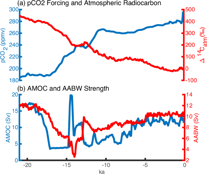
a Surface pCO2 forcing50 (blue line) and the atmosphere Δ14 C51 (red line). b Transports of the Atlantic Meridional Overturning Circulation (AMOC, blue line) and the Antarctic Bottom Water (AABW, red line).
Recently, more sophisticated inverse modeling methods have been proposed as a comprehensive approach to estimate water age from radiocarbon observations16,19,20, along with the joint distribution of surface origin and water age or TTD9,16. DeVries and Primeau21 applied an improved inverse method to infer the ideal age in two deep North Pacific sites, taking into account the mixing from multiple sources by fitting parameterized transit-time distribution-equilibration-time distribution (TTD-ETD). Their estimated age is more accurate than either the B-P age or the projection age, as tested in a model simulation. Nonetheless, all inverse modeling studies so far have been applied using equilibrium or steady-state circulation instead of temporally evolving ocean circulation as during the last deglaciation. In practice, these inverse model studies require substantial coverage of observations and, therefore, may be difficult to apply effectively to the past period when the proxy data are sparse.
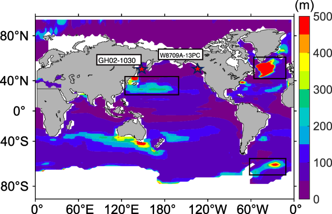
Previous models have shown significant differences between B-P age, B-A age, projection age, and true water ages22,23. This can also be seen in an example in our isotope-enabled ocean-only simulation of the last deglaciation (C-iTraCE). C-iTraCE simulation is a transient ocean model simulation of the past 21,000 years that is forced by the surface climate forcing derived from a transient coupled climate model simulation under realistic climate forcing24 (Fig. 2). The ocean model incorporates multiple geotracers, including radiocarbon25. The deglacial oceanic evolution has been compared with multiple proxy observations with reasonable agreement24,26,27,28,29. We examine the deglacial evolution of the model B-P and B-A ages at two sites in the North Pacific: one shallow site in the intermediate water (at core GH02-103030, 1212 m, Fig. 3a) and one deep site in the deep ocean (at core W8709A-13PC31, 2710 m, Fig. 3b). The B-A and B-P ages in the model show a decreasing trend from the Last Glacial Maximum (LGM) period to the early Holocene (10 ka) at both the shallow and deep sites, such that the model B-P age and B-A age are older at the LGM than 10ka. The older B-A radiocarbon age at LGM than Holocene is a robust feature in observations4,32. The decreasing trends of B-P radiocarbon ages at these two sites are somewhat consistent with observations, as seen in Fig. 3a, b (purple curves), although the absolute age of the deep North Pacific is too old in the model compared with observations, reflecting likely a too sluggish circulation in the abyssal North Pacific in the coarse resolution model. The older LGM B-P ages at the deep site in the deep North Pacific, along with some other sediment records there, have been suggested to reflect a poorer ventilation there at the LGM relative to the present33,34,35,36,37. These deglacial B-P and B-A decreasing trends have led to the controversial speculation that the North Pacific deep water carbon may outgassed to the atmosphere and contributed to the increased atmospheric (C{O}_{2}) during the last deglaciation38,39,40. In our model, the trend of the ideal age (Iage), which is the true water age, is similar to the B-A and B-P ages at the shallow site, but differs dramatically from the B-A and B-P ages at the deep site, where the ideal age increases from 2000 years at 21 ka to 3000 years at ~14–12 ka and then decreases back to 2000 years at 0 ka (Fig. 3b, black). This deglacial evolution of the ideal age is determined mainly by the evolution of the transport of deep circulation, especially the Antarctica Bottom Water (AABW) (Fig. 2b), as studied in a separate work41. Here, instead, we focus on the question: can this true water age be reconstructed, in principle, from marine ({Delta }^{14}C)?
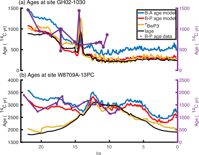
a For site GH02-103030 at 42.23({scriptstyle{circ}atop}{boldsymbol{N}}), 144.21({scriptstyle{circ}atop}{boldsymbol{E}}),1212 m with dominant local water source. b For site W8709A-13PC31 at 42.12({scriptstyle{circ}atop}{boldsymbol{N}}), 125.75({scriptstyle{circ}atop}{boldsymbol{W}}),2710 m with a dominant remote water source. a, b share the same legend, B-A age (blue line), B-P age (red line), radiocarbon age of BwP (yellow line, BwP3), Ideal age (black line), purple dots and lines are sites B-P age. The unit of Iage is model year, while other ages are 14C yr.
The major objective of this paper is to develop a method to estimate the pure water age from radiocarbon in the so-called Benthic minus-weighted Planktic age (BwP radiocarbon age or BwP age). In BwP age, the age of source surface water is estimated from multiple surface planktonic ages weighted by their respective water mass composition contributions to the deep water site, and these water mass compositions are estimated from idealized dye tracers in an ocean circulation model. The issue of projection age is further taken into account using an iteration approach. In essence, this approach is a simplified time-dependent Green’s function approach in the presence of temporally evolving circulation and also accounts for the projection age, where the key element of Green’s function is estimated from an ocean model using water mass composition indicated by dye tracers. Using an ocean model as the testbed, we show that the BwP age reproduces the ideal age by eliminating the differences between B-P, B-A ages and Iage dramatically, due to the consideration of the effects of remote and multiple sources as well as the projection age. Some implications of real-world application of the BwP age are also discussed.
Results
Reconstruction of the ventilation time in the North Pacific with BwP age
To evaluate the reconstruction of BwP age on water age, we will study in detail the two sites in the North Pacific as discussed earlier in Fig. 3: site GH02-1030 and W8709A-13PC. For the shallow site GH02-1030, the water is dominated by the single source of local NP source water for almost the entire 21,000 years (Fig. 4b), leading to the composite endmember ({Delta }^{14}{C}_{S}=mathop{sum }nolimits_{n=1}^{6}{dy}{e}_{n}{Delta }^{14}{C}_{{Pn}}approx {Delta }^{14}{C}_{p,{NP}}) (Fig. 4c). As such, the B-P age of the first 4 iterations all converge to the Iage (Figs. 3a and 4a). This is the special case of dominant local source water, in which the B-P age can be used to reconstruct the water age, as expected. The B-A age is older because of the air-sea exchange and reservoir age, as expected, and therefore will not be our focus hereafter.
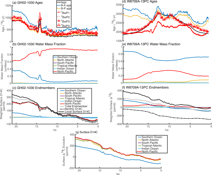
a Ages in site GH02-1030. Ideal age (black), B-A age (blue), B-P age (yellow), and BwP ages of iterations 1–4 (red lines, dots for ({{boldsymbol{tau }}}_{{boldsymbol{BwP}}{bf{1}}}), dashed line for ({{boldsymbol{tau }}}_{{boldsymbol{BwP}}{bf{2}}}), asterisks for ({{boldsymbol{tau }}}_{{boldsymbol{BwP}}{bf{3}}}) and triangles for ({{boldsymbol{tau }}}_{{boldsymbol{BwP}}{bf{4}}})). b Water mass fraction in site GH02-1030. Water mass from the Southern Ocean (dark blue), the North Atlantic (yellow), the South Pacific (purple), the Tropical Atlantic (green), the Indian Ocean (blue), and the North Pacific (red). c Endmember evolution, calculated by multiplying deep convection region surface radiocarbon by its weight (({{{boldsymbol{dye}}}_{{boldsymbol{n}}}{boldsymbol{times }}{boldsymbol{Delta }}}^{{bf{14}}}{{boldsymbol{C}}}_{{boldsymbol{Pn}}})), with the line colors corresponding to those in (b). Additionally, the gray line represents the sum of weighted surface radiocarbon, and the black solid and dashed line represent the benthic and local surface radiocarbon in GH02-1030, respectively. d–f same as a–c, but in site W8709A-13PC. g is deep convection region surface radiocarbon evolution; the legend is the same as (b). The unit of Iage is model year, while other ages are 14C yr.
In contrast, at the deep site W8709A-13PC, the B-P age (and also B-A age) showed two major differences from Iage. First, the B-P age overestimates the Iage dramatically, especially during the early glacial period and towards the PI. Second, the evolution pattern of B-P age is dominated by a declining trend with the LGM older than the PI by ~500 years, while the Iage exhibits a bell-shaped evolution with the LGM slightly younger than PI, and the oldest water achieved ~14–12 ka. These two major differences in the B-P age are reduced dramatically in the BwP age. For this site, the BwP age is much closer to Iage than B-P age (Figs. 3b and 4d). The BwP age converges, after three iterations, as the 4th iteration ({tau }_{{BwP}4}) is almost similar to the 3rd iteration ({tau }_{{BwP}3}). Note that, as the iteration proceeds, the BwP age converges towards an older age. In particular, the old correction from the first guess is the greatest in the period of 14–10 ka, as seen in the difference between ({tau }_{{BwP},n}(n=mathrm{2,3,4})) and ({tau }_{{BwP}1}) in Fig. 4d. This is because the local ({Delta }^{14}C) experiences the most rapid decline before this period (Fig. 4f).
The success of the BwP age in representing the ideal age can be understood through the temporal evolution of the compositional contributions. Throughout the last 21,000 years, the evolution of each water composition (({dy}{e}_{n})) shows that the SO endmember, or the AABW, is the dominant source water, accounting for 60–85% of the site W8709A-13PC deep water (Fig. 4e). This dominant of SO water mass at the present is consistent with other independent estimation using the observation of radiocarbon and other tracers for the present day9. The surface radiocarbons in different dye release regions (({Delta }^{14}{C}_{{Pn}})) largely follows the decreasing atmospheric radiocarbon ({Delta }^{14}{C}_{A}) (Fig. 2a), with particularly the SO ({Delta }^{14}{C}_{P}) depleted by about 200 per mil relative to other sources throughout the deglaciation (Fig. 4g), including the later period towards PD when the lower ({Delta }^{14}{C}_{P}) in SO than other regions is consistent with the surface map of ({Delta }^{14}C) at PD in later Fig. 11. The W8709A-13PC total composite source water ({Delta }^{14}{C}_{s}=mathop{sum }nolimits_{n=1}^{6}{dy}{e}_{n}{Delta }^{14}{C}_{{Pn}}) as derived from the weighted sum of all endmembers (({in; dy}{e}_{n}times {Delta }^{14}{C}_{{Pn}})) shows that the deglacial evolution is dominated by that of the SO endmember (gray vs dark blue, Fig. 4f), consistent with the dominant contribution of SO source water (Fig. 4e). Since the SO surface source ({Delta }^{14}{C}_{{Pn}}) is significantly lower than other sources (by about 200 per mil, blue vs others, Fig. 4g), the total composite ({Delta }^{14}{C}_{S}) is much lower than local ({Delta }^{14}C) (by ~200 per mil, gray vs black line in Fig. 4f). This leads to a much younger BwP age than B-P age throughout most of the last 21,000 years, in the first guess ({tau }_{{BwP}1}) (Fig. 4d). Thus, the BwP age enables the realization of the ideal age estimation by including the contribution of remote sources, particularly from SO. Towards the 14–10 ka, about a third of the SO water is replaced by the local NP source water (Fig. 4e), as such the ({Delta }^{14}{C}_{S}) approaches NP ({Delta }^{14}{C}_{P}) (Fig. 4f) and BwP age is close to the B-P age, while B-P age is substantially older than BwP at the LGM. Later towards Holocene, the opposite occurs, because the contribution of SO water increases again (Fig. 4e, f), such that the BwP age becomes substantially younger than the B-P age, with the former close to Iage. Overall, during the entire deglaciation, the dominant source of SO water leads to ({Delta }^{14}{C}_{S}approx {Delta }^{14}{C}_{P,{SO}}), and, therefore this site is an extreme case dominated by a single remote source, such that the B-P age is biased too old.
The radiocarbon evolution of the deep site W8709A-13PC seems representative of other cores in the deep North Pacific, because all these sites share the same dominant SO remote source. We selected several other sites in the North Pacific, and the mean B-P age of these sites shows a nearly flat to slightly declining trend from the LGM to a somewhat younger PD (markers and the gray line in Fig. 5). The model mean B-P age averaged over these sites shows a somewhat similar evolution to the proxy, with the LGM slightly older than the PD, although the model overestimates the older ages in between (blue broken line in Fig. 5). This model mean B-P age differs from the Iage significantly, while the Iage, however, is reproduced almost perfectly by the mean BwP age, as discussed for the site of W8709A-13PC (Figs. 3b and 9d). This suggests that the deep North Pacific may not be much older at the LGM than at the PD in terms of water age as suggested by some previous studies33,34,35,36,37. Stott40 has recently suggested that the older radiocarbon ages in the deep core data in North Pacific can be affected by other processes, such as the low sediment rate and bioturbation. Other processes such as sea floor hydrothermal activities and methane seeps may also affect the ({scriptstyle{14}atop}C/{scriptstyle{12}atop}C) ratios of fossil biogenic carbonates42,43. Our study offers another possibility of an inaccurate B-P age estimation.
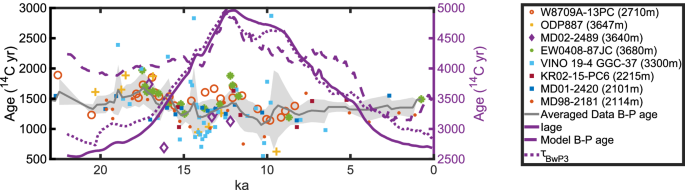
Dots are B-P ages in site data. Red circles for W8709A-13PC31 (42.12°N, 125.75°E, 2710 m), yellow cross markers for ODP88752 (54.62°N, 148.75°E, 3647 m), purple diamonds for MD02-248953 (54.39°N, 148.92°E, 3640 m), green asterisks for EW0408-87JC54 (58.77°N, 144.5°E, 3680 m), blue circles for VINO 19-4 GGC-3732 (50.40°N, 167.70°E, 3300 m), maroon circles for KR02-15-PC655 (40.40°N, 143.50°E, 2215 m), dark blue circles for MD01-242056 (36.07 °N, 141.82 °E, 2101 m), red dots for MD98-218157 (6.30°N 125.80°E, 2114 m). Gray solid line and shading are the mean age of sites above with one standard error, the purple solid line, purple dashed line and purple dotted dashed line are mean model Iage, B-P age and ({{boldsymbol{tau }}}_{{boldsymbol{BwP}}{bf{3}}}) at same sites locations, respectively. The unit of Iage is the year in the model, while other ages are 14C yr.
Reconstruction of the ventilation time in the North Atlantic with BwP age
We now evaluate the BwP age in the North Atlantic. We first selected several sites in the North Atlantic at depths greater than 2000 meters and compared the observed B-P ages with model results (Fig. 6). The observed B-P ages show a slight increasing trend from the LGM to the early deglaciation period, followed by a sharp decrease ~14 ka, a slight increase until 13 ka, and then a gradual decline toward the present day (gray line in Fig. 6), as in previous studies5,32. This slow evolution trend is largely reproduced in the model B-P age (broken tangerine red line in Fig. 6), although the model B-P age is overall older than in observations, similar to the deep North Pacific as discussed above. Note that in Skinner (2023)5, the basin age was determined using Bayesian interpolation, whereas in this study, we calculated the basin age simply using the raw data average. Despite the methodological differences, our raw data and Skinner (2023)5 reveal consistent age trends in the deep Atlantic. For our purpose to test BwP method, here, our model BwP ages successfully reproduce the evolution of the ideal age (dotted and solid tangerine red lines in Fig. 6), as in the North Pacific discussed above.
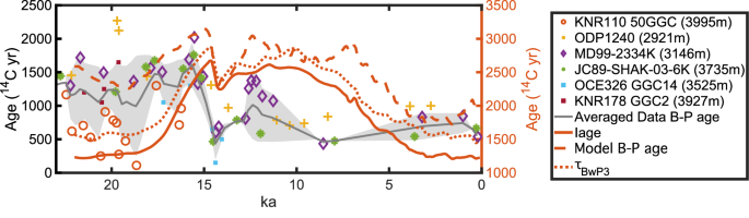
Dots are B-P ages in site data. Red circles for KNR110 50GGC2 (4.87°N, 43.22°W, 3995 m), yellow cross markers for ODP124058 (0.02°N, 86.46°W, 2921 m), purple diamonds for MD99-2334K7 (37.80°N, 10.17°W, 3146 m), green asterisks for JC89-SHAK-03-6K59 (37.71°N, 10.49°W, 3735 m), blue circles for OCE326 GGC1460,61 (43.07°N, 55.83°W, 3525 m), maroon circles for KNR178 GGC262 (36.12°N, 72.29°W, 3927 m). Gray solid line and shading are the mean age of sites above with one standard error, the tangerine red solid line, tangerine red broken line and dotted dashed line are mean model Iage, B-P age and ({{boldsymbol{tau }}}_{{boldsymbol{BwP}}{bf{3}}}) at same sites locations, respectively. The unit of Iage is model year, while other ages are 14 C yr.
The data-model comparison in the deep Atlantic shows better agreement than in the deep Pacific, as the model accurately captures the B-P age trend in the Atlantic. In the deep North Pacific, the model significantly overestimates the B-P age ~14 ka. This discrepancy may be attributed to the model’s underestimation of AABW strength during HS1 (Fig. 2b). Since AABW is the dominant water mass in the deep North Pacific, a weaker simulated AABW would result in reduced radiocarbon ventilation in this region, leading to an overestimation of the ideal age during the subsequent period. The simulated weaker AABW at HS1 may be caused by inaccurate deep water formation region in Southern Ocean (Fig. 14). Overall, despite some overestimation of the deep Pacific ages during the intermediate period ~14 ka, our model corresponds reasonably well with the slow evolution trend of the B-P ages in observations, especially in Atlantic. It is nevertheless important to emphasize that our primary objective is to develop a radiocarbon age calculation method capable of accurately reproducing the ideal age. This objective is tested valid in the ocean model, and this validation does not require the model to perfectly match the real world.
Discussion
The success of BwP age in estimating the true water age (Iage) is not limited to the few sites in the North Pacific and North Atlantic, but globally in our model. First, BwP age dramatically reduces the difference between B-P, B-A ages and Iage. Second, instead of exhibiting a generally decreasing trend as in B-P and B-A ages, the BwP ages peak in the middle of ~14 ka, closely resembling the Iage.
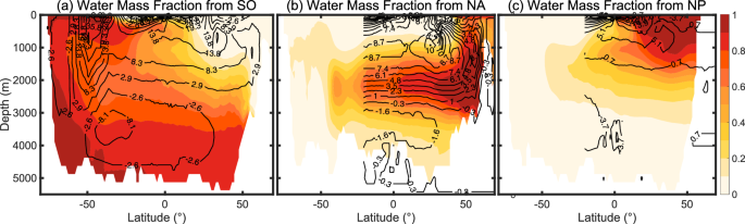
Fig. 7 shows the comparison of BwP age, B-P age, and B-A age with the Iage averaged zonally for both Pacific and Atlantic at the LGM, 14 ka, and PI. In both Pacific and Atlantic, a visual inspection shows that both B-A and B-P ages overestimate the Iage substantially at all three times. These older differences are reduced significantly in the BwP age (({tau }_{{BwP}3})) (Fig. 7). For example, during the LGM in the Pacific, the age of the oldest water in the northern deep ocean is ~2000 years in Iage, 2000 years in BwP age, but over 2800 years in B-P and B-A ages. The systematically older B-A than B-P age is caused by the marine reservoir age.
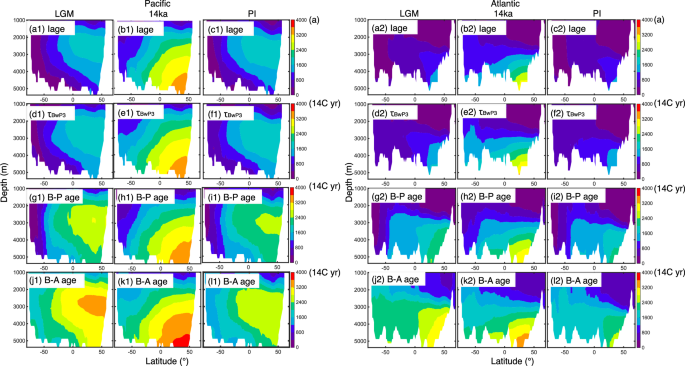
a1, b2, c1 for Iage in Pacific at the LGM, 14 ka and PI, respectively, d1, e1, f1 same as a1, b1, c1 but for BwP3 age. g1, h1, i1 same as (a1), (b1), (c1) but for B-P age. (j1), (k1), and (l1) same as (a1), (b1), and (c1) but for B-A age. The right panels are the same as the left panels but for Atlantic.
The W8709A-13PC site and GH02-1030 site in the deep North Pacific discussed above represent two extreme cases, with the former dominated by the remote source and the latter dominated by the local source. Most other regions are a mixture of remote and local sources with the differences between the B-P age and Iage varying from site to site. This spatial variation of the B-P age difference from Iage can be seen in zonal mean root mean square error (RMSE) in the Atlantic and Pacific basins in Fig. 8a, c. Overall, below 2000 m, the North Pacific exhibits a large difference because of the dominance of the remote SO source (Fig. 8c, d), while the mid-depth North Atlantic exhibits a small error because of the dominance of the local source (Fig. 8a, b). The SO has minimum difference because of the dominance of its local source water. In other regions, the water mass consists of a mixture of both local and remote sources, and the differences are intermediate.
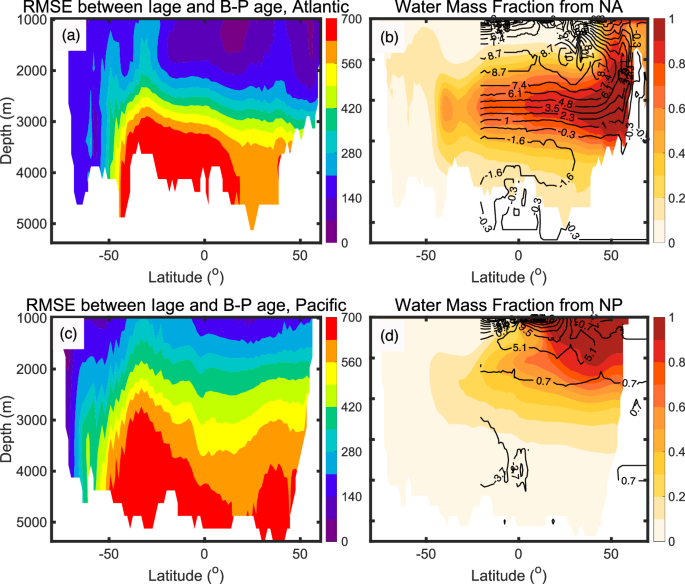
a, c depict the RMSE values of B-P age from the Iage, across the Pacific and Atlantic basins. b, d illustrate the water mass fraction of NA and NP in the Atlantic and Pacific oceans during PI. The contours in (b) and (d) are the streamfunctions of the overturning in the Atlantic and Pacific, respectively.
Fig. 9 shows the scatter diagram of the RMSE and correlation of various radiocarbon ages and Iage for waters below 1000 m in different parts of the world ocean, each dot being a grid point. The RMSE of deep water below 2000 m is over 700 years in B-A age, over 500 years in B-P age, but <250 years in BwP age (Fig. 9a, c). The errors systematically greater than a lower threshold of 500 years in the case of B-A age reflect the existence of surface reservoir age (Fig. 9c). Furthermore, the temporal correlation with Iage is almost all positive for BwP age, but nearly half negative for B-P and B-A ages (Fig. 9b, d). The dramatic difference in the temporal correlation suggests that the differences between B-P, B-A ages and Iage lead to dramatically different evolution behaviors from the truth instead of a constant offset of older age. This error in temporal evolution behavior is largely corrected in BwP age.
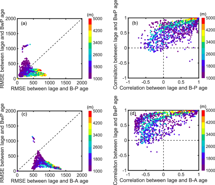
a The root mean square error (RMSE) of the B-P age from Iage (averaged over the 21,000 years) versus the BwP age (({{boldsymbol{tau }}}_{{boldsymbol{BwP}},,{bf{3}}})) from Iage at each grid point below 1000 m in the global ocean. b same as (a) but for the temporal correlation coefficients between the B-P age and Iage, versus those between BwP and Iage. c, d the same as (a) and (b), respectively, but with the B-A age replacing B-P age. Color represents the depth of each grid point.
One distinct feature of our BwP age is that it can be used conveniently for water age estimation under temporally changing ocean circulation and, therefore, can be used to assess the impact of varying circulation on age estimation. In comparison, inverse methods so far are performed on steady circulations. The effect of changing circulation is reflected in the change of dye distribution in the simulation naturally. Thus, the effect of the changing circulation can be estimated by comparing the BwP age of temporally varying dye with the nominal BwP age that is estimated using the dye concentration at a fixed time. Fig. 10 shows the comparison of the BwP age in comparison with the nominal BwP age using the dye concentration at the LGM and PI (red and yellow lines in Fig. 10). The nominal BwP age of LGM (PI) dye can be thought as the water age that is formed by the fixed circulation at the LGM (PI), and therefore its difference from the BwP age of varying dye is caused by the changing circulation. At first sight, the two nominal BwP ages with fixed dye weights appear to be able to reproduce the qualitative features of the Iage evolution, which are characterized by a bell-shaped pattern with an age peak at about 12 ka. Quantitatively, nevertheless, these nominal BwP ages differ from the BwP age and Iage. For example, in the deep North Pacific site, using the PI dye, the nominal BwP age at the LGM is about 20% younger than the ideal age, while the BwP age is less than 10% younger than the ideal age (Fig. 10f). Overall, the biases of the two nominal BwP ages are greater than that of the BwP age using the temporally evolving dye weight.
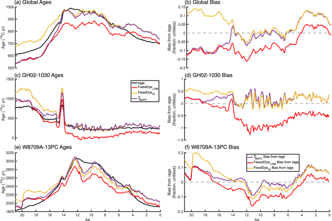
a shows the global average of BwP age with varying dye (purple), and the nominal BwP ages using dye at the LGM (red) and PI (yellow) dye, in comparison with the ideal age (black). b shows the corresponding difference between the three BwP ages and the ideal age as a fraction of the absolute ideal age (BwP age- Iage)/Iage. c, d are the same as (a) and (b), respectively, but for Site GH02-1030; e, f are the same as (a, b), respectively, but for Site W8709A-13PC.
The RMSE profiles of BwP ages also show a better consistency between BwP age and the Iage with varying dye than with fixed dye (Fig. 11). Below 1000 m, the mean RMSE values between Iage and BwP with varying dye, BwP with fixed LGM dye, BwP with fixed PI dye are 71.7, 184.5, and 237.0, respectively.
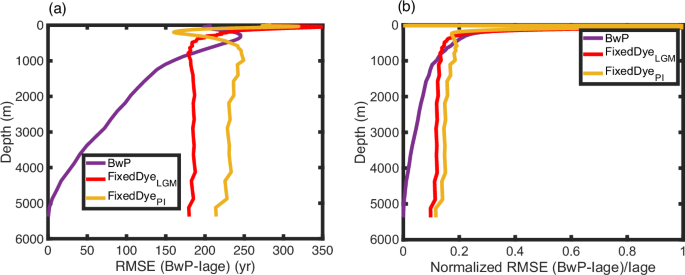
a shows the RMSE value (left(root{2}of{frac{{sum }_{{boldsymbol{1}}}^{{boldsymbol{n}}}{left({boldsymbol{BwP}},{boldsymbol{n}}-{boldsymbol{Iage}},{boldsymbol{n}}right)}^{{boldsymbol{2}}}}{{boldsymbol{n}}}}right)) between Iage and BwP age with varying dye (purple), nominal BwP age using dye at the LGM (red), and nominal BwP age using dye at the PI (yellow). b is same as (a), but for RMSE value as a fraction of the absolute Iage.
Overall, the BwP age method is developed to reconstruct the pure water age from radiocarbon observations, with the aid of a model simulation of the water composition. The method is tested in an ocean model successfully. The BwP age reproduced the pure water age globally. It effectively removes those age differences in the B-P and B-A ages, especially at depths >1000 m, where the RMSE of BwP age is much lower. The BwP age also demonstrates a temporal correlation with the true water age (Iage) that is consistently positive, in contrast to the negative correlations often observed in B-P and B-A ages, indicating that BwP age better captures the actual evolution of water masses. Additionally, BwP age is capable of adapting to varying ocean circulation patterns, offering a dynamic assessment of water age under changing conditions. This flexibility further emphasizes the importance of using transient changing dye, highlighting the limitations of the TTD method in paleo-climate studies. The comparison of BwP age with nominal BwP ages, which use fixed dye concentrations at different time points (LGM and PI), further emphasizes the superior performance of BwP age in reflecting the true age of water masses. In principle, BwP age offers a more accurate, adaptable, and dynamic approach to estimating water age across different ocean regions and time periods.
An application of our BwP age to the observations in the deep North Pacific suggests that the true water age at the LGM may not be much older than the present, as was implied from the B-P age. This real-world application, however, should be taken with caution because of one major limitation of the BwP age to the real world. In addition to observations of marine radiocarbon measurements, our BwP method also depends on the water composition that has to be derived from a model simulation. Therefore, the estimation of real-world BwP age, and pure water age, will depend on the realism of this model simulation. Here, our model simulation shows some consistency with observations during the deglaciation in terms of the B-P ages, as well as some other marine proxies26,27. Therefore, the model water composition evolution may be of some relevance to the real world. Thus, we feel that our results on the comparable deep North Pacific pure water ages between the LGM and the present may still be reasonable. Future studies with improved model simulation are needed to further test this result for the real world.
Methods
The isotope-enabled ocean model
In this study, we use the ocean model of Parallel Ocean Program version 2 (POP2)44, which is the ocean component of the Community Earth System Model (CESM). The resolution is 3° horizontal with 60 vertical levels. Several isotope-based tracers have been incorporated into POP2, including radiocarbon25, creating a new version called iPOP2. The simulated radiocarbon under modern forcing25 compares reasonably well with the Global Ocean Data Analysis Project (GLODAP)45. At the surface, the ({Delta }^{14}C) reached its minimum in the Southern Ocean, due to the sea ice insolation effect and upwelling of old water, consistent with the present GLODAP observations (Fig. 12a). Vertically, the ({Delta }^{14}C) pattern is also reasonably consistent with the present GLODAP observation in the deep ocean. For example, in the Pacific, the minimum ({Delta }^{14}C) is located in the mid-depth of the North Pacific (Fig. 12b), while in the Atlantic, ({Delta }^{14}C) is enriched towards the north at mid-depth (Fig. 12c).
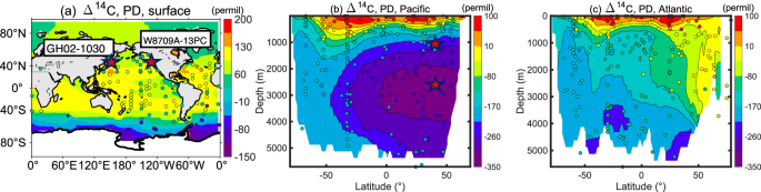
Simulated present day (PD) radiocarbon distribution (a) on the sea surface, b, c zonally averaged in the Pacific and Atlantic basin, respectively. The overlaid dots in the diagram correspond to observational records sourced from The Global Ocean Data Analysis Project (GLODAP)45. The red stars are sites GH02-1020 (upper) and W8709A-13PC (lower). The PD simulation is from Jahn et al.25.
The iPOP2 has been used to simulate the transient evolution of the ocean from 20 ka to the 0 ka (called C-iTraCE26). In C-iTraCE, iPOP2 was forced by monthly surface forcing that is derived from a coupled transient simulation (TRACE21)46. The C-iTraCE has been compared directly against multiple marine proxies with good agreement24,29, suggesting that the deglacial evolution of ocean circulation and water masses was reasonably simulated. The initial condition for carbon isotopes was set as follows: (p{{CO}}_{2}) as 188 ppmv, and ({Delta }^{14}C{O}_{2}) as 398‰ and 394‰ in the Northern Hemisphere and Southern Hemisphere, respectively28. The ({pC}{O}_{2}) and atmospheric ({Delta }^{14}C) evolution in C-iTraCE is shown in Fig. 2a.
The model also simulated the ideal age (Fig. 3). The ideal age was set to 0 at the ocean surface and increased at the rate of 1 yr/yr in the ocean interior. In an ocean model, the weights of different source waters, or the water mass composition, can be simulated using idealized dye tracers27. In C-iTraCE, six dye tracers were simulated, which were released from the surface North Atlantic (NA), tropical Atlantic (TA), Southern Ocean (SO), North Pacific (NP), South Pacific (SP) and Indian Ocean (IO), respectively (Fig. 13a–f). For each dye, the tracer value was prescribed as 1 (0) in the sea surface inside (outside) the source region at each time step.
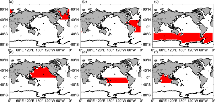
Dye tracers from (a) North Atlantic (north of 40°N), b subtropical Atlantic (34°S–40°N), c Southern Ocean (south of 34°S), d North Pacific (north of 0 in Pacific), e South Pacific (34°S-0 in Pacific) and f Indian Ocean (34°S-0 in Indian Ocean).
Spin up details
The physical circulation, ideal age, and radiocarbon were initialized from the LGM spin-up in Zhang et al.47, which has been integrated for more than 10,000 years under LGM forcings. Then, the model is further integrated for an additional 4788 years under repeated forcings of 22 ka–20 ka. The dye tracers were initialized from dye distributions at modern conditions and spun up under LGM forcings for more than 3000 years until the dye tracers in the abyssal ocean reached quasi-equilibrium.
The calculation of BwP radiocarbon age
To motivate our new scheme, we start with some idealized scenarios. Given a measured radiocarbon concentration of benthic ({{bf{14}}atop}{boldsymbol{C}}_{{boldsymbol{B}}}) in the deep water, if it is derived completely from a single source of surface concentration ({14atop}C_{{boldsymbol{S}}}), the radiocarbon age can be calculated as:
where λ = 1/8267 year−1 is the decay constant3. If the source is a single one without mixing, then the radiocarbon age, or radiocarbon ventilation time, will be the same as the true ideal age or ventilation time10,48. If the source happens locally right at the benthic site, the ({{14 atop}C}_{S}) can be substituted by the local surface phytoplankton ({{14 atop}C}_{p}) (({{14 atop}C}_{p1}) in Fig. 1) and this ventilation time (1) is just the B-P age:
In general, however, the source water may originate remotely, often far away from the benthic site, with a radiocarbon concentration ({{14 atop}C}_{p2}) different from the local ({{14 atop}C}_{p1}) (as shown schematically in Fig. 1), leading to a difference between the B-P age and the ideal age. For example, in the deep North Pacific, the source water originates mostly from the Southern Ocean, where the ({{14 atop}C}_{p2}) is much more depleted than the local ({{14 atop}C}_{p1}) in the North Pacific (Fig. 11a). The B-P age Eq. (2) using the local ({{14 atop}C}_{p1}) will then lead to a much shorter radiocarbon ventilation time than the true ventilation time, that is:
More generally, ocean water mass at a deep site is often contributed by multiple sources, as shown schematically in Fig. 1, such that the radiocarbon concentration is a mass-weighted average of the surface radiocarbon from all the sources:
where ({W}_{n}) is the water mass fraction from source “n”. The radiocarbon age calculated using Eq. (3) will be biased towards those of the shorter sources10.
The water masses originate from the North Atlantic, Southern Ocean, and North Pacific and correspond approximately to the three major deep water masses of the AABW, North Atlantic Deep Water (NADW), and North Pacific Intermediate Water (NPIW), respectively. As such, at any location in the deep ocean, the value of each dye represents the weight, or water mass fraction, of this endmember ({w}_{n}={dy}{e}_{n}) and the total sum of all dyes is always 1. For example, Fig. 14a–c shows the global zonal mean distributions of the SO dye, NA dye, and NP dye at the PI, which represent the weights of AABW, NADW, and NPIW, respectively. SO dye is >0.6 below 3000-m over most of the global ocean, suggesting the dominant contribution of the AABW over 60% to the global abyss (Fig. 14a). The NA dye forms a maximum tongue of up to 0.3–0.4 in between 1500 m and 3000 m (Fig. 14b), confined mainly in the Atlantic basin, suggesting the NADW as the other major deepwater mass. The NP dye is confined in the northern upper ocean above 2000m (in the North Pacific, Fig. 14c), reflecting the contribution of the NPIW dominant only in the North Pacific upper ocean. The inferred deepwater composition is qualitatively consistent with present observations8. Thus, ({w}_{n}={dy}{e}_{n}(vec{x},t)), where (vec{x}=(x,y,z)) is the space vector. The detailed change of the deepwater masses and the mechanism have been discussed separately28,41 and will not be discussed here.
a–c for dye distribution from Southern Ocean, North Atlantic, and North Pacific, respectively. a–c are global, Atlantic basin, and Pacific basin zonal mean respectively. The stars in (c) are sites GH02-1020 (upper) and W8709A-13PC (lower).
These dye tracers provide a comprehensive estimation of the weights of different source waters. This allows us to design the BwP age for estimating the water age. The BwP age reduces two major differences of the B-P age from the ideal age in two steps: step 1 corrects the age difference associated with remote and multiple sources, while step 2 corrects the age difference caused by the temporal evolution of atmospheric radiocarbon, or the projection age.
Step 1: Correction for multiple sources: This step is calculated as in the B-P age, except that the source water radiocarbon is estimated using the weighted sum in Eq. (3), or in terms of ({Delta }^{14}C) (in per mil)49
as
with the ({Delta }^{14}{C}_{{Pn}}left(vec{x},tright)) corresponding to the average of ({Delta }^{14}C) over the surface of the source region where dye was released. PIPN means preindustrial prenuclear atmosphere. Here, we have assumed, approximately, the change of ({Delta }^{14}C) is caused mainly by the decay of ({14atop}C), with the ({12 atop}C) taken as a constant. The 1st guess of BwP age is then estimated from eqns. Eq. (1) and Eq. (4a) in ({Delta }^{14}C) as
This step of BwP takes into account the multiple sources, remote and local, and therefore is expected to reduce the source difference of the B-P age. For example, in the abyssal North Pacific, the dominant source water ({Delta }^{14}{C}_{{Pn}}left(vec{x},tright)) from PI to LGM is the remote AABW, instead of the local NPIW (Fig. 14). Therefore, the BwP age should reduce the difference of the B-P age associated with the remote source water.
It is tempting to estimate the source ({Delta }^{14}{C}_{{Pn}}left(vec{x},tright)) simply as the surface ({Delta }^{14}{C}_{P}left(vec{x},tright)) value spatially averaged over the entire region of each dye as prescribed in Fig. 13. This estimation, however, differs from Iage for deep water sources, such as AABW, NADW, and NPIW in our dye tracers. These deep water masses are formed in isolate regions of deep convection, over which the ({Delta }^{14}{C}_{P}) could differ substantially from the average over the entire region of surface dye prescription (compare Fig. 12 with Fig. 13). To increase the accuracy of the estimation, we estimate the ({Delta }^{14}{C}_{{Pn}}) for the deep water endmembers by limiting the average over the subregions of deep convection, as outlined in square boxes in Fig. 15. In future studies, this uncertainty can be reduced by rerunning the simulation with increased number of dye tracers with some tracers directly sourced from the deep convection regions.
The black boxes are deep convection over which the mean radiocarbon is used for the calculation of the weights for the BwP age from the North Pacific, North Atlantic, and Southern Ocean. The red stars are sites GH02-1020 and W8709A-13PC.
Step 2: Correction for projection age: aside from the problem of sources, the B-P age is also different from Iage by the temporally varying atmosphere ({Delta }^{14}{C}_{A}) in the so-called projection age13. In our BwP method, the projection age is estimated using an iteration approach as follows. With the first guess ({tau }_{{BwP}1}) in Eq. (4a, b), we will re-estimate the BwP age but using the surface ({Delta }^{14}{C}_{{Pn}}) of a lead time ({tau }_{{BwP}1}) earlier. That is, we can use Eq. (4a, b) again, but with a lead of ({tau }_{{BwP}1}) as
Here, as an approximation, the water mass composition value is the average between the lead time and current time. In general, for the ith iteration, we have
In principle, the iteration proceeds until it converges. In practice, we find that the convergence is fast and 3 iterations are sufficiently accurate. Thus, unless otherwise specified, we take ({tau }_{{BwP}3}) as BwP age.

Responses