Increased longitudinal separation of equatorial rainfall responses to Eastern Pacific and Central Pacific El Niño under global warming

Introduction

The El Niño-Southern Oscillation (ENSO), the strongest air-sea interaction mode of the climate system^1,2,3,4, leads to year-to-year climate anomalies all around the world. It affects many aspects of human activities and natural systems, such as water resources, fishing, agriculture, finance, coastal erosion, land and marine ecosystems^{3,5,6,7,8,9,10}. These global climate impacts of ENSO are forced mainly through anomalous tropical convective heating and its excited atmospheric teleconnections^{3,5,6,11,12,13,14,15,16}.

ENSO-related teleconnections and global climate variations are complicated by a diversity of ENSO spatial patterns^{14,17,18,19,20,21,22,23,24,25}. Two typical types of El Niño, eastern Pacific (EP) and central Pacific (CP) El Niño, named after the central positions of their sea surface temperature (SST) anomalies, drive tropical precipitation and its associated convective heating anomalies with remarkable longitudinal shifts. Correspondingly, the anomalous Walker Circulation and the Pacific-North American (PNA) teleconnection pattern associated with CP El Niño are shifted westward relative to those associated with EP El Niño^{14,17,18,19,24,26,27,28}. As a result, different climate impacts of two types of El Niño are also observed in Asia and Australian monsoon domain^19,29, North America^26,27, South America^12,15 and polar region^25,30.

ENSO is projected to undergo significant changes under global warming according to state-of-the-art coupled climate system models^{31,32,33,34,35,36,37,38,39,40,41,42,43,44}. Most climate models project an El Niño-like warming pattern in the background mean state of tropical Pacific, while observational records show a La Niña-like mean state change over the past century. Uncertainty in the change in the background mean state introduces additional complexity and uncertainty in ENSO projections^41,45,46. Compared with large uncertainties in the variation of ENSO intensity influenced by internal variability and external forcing^32,39,47,48, ENSO-driven precipitation anomalies over the equatorial Pacific are projected to shift eastward under global warming with high inter-model consensus^{49,50,51,52,53,54,55,56}. This is associated with El Niño-like warming of the mean-state SST^{35,49,50,51,52}, changes in ENSO-driven vertical motion anomalies^{35,53,54,55,56}, and meridional narrowing of ENSO SST anomalies⁵⁶. The robust change in tropical convective heating anomalies further causes the anomalous Walker Circulation and PNA teleconnection pattern to shift eastward^{12,13,41,56,57,58,59,60,61,62}. However, whether changes in the EP and CP El Niño-driven precipitation anomalies differ under global warming remains unexplored. In this study, we show evidence that the eastward shift of ENSO precipitation anomalies is present mainly in EP El Niño and is not visible in CP El Niño, which leads to greater differences in their global climate impacts under global warming.

Results

Increased longitudinal separation in precipitation anomalies

The maximum of positive precipitation anomalies over the equatorial Pacific, driven by EP El Niño, is located to the east of that driven by CP El Niño by about 16 longitudinal degrees in the multi-model ensemble mean of historical simulations from the sixth phase of the Coupled Model Intercomparison Project (CMIP6) (Fig. 1a, d, Methods), consistent with that in observations²⁴. Under the shared socioeconomic pathway 5-8.5 scenario (hereafter SSP585, used here to identify the signal clearly), the distance in longitudinal positions is projected to increase by about 15 degrees longitudes, widening to 27 degrees (Fig. 1b, e, Supplementary Fig. 1 and Supplementary Table 2). The increased difference in the longitudinal positions of the precipitation maxima is mainly due to the significant eastward shift of EP El Niño-driven precipitation anomalies, as confirmed by a two-tailed Student’s t-test at the 5% significance level. While the CP El Niño-driven precipitation maximum undergoes virtually no change, exhibiting only an insignificant slight westward shift. The increased longitudinal separation in the precipitation anomalies is reproduced by 13 of 15 models, with only two models (CanESM5 and GFDL-CM4) showing an opposite, decreased separation feature (Supplementary Fig. 1a). The increased separation in the longitudinal positions is robust and not dependent on the definition of the center of precipitation anomalies (Fig. 1g, h and Supplementary Fig. 1). For example, the distance between the centroids of the precipitation anomalies (defined as the longitude-weighted integral of positive precipitation anomalies) associated with CP and EP El Niño is projected to increase from 28 degrees to 41 degrees in the ensemble-mean simulations (Supplementary Fig. 1b).

Increased longitudinal separation of equatorial rainfall responses to Eastern Pacific and Central Pacific El Niño under global warming — **Fig. 1: Simulated changes in SST and precipitation anomalies during the EP and CP El Niño mature winter under global warming.**

In contrast to the increased differences in the longitudinal positions of the precipitation anomalies between EP and CP El Niño events, the central positions of SST anomalies are projected to remain almost unchanged (Fig. 1a, b, d, e and Supplementary Fig. 2). For both types of El Niño, positive precipitation anomalies are located west of the main body of warm SST anomalies in present-day and future conditions. This is due to the nonlinear responses of tropical convection to underlying SST^23,63,64,65 and the westward shift of SST-gradient-driven boundary-layer convergence anomalies relative to SST anomalies themselves²⁴. In contrast, under global warming, the changes in positive precipitation anomalies for EP and CP El Niño are projected to appear over the equatorial eastern and central Pacific, close to where the variations of El Niño-related SST anomalies ((Delta SST^{prime})) occur (Fig. 1c, f).

Mechanisms for variations in precipitation anomalies

To understand the change in ENSO-driven precipitation anomalies, we performed a moisture budget analysis (Methods). This reveals that the change in precipitation anomalies is dominated by the variations in anomalous convergence of mean-state moisture ((Delta langle -bar{q}{nabla }_{h}cdot overrightarrow{u}^{prime} rangle), Supplementary Fig. 3a, d), while variations in evaporation and moisture advection are negligible (figure not shown). Further, the variation of anomalous convergence of mean-state moisture is primarily caused by the variation of anomalous mass convergence ((-bar{q}Delta langle {nabla }_{h}cdot overrightarrow{u}^{prime} rangle)) for both EP and CP El Niño (Supplementary Fig. 3b, e). As a comparison, the contribution of the increased mean moisture ((langle -Delta bar{q}{nabla }_{h}cdot overrightarrow{u}^{prime} rangle)) is mainly located in the equatorial western-central Pacific for both types of El Niño, outside the main body of the changes in precipitation anomalies (Supplementary Fig. 3c, f). Therefore, the focus is narrowed to physical processes responsible for variations in El Niño-related boundary-layer convergence anomalies under global warming.

The boundary-layer convergence anomalies are connected to El Niño-related SST anomalies through the Lindzen-Nigam mechanism^66,67,68. In the tropics, SST anomalies constrain temperature anomalies in the cumulus boundary layer through cumulus convection and turbulence, which cause boundary-layer pressure gradients and frictional boundary-layer convergence to vary with the underlying SST gradient, rather than the absolute value of SST. It is shown that the zonal distribution of the change in precipitation anomalies ((Delta Pr^{prime})) over the equatorial Pacific closely resembles variation in the second-order meridional derivative of SST anomalies ((-frac{{partial }^{2}}{partial {y}^{2}}(Delta SST^{prime} ))) for both EP and CP El Niño (Fig. 2a, b) in the ensemble mean. The resemblance is more pronounced than with (Delta SST^{prime}) itself, particularly for the EP El Niño (Fig. 1c and Fig. 2a), suggesting the significant influence of the meridional structure of SST anomalies on the overlaying precipitation anomalies through the Lindzen-Nigam mechanism.

**Fig. 2: Simulated changes in El Niño-driven precipitation anomalies under global warming and relationships with changes in the meridional distributions of underlying SST anomalies.**

The crucial role of the longitudinal position of (-frac{{partial }^{2}}{partial {y}^{2}}(Delta SST^{prime} )) in determining the longitudinal position of the change in precipitation anomalies is confirmed in individual models as well as in the ensemble mean (Fig. 2c, d). For EP and CP El Niño, (Delta Pr^{prime}) over the equatorial eastern and central Pacific simulated by individual models is significantly correlated with (-frac{{partial }^{2}}{partial {y}^{2}}(Delta SST^{prime} )) in situ, with their correlation coefficient reaching 0.81 and 0.62 respectively (Fig. 2c, d). Most models fall into the first quadrant of the scatter plots for both EP and CP El Niño, that is, positive (-frac{{partial }^{2}}{partial {y}^{2}}(Delta SST^{prime} )) corresponds to positive (Delta Pr^{prime}), with only 2 exceptions for both types of El Niño, respectively. As a comparison, the correspondences between the (Delta Pr^{prime}) and (Delta SST^{prime}) have larger uncertainties within the model ensemble. For EP El Niño, positive (Delta Pr^{prime}) corresponds to underlying negative (Delta SST^{prime}) in five models (second quadrant, Supplementary Fig. 4a). For CP El Niño, the correlation between (Delta Pr^{prime}) and (Delta SST^{prime}) is only 0.38, which does not reach the 5% significance level based on a bootstrap test (Supplementary Fig. 4b).

The difference in the zonal distribution of (-frac{{partial }^{2}}{partial {y}^{2}}(Delta SST^{prime} )) between EP El Niño and CP El Niño causes their different variations in longitudinal positions of the precipitation centers under global warming. As seen from Fig. 1c, an opposite sign of (Delta SST^{prime}) is evident around the date line, where just the location of EP El Niño precipitation center in the historical runs. Thus, the second-order meridional derivative of SST anomalies must also have such a zonal contrast (Fig. 2a). This leads to a significant eastward shift of the center of the boundary layer convergence and thus the precipitation center. In contrast, for CP El Niño, the zonal variations of SST anomalies and the second-order meridional derivative of SST anomalies around the precipitation center (160°E) are much weaker and without a sign change (Figs. 1c and 2b). Consequently, insignificant zonal shifts occur in the anomalous boundary layer convergence and precipitation centers during CP El Niño under global warming.

The positive (-frac{{partial }^{2}}{partial {y}^{2}}(Delta SST^{prime} )) is caused by the change in the meridional structure of El Niño SST anomalies under global warming. The zonally averaged EP and CP El Niño-related SST anomalies over the equatorial eastern and central Pacific respectively show a hill-like structure with its peak on the equator in the historical runs (Fig. 3a). In the SSP585 simulations, the hill-like structure becomes much steeper for both EP and CP El Niño, corresponding to positive (-frac{{partial }^{2}}{partial {y}^{2}}(Delta SST^{prime} )) (Fig. 3b).

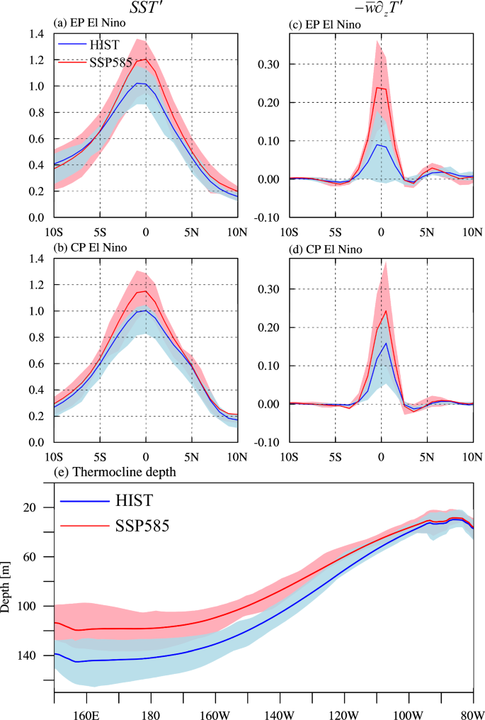
Fig. 3: Meridional distributions of EP and CP El Niño SST anomalies during the El Niño mature winter and associated thermocline feedback during the El Niño developing phase simulated by the historical and SSP585 runs.

To further investigate what causes the equatorial enhancement of El Niño-related SST anomalies under global warming, we diagnose the mixed layer heat budget over the equatorial central and eastern Pacific for the developing phase of CP El Niño and EP El Niño events from May to August, respectively (Methods). From the longitudinal averaging perspective, the change in anomalous SST tendencies in the SSP585 experiments at the equator is larger than those on either side for both CP and EP El Niño (Supplementary Fig. 5c, f and Supplementary Fig. 6a), and this is responsible for the steepening of the equatorial SST anomalies during El Niño mature winter (Fig. 3a, b). Comparing all terms on the right-hand side of the mixed layer temperature equation, the equatorial reinforcement of El Niño-related SST anomalies is dominated by variation in the vertical advection of anomalous oceanic temperature by mean vertical motion ((Delta (-bar{w}{partial }_{z}T^{prime} ))), which shows a hill-like structure confined to a very narrow band along the equator (Supplementary Fig. 6).

The (-bar{w}{partial }_{z}T^{prime}) term is associated with thermocline feedback, responsible for the growth of El Niño-related SST anomalies. In present-day events, the climatological equatorial upwelling current transports anomalous warm water, generated by the deepening of the thermocline, to the surface. Then the climatological poleward horizontal currents transport the anomalous warm water poleward, which is represented by the (-bar{v}{partial }_{y}T^{prime}) term and determines the meridional width of El Niño^69,70. Considering that time tendencies of equatorial and off-equatorial SST anomalies are dominated by the (-bar{w}{partial }_{z}T^{prime}) and (-bar{v}{partial }_{y}T^{prime}) terms, respectively, their ratios should determine the relative growth rate of the equatorial and off-equatorial El Niño SST anomalies. Under global warming, the (-bar{w}{partial }_{z}T^{prime}) term is intensified by 160%^* and 65%^* for EP El Niño (averaged over 2°S-2°N, 150°W-90°W) and CP El Niño (averaged over 2°S-2°N, 180°E-120°W), respectively (Fig. 3c, d). In contrast, the variations in the (-bar{v}{partial }_{y}T^{prime}) term are much weaker. The double peaks of (-bar{v}{partial }_{y}T^{prime}) on the south and north of the equator are intensified by 81%^* and 17% for EP El Niño and 33% and 40% for CP El Niño, respectively (Supplementary Fig. 7) (the value marked with * in the upper right corner indicates reaching a 5% significance level determined by a two-tailed Student’s t-test). The more intensified (-bar{w}{partial }_{z}T^{prime}) term than the (-bar{v}{partial }_{y}T^{prime}) term causes the meridional steepening of both types of El Niño.

The change in the thermocline feedback under global warming is dominated by its component associated with the variation in the vertical gradient of temperature anomalies for both EP and CP El Niño. The variation of the El Niño-related subsurface temperature anomalies is associated with the variation in the climatological thermocline in the equatorial central-eastern Pacific. The depth of the climatological thermocline in the multi-model ensemble mean is reduced by 15%^* (from 74 m to 63 m), averaged over 2°S-2°N, 150°W-90°W (Fig. 3e). Meanwhile, the vertical temperature gradient at the depth of the climatological thermocline is strengthened by 17%^* (from -0.172 °C m^-1 to -0.201 °C m^-1) (Methods). The variations in the climatological thermocline amplify subsurface temperature responses to the surface wind stress anomalies, thus creating stronger thermocline feedback. It is worth noting that the variations in the climatological thermocline are robust for all 14 models with ocean subsurface data available.

Implications for global climate impacts of El Niño

Above we have demonstrated the increased difference in the longitudinal positions of equatorial precipitation anomalies between CP El Niño and EP El Niño under global warming. This further leads to greater differences in global climate response to the two types of El Niño. The root-mean-square difference (RMSD) for both land surface temperature and precipitation anomalies in boreal winter between EP and CP El Niño increases by around 20% (Methods). The temperature and precipitation anomalies associated with the EP El Niño have significant changes in spatial distributions under global warming, especially in the Northern Hemisphere⁵⁸. In contrast, those associated with the CP El Niño have virtually no changes in their spatial patterns, though the magnitudes increase in some regions (Fig. 4).

**Fig. 4: Land surface temperature (units: ℃) and precipitation anomalies (units: mm day⁻¹) during the EP and CP El Niño mature winter simulated by the historical and SSP585 runs, respectively.**

The increased differences in global precipitation and temperature anomalies between CP and EP El Niño are associated with their distinctive variations in equatorial heating-induced atmospheric teleconnections. For the tropical zonal atmospheric overturning cell, the zonal phase shifts of the anomalous Walker Circulation between CP and EP El Niño increase by about 30% and 47% for the centers of the ascending and descending branches, respectively, mainly due to the variations in EP El Niño (Fig. 5a, b).

**Fig. 5: Anomalous Walker Circulation and Pacific-North American teleconnection pattern associated with EP and CP El Niño events simulated by the historical and SSP585 runs, respectively.**

For the tropical-extratropical atmospheric bridge, the PNA teleconnection associated with EP El Niño simulated by the SSP585 runs shows an obvious eastward shift for all three nodes along the great circle propagation path relative to those simulated by the historical runs⁵⁸ (Fig. 5c). In contrast, the PNA teleconnection associated with CP El Niño mainly shows strengthening in situ (Fig. 5d). As a result, the teleconnection pattern shows a more pronounced zonal shift between CP and EP El Niño under global warming.

Furthermore, the difference in the decay rates between EP and CP El Niño is amplified. The eastward shift of anomalous Walker Circulation associated with the EP El Niño intensifies the western North Pacific anomalous anticyclone (WNPAC)⁵⁶. The equatorial easterly anomalies to the southern flank of the WNPAC are intensified (Supplementary Fig. 8a), which tends to drive stronger upwelling equatorial oceanic Kelvin waves and thus accelerates the decay rate of EP El Niño after boreal winter^{71,72,73,74,75,76,77,78} (Supplementary Fig. 8c). In contrast, the decay rate of CP El Niño changes less under global warming because the longitudinal position of the anomalous Walker Circulation nearly remains unchanged (Fig. 5b and Supplementary Fig. 8b, d).

Equatorial precipitation anomalies in CP and EP El Niño are projected to undergo different changes under global warming. The eastward shift of ENSO-driven precipitation anomalies noted in previous studies^{35,49,50,51,52,53,56} is only evident in EP El Niño. In contrast, the equatorial precipitation anomalies in CP El Niño primarily show in situ enhancement, which causes increased longitudinal separation of precipitation centers between EP and CP El Niño. The different variations are attributed to the intensification of the Lindzen-Nigam mechanism in both CP and EP El Niño, which enhances the equatorial precipitation anomalies close to their respective anomalous SST centers (Fig. 6). Compared with the large uncertainty of the variations in ENSO amplitude^{32,33,34,35,36,41,79,80}, the steepening of the meridional gradient of SST anomalies is simulated by 13 of the 15 CMIP6 models for both types of El Niño, due to high consensus in the shallowing and strengthening of the climatological equatorial thermocline (Fig. 2c, d and Fig. 3e), suggesting that the amplification of differences in global climate impacts between EP and CP El Niño would be a robust variation under global warming.

**Fig. 6: Schematic diagram illustrating the increased difference in the longitudinal positions of equatorial precipitation anomalies between EP and CP El Niño under global warming.**

Discussion

The eastward shift of the equatorial precipitation anomalies projected by CMIP models is one of the most pronounced variations of El Niño under global warming^{35,41,49,50,51,52,53,54,55,56}, which would cause variations in the climate impacts of El Niño^{12,13,41,56,57,58,59,60,61,62}. In this study, we demonstrated that the eastward shift of equatorial precipitation anomalies would only occur in EP El Niño but not in CP El Niño (Fig. 1). Considering the inherent westward shift of the precipitation anomalies in CP El Niño relative to those in EP El Niño, their distinct responses to global warming would cause the further increase in their separation in longitude (Fig. 1 and Supplementary Fig. 1).

Positive equatorial precipitation anomalies are located to the west of warm SST anomalies of El Niño due to the nonlinear responses of deep convections to underlying SST, that is, deep convection can only be generated above threshold sea temperature of about 27 °C and thus is hard to be generated in far eastern Pacific even when El Niño occurs^65,81. However, the variations of the El Niño-related equatorial precipitation anomalies under global warming closely match the locations of the variation of El Niño SST anomalies. Moisture budget analysis indicates that the variations in the equatorial precipitation anomalies are dominated by extra boundary-layer moisture convergence anomalies rather than variations in deep convections under a warming background.

The extra boundary-layer moisture convergence is driven by the meridional steeping of underlying SST anomalies for both types of El Niño through the Lindzen-Nigam mechanism. The meridional width of El Niño is determined by both the amount of anomalous warm water carried by mean upwelling along the equator ((-bar{w}{partial }_{z}T^{prime}) associated with the thermocline feedback) and the efficiency of the anomalous warm water transported off the equator by the mean tropical-subtropical overturning cell ((-bar{v}{partial }_{y}T^{prime}))^69,82,83. We find that under global warming, the first process is remarkably intensified because of the shallowing of the mean thermocline depth, while the second process during El Niño developing phases changes moderately. The meridional steeping of El Niño shows higher inter-model consensus than the variations in El Niño SST anomalies themselves (Fig. 2c, d and Supplementary Fig. 4). Though the development of El Niño is dominated by thermocline feedback, the variations of its amplitude under global warming are still controversial because of the complicated amplifying and damping feedbacks involved^{32,33,38,41,70,80,84}. Moreover, the uncertainty in the variations in precipitation anomalies may also be partly due to internal variability, as indicated by ensemble members of a single model (Supplementary Fig. 9).

The increase in longitudinal separation of the equatorial precipitation anomalies between the two types of El Niño would amplify the differences in their global climate impacts under global warming, as shown in CMIP6 model projections (Fig.4). It suggests that it is more necessary to distinguish the CP and EP El Niño in seasonal climate predictions for the warming world^85,86,87,88. Additionally, it is worth noting that how the variations occur for specific regional climates deserves further investigation because of model biases in simulating El Niño climate impacts⁴¹.

Methods

Models and experiments

Model results from fifteen CMIP6 models are used in this study (Supplementary Table 1). We use only one experiment (the r1i1p1f1 run) from each model to ensure that they can be treated equally in the analysis^38,89,90. Historical simulations for 1931-2000 and projection simulations for 2021-2090 based on the shared socioeconomic pathway 5-8.5 scenario (SSP585) are analyzed. The horizontal resolutions of all atmospheric and oceanic variables are interpolated to 1°×1°. In our initial analysis, nineteen models were used. However, certain models (EC-Earth3, INM-CM4-8, INM-CM5-0 and IPSL-CM6A-LR) were excluded from the analysis due to discrepancies in their El Niño-related precipitation anomalies compared to observations (Supplementary Fig. 10).

El Niño-related variability

First, we derived monthly anomalies by removing the climatological annual cycle and then applied a quadratic detrending. Second, an Empirical Orthogonal Function (EOF) analysis is applied to December(0)-January-February(1)-mean SST anomalies in the equatorial Pacific (15°S-15°N, 140°E-80°W) for the observations (from the HadISST1 dataset⁹¹) and individual model simulations to calculate EP and CP El Niño indices. For the observations, EP and CP El Niño indices are defined as linear combinations of the principal component (PC) time series of the first two EOF modes ((PC1-PC2)/(sqrt{2}) and (PC1 + PC2)/(sqrt{2}))^38,92. For each model simulation, an EOF mode with a higher pattern correlation with EOF2 in the observations is selected first from EOF2 and EOF3. Then the same linear combination is conducted to the PC of this mode and PC1. Third, El Niño-related variability is obtained by regressing the detrended monthly anomalies onto EP and CP El Niño indices for the historical and SSP585 runs, respectively. Specifically, the application of high-pass filtering to the detrended fields does not significantly affect the main results.

Moisture budget analysis

Neglecting the time tendency term, the linearized anomalous moisture equation can be written as⁹³

$$begin{array}{l}P^{prime} =E^{prime} +leftlangle -overline{overrightarrow{u}}{nabla }_{h}q^{prime} rightrangle +leftlangle -overrightarrow{u}^{prime} {nabla }_{h}bar{q}rightrangle +leftlangle -q^{prime} {nabla }_{h}cdot overline{overrightarrow{u}}rightrangle +leftlangle -bar{q}{nabla }_{h}cdot overrightarrow{u}^{prime} rightrangle\quad;-,{displaystyle{frac{1}{grho }}}{bar{omega }}_{s}{q}_{s}^{{prime} } -{displaystyle{frac{1}{grho }}}{omega }_{s}^{{prime} }{bar{q}}_{s}+NLend{array}$$

(1)

where the prime indicates the detrended monthly anomalies, the bar indicates the climatological mean state, the angle brackets indicate a mass integral from the surface to 100 hPa, P is precipitation, E is evaporation, (overrightarrow{u}) is horizontal wind, q is specific humidity, (omega) is vertical p velocity, the subscript s denotes variability on the surface, g is the acceleration of gravity, (rho) is the density of water, and NL denotes the sum of all nonlinear and transient terms.

Neglecting the ({omega }_{s})-related terms, differences in the moisture equation between SSP585 and the historical runs can be written as

$$begin{array}{l}Delta P^{prime} =Delta E^{prime} +Delta leftlangle -overline{overrightarrow{u}}{nabla }_{h}q^{prime} rightrangle +Delta leftlangle -overrightarrow{u}^{prime} {nabla }_{h}bar{q}rightrangle +Delta leftlangle -q^{prime} {nabla }_{h}cdot overline{overrightarrow{u}}rightrangle\qquad, +,Delta leftlangle -bar{q}{nabla }_{h}cdot overrightarrow{u}^{prime} rightrangle +NLend{array}$$

(2)

Changes in the moisture convergence terms can be decomposed into two linear components, for example, the change in the vertically integrated convergence of climatological moisture by anomalous mass convergence ((Delta langle -bar{q}{nabla }_{h}cdot overrightarrow{u}^{prime} rangle)) can be decomposed as

$$Delta langle -bar{q}{nabla }_{h}cdot overrightarrow{u}^{prime} rangle =langle -Delta bar{q}{nabla }_{h}cdot overrightarrow{u}^{prime} rangle +langle -bar{q}Delta ({nabla }_{h}cdot overrightarrow{u}^{prime} )rangle$$

(3)

The two terms on the right-hand side are associated with the change in mean moisture ((langle -Delta bar{q}{nabla }_{h}cdot overrightarrow{u}^{prime} rangle)) and anomalous mass convergence ((langle -bar{q}Delta ({nabla }_{h}cdot overrightarrow{u}^{prime} )rangle)), respectively. Each term in Eq. (2) is calculated by using monthly dataset.

Mixed layer heat budget analysis

The mixed layer temperature equation is written as

$$begin{array}{c}{partial }_{t}T^{prime} =-u^{prime} {partial }_{x}bar{T}-bar{u}{partial }_{x}T^{prime} -u^{prime} {partial }_{x}T^{prime} -v^{prime} {partial }_{y}bar{T}-bar{v}{partial }_{y}T^{prime} -v^{prime} {partial }_{y}T^{prime} \ -w^{prime} {partial }_{z}bar{T}-bar{w}{partial }_{z}T^{prime} -w^{prime} {partial }_{z}T^{prime} +frac{{Q^{prime} }_{net}}{rho {c}_{p}H}+Rend{array}$$

(4)

where T is the oceanic temperature, u, v, and w are three-dimensional oceanic currents, ({Q}_{net}) is the oceanic net surface heat flux, (rho) is the density of water (1.025×10³kg m^-3), ({c}_{p}) is the specific heat of water (3850 J kg^-1 K^-1), H denotes a constant mixed layer depth of 50m⁷⁰, and R denotes the residual term. Each term is calculated using monthly data and then performed vertical averaging from the surface to the mixed layer depth (50 m). Changes in the mixed layer heat budget between SSP585 and historical runs are diagnosed. Changes in all advection terms are decomposed into two linear components, as was done for the moisture budget equation.

Thermocline depth and strength

The thermocline depth in the equatorial Pacific is defined as the depth of the extremes of the vertical gradient of monthly oceanic temperature (({partial }_{z}bar{T})) in the upper 200 m. Then ({partial }_{z}bar{T}) at this depth is defined as the thermocline strength³². The thermocline depth and strength are respectively diagnosed for each model, except for the GFDL-ESM4 model, which does not offer oceanic variables on the CMIP6 ESGF node.

The root-mean-square difference between EP and CP El Niño

The difference in land surface temperature (precipitation) anomalies associated with the two types of El Niño is measured by their root-mean-square difference (RMSD)

$$RMSD=sqrt{{sum _{iin L}{omega }_{i}({x}_{i}^{EP}-{x}_{i}^{CP})}^{2}}$$

(5)

where ({x}_{i}^{CP}) and ({x}_{i}^{EP}) are land surface temperature or precipitation anomalies associated with CP and EP El Niño, respectively; (iin L) represents model grids on land; ({omega }_{i}) is area weight that varies with latitude.

Statistical significance test

Student’s t-test was used to assess the significance of differences in ensemble means between the historical and SSP585 simulations. The bootstrap test was applied to examine the statistical significance of the correlation coefficients.