Health impact assessment on life expectancy gains ascribed to particulate matter reduction

Introduction
The World Health Organization (WHO) released new ambient air quality guidelines for annual mean concentrations of particulate matter (i.e., PM10, <10 (mu m) and PM2.5, <2.5 (mu m))1, where previous thresholds of PM10 and PM2.5 were cut from 20 to 15 and from 10 to 5 (mu g/{m}^{3}), respectively. The ambitious new guideline is largely based on studies from North America and European regions that characterize the shape of concentration-response relationships between low concentrations exposure to PM and mortality2,3,4,5,6. However, few cohort studies to date have explored such an important relationship in developing countries such as China, a country with a large variation of PM concentrations and yet implementing an air quality standard with much higher thresholds of PM (i.e., 40 (mu g/{m}^{3}) for PM10 and 15 (mu g/{m}^{3}) for PM2.5)7. With efforts in implementing air pollution prevention and control strategies, there has been a steady decline in PM levels over recent decades in China8. It is nevertheless crucial to investigate the relationship concerning a wider range of concentrations shifting from high to low exposure concentrations in China, to further characterize the health impacts of meeting these ambitious new WHO targets.
There remain some important challenges in the estimation of such a relationship, including (i), establishing a large population-based cohort that adequately addresses the population of interest and includes detailed medical records of mortality outcomes; (ii), accurately assigning time-varying exposures to each individual in the cohort by using data with a higher spatial resolution; (iii), gathering key information on confounders that may bias the potential causal relationship between PM and mortality; (iv), quantifying the health benefits of reducing air pollution; and (v) developing a flexible framework to incorporate prior knowledge of the shape function and to represent such a relationship with locally estimated parameters that can fit the population of interest9,10. However, previous publications in China failed to (i) address the relationships at PM concentration levels following the WHO thresholds11,12, (ii) report the effect estimates of PM concentrations while also considering the time-varying exposures13,14, (iii) capture the important confounders of contextual variables that may affect the exposure effects15, and (iv) quantify the complex health benefits of life expectancy (LE) gains due to PM reduction at a finer spatial level (i.e., prefectural levels)11,16,17.
To address these important knowledge gaps, the comparative risk assessment study was designed to (i) examine the shape of the concentration-response relationships between a wide range of PM levels and mortality in the Chinese population, while incorporating the latest WHO thresholds, and (ii) quantify to what extent will the reduction of PM contribute to the longevity of population using LE. We proposed a novel integrated framework that incorporated the time-varying Cox regression, the shape function, and the life table approach, to incentivize the relevant stakeholders to incorporate the shape of the PM-mortality association into policy analysis and extension of longevity.
Results
Assessment of PM pollution and the shape of relationships
The city-level annual mean PM concentrations in Guangdong are shown in Fig. 1 and Figures S2–S3, with an overall decreasing trend. Based on the Cox regression assuming a linear relationship and adjusting for potential confounders such as age (as a continuous variable), sex, marriage, education, body-mass index, temperature, and precipitation, we presented each 10 (mu g/{m}^{3}) increase in long-term ambient PM2.5 and PM10 exposures was associated with 1.31 (95% uncertainty interval [UI]: 1.28–1.35) and 1.19 (95% UI: 1.16–1.22) times higher risks of all-cause mortality. Figure 2 depicts the sigmoidal curves for the relationships between PM and all-cause mortality, where hazard ratios for PM2.5 were higher than those for PM10. Next, hazard ratios varied with age in the SCHIFs. For instance, the age-specific hazard ratios for PM2.5 increased from 1.15 (95% UI: 1.11–1.19) among the population below 60 years to 1.23 (95% UI: 1.19–1.27) among those aged above 60, for a 10-unit change of PM2.5 concentrations in the observed range. The optimal parameters estimated for our SCHIFs are specified in Table S3.

Panel (A) depicted the annual average concentrations of PM10 by city while panel (B) showed the summary statistics for PM2.5. The square dot represents data for 2000 whereas the triangle dot represents those for 2021. The length of the line shows the standard deviation of the annual average concentrations for each pollutant.
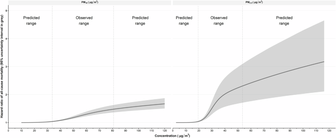
SCHIF, shape constrained health impact function. Hazard ratios for PM10 and PM2.5 were predicted using the expectation of the posterior distribution from the Bayesian modeling framework. As shown in Table S1, the observed range for PM10 varied from 33.69–80.84 (mu g/{m}^{3}), whereas the observed range for PM2.5 varied from 19.50–53.48 (mu g/{m}^{3}). Based on the SCHIF, the curves of hazard ratios were extended to cover the predicted range of concentration levels.
Mortality estimates attributable to PM exposure
In Guangdong, the average age-standardized mortality rates attributable to PM2.5 exposure dropped from 3807.72 (95% UI: 3293.60–4324.34) per million to 484.50 (95% UI: 409.36–567.76) per million, with a mean annualized rate of -9.35% (95% UI: -9.64, -9.06), avoiding an annual number of 0.193 (95%UI: 0.175–0.212) million mortality cases. Table 1 presents the age-standardized PM2.5 attributable mortality burden by city and age. The top three cities carrying the heaviest attributable burden changed from Shaoguan, Chaozhou, and Foshan in 2000 to Meizhou, Chaozhou, and Dongguan in 2021. The age-standardized mortality attributable to PM10 is shown in Table S4, with Chaozhou and Dongguan generally ranking at the top in 2021.
Potential gains in LE due to the reduction of PM
In the total population, the average LE increased from 73.95 years (95% UI: 70.53–79.98) to 77.24 years (95% UI: (73.57–83.85), with a steady average annualized rate of 0.21% (95% UI: 0.19–0.22). In the scenario analyses, the average gains could reach a respective level of 0.33 (95% UI: 0.28–0.38) and 0.58 (95% UI: 0.49–0.67) years for the 5.6% and 10% reduction scenarios. In the scenario implementing the new WHO guidelines, the overall gain in LE could be averaged to 4.07 years (95% UI: 3.60–4.52). Figure 3 further demonstrates the potential LE gains that can be attributable to different magnitudes of reduction in PM2.5. If the PM2.5 reduction level in the prefectural city reaches, for instance, 45.0 (mu g/{m}^{3}), the pollution reduction would monotonically yield an increase of 5.78 years (95%UI: 5.04–6.55) in LE. Scenario analyses for PM10 reduction are shown in Figure S7, with similar trends but smaller LE gains. At the prefectural level, meeting the WHO guidelines would yield an overall increase of 5.36 years (95% UI: 4.72–5.99) in LE for Chaozhou, which was then followed by Foshan and Shaoguan (Fig. 4). Estimates of PM10 show similar patterns of LE gains, but the values of gains were comparatively lower (Figure S8).
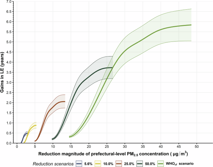
Potential gains in life expectancy in Guangdong, with five reduction scenarios for the exposure to ambient PM2.5. LE, life expectancy; ({{WHO}}_{{cf}}), the counterfactual exposure level. Shaded areas reflected the variation of LE gains across all prefectures. The x-axis reflects the magnitude of concentration reduction, given the observed range of PM2.5 levels during the study period. The non-linear trends were plotted using the Bayesian posterior draws.
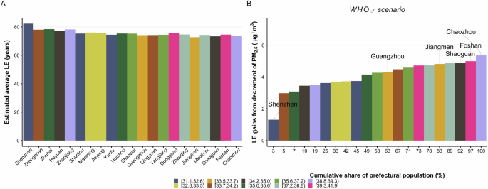
LE, life expectancy; ({{WHO}}_{{cf}}), the counterfactual exposure level. Panel (A) shows the estimated average life expectancy by prefecture while panel (B) shows the potential gains in average due to the reduction to the new WHO guideline levels. The color legend indicates the observed annual mean PM2.5 concentrations during the study period in Guangdong, and was presented as 10-group categories.
Discussion
While there is a substantial body of evidence supporting the causal link between high levels of PM and mortality13,18,19, our refined understanding of the shape function represents one of the few attempts to examine the health benefits associated with the implementation of the latest WHO guidelines in China. By quantifying the health impacts using LE, we estimated that PM reduction till the ({{WHO}}_{{cf}}) level could lead to an average gain of 4.07 years. Interestingly, a PM2.5 reduction level attaining over 45 (mu g/{m}^{3}) may even contribute to a total of 5.78 years in LE gains. These findings provide a clearer path for extending the population’s life span and promoting sustainable development. Besides, the largest regional cohort of over 0.58 million people in our study ensures sufficient statistical power to detect the age-specific effects of PM on mortality and the generalizability of the findings15. With a comprehensive assessment framework, the current study highlights the need to accelerate the development of environmental public health policies beneficial to LE gains. To implement the best scenario for reducing PM pollution, extensive efforts from governments, policymakers, and other relevant stakeholders are required.
We observed a sigmoid shape of the relationship between PM and the risk of all-cause mortality, with magnitudes and shapes resembling those previously reported4,5,19,20. Firstly, our effect estimates were somewhat comparable to what has been reported in European regions and China. For instance, Strak et al.2 reported an ensembled HR of 1.30 [95% confidence interval (CI): 1.14–1.47] per 5-unit increase in PM2.5 among the European pooled cohorts, while Li et al.19 found an HR of 1.08 (95% CI: 1.06–1.09) per 10-unit increase in the PM2.5 range of 40–113 (mu g/{m}^{3}) among the elderly Chinese population. These studies have overlapping uncertainty intervals with our findings. In contrast, our estimates were higher than those reported by Pappin et al.4, who estimated an overall HR of 1.053 (95% CI: 1.041, 1.065) per 10-(mu g/{m}^{3}) among the entire Canadian cohort. Notably, our estimates for PM2.5 ranging below 15 (mu g/{m}^{3}) were significantly lower than those reported from the United States Medicare cohort (1.073, 95% CI = 1.071–1.075)5. The underlying differences subtly imply the possible effects of low PM on all-cause mortality, but future studies shall be warranted when actual information on lower PM levels is available. Nevertheless, the uncertainty interval of the relationship, particularly at the higher PM level, largely overlaps with the non-linear function previously reported by the other Chinese cohort studies13,19. This comparison may suggest a degree of consistency with prior publications regarding the shapes. On the one hand, the shape function may play a crucial role in the health benefits assessment of PM control strategies and policies. With a wide range of PM concentrations across the shape function in regions with varied levels of pollution, the issue of attributable mortality burden and potential loss of LE may still be emerging. We believe this, would in turn, has a marked impact on the policymaking targeting environmental public health and population longevity. In particular, the wide range of PM concentrations in the study region and also in the other parts of China presents even greater policy and technological challenges compared to those faced by European and North American regions. The rationales are twofold. First, reducing and maintaining the annual mean concentrations at relatively low levels would require substantial green economic investments and consistent technological reforms21,22, which may not be universally affordable in local areas. Second, attaining this PM reduction target would require extensive efforts and collaboration among various authorities and multiple sectors to develop and enforce stringent air quality policies23,24. Yet, the priority of extending life expectancy through PM reduction may sometimes conflict with the goal of economic development.
Our findings reveal the same positive trends between PM reduction and gains in LE, which are consistent with those previously reported11,16,25,26. For instance, Zheng et al.11 reported a 10% reduction in PM2.5 would result in a 38.4-day increment in LE; Wu et al.16 found a 10-(mu g/{m}^{3}) decrease in PM2.5 was associated with an increase of 0.18 year in LE among the urban population; and finally, Tsai et al.26 estimated a 10-(mu g/{m}^{3}) decrease could yield a 0.197 year increase in LE. Indeed, our estimated increases in LE are higher than those from these previous studies. The rationale for the difference can be attributable to two factors. Tsai et al.26 and Wu et al.16 used the direct regression approach and neglected age-specific effects as well as the non-linear effects. As a result, this may lead to an underestimation of LE gains in different age groups and in areas where PM pollution is reduced from a higher level. Secondly, Zheng et al.11 failed to consider the regional-specific mortality rate and implemented the national average mortality rate instead. This modeling strategy may lead to an underestimation of city-level LE, particularly in cities with lower all-cause mortality rates. Nevertheless, the comparable magnitude supports our approach of calculating age-specific effect estimates and attributable burden of disease, which is an important component highlighted in our study. Altogether, these findings offer new insights into the estimation methodology of LE gains due to PM reduction.
Moreover, the multi-scenario analyses demonstrate the additional health benefits achievable through various PM2.5 reduction strategies. While the 5.6% and 10% reduction scenarios align with the current policy, these reduction targets may only result in trivial gains in LE, typically no more than 1 year. In contrast, the more stringent reduction scenario incorporating the latest WHO guidelines suggests a higher level of LE gains. This finding is comparable to the LE gains reported by Lelieveld et al.27. More importantly, the assessment of the ({{WHO}}_{{cf}}) scenario may provide concrete guidance for the achievement of the LE goal outlined in the Healthy China 2030 plan28. Although Guangdong has almost achieved the 2020 goal, attaining a level of 77.24 years, there remains a considerable distance to go before reaching the 2030 goal of 79.0 years. With both PM2.5 reduction measures and sustained efforts maintaining the average annualized rate of gains, it might be likely that the overall LE would reach 78.71 years. This would leave a gap of 0.29 years closing to 79.0 years. These anticipated results urge the government and relevant stakeholders to accelerate improving environmental health and invest more resources in areas with higher attributable mortality8,29. Next, we observed consistently monotonical trends in health benefit outcomes for the multi-scenario analyses. These findings can, in part, be explained by the SCHIF curve transition from sublinear to flattening shape at higher exposure levels. The monotonical trends would also suggest a non-linear relationship between PM reduction and gains in LE. To the best of our knowledge, our work is among the first few pieces of research that systematically synthesized evidence regarding this shape, aside from those reported by Correia et al.30 and Yin et al.17. As the Chinese government is committed to the goal of building and maintaining a healthier China, our findings, along with those of Pan et al.31 and Lei et al.32 could serve as crucial evidence for advocating timely synergetic efforts to reduce both the emissions and concentrations of major air pollutants. Importantly, the Clean Air Acts and carbon neutrality may pave a cost-effective roadmap toward achieving this goal. Specifically, the emission sources of air pollutants in Guangdong appear to originate from various means of transportation, heavy industry sectors, and power generation plants32,33. The similarities34 between the sources of PM pollutants and greenhouse gases nevertheless necessitate co-reduction mitigation measures and policies. For instance, the following strategies and measures could positively impact pollution and carbon reduction: transitioning to greener and lower-carbon energy through technological innovation35, promoting clean energy in urban transportation and public services36, imposing tighter pollution emission standards37, encouraging pollution and carbon trading as well as tax policies38, and implementing more comprehensive control measures across industries, power plants, agricultural production, construction sites, and other sectors33,39,40. While Pan et al.31 suggest that synergetic reduction strategies may offset technical abatement costs, admittedly, comprehensive mitigation options remain challenging due to economic development constraints and local policy implementation. Thus, we recommend the authorities and relevant public sector agencies gradually adopt the new WHO guidelines, while thoroughly considering regional economic conditions and resource availability. Although the cost-benefit analysis of implementing the latest WHO guidelines within the framework of the Healthy China 2030 initiative has yet to be conducted, the potential health benefits, including increased longevity due to higher reduction levels of air pollution should not be overlooked.
A distinct strength of the study lies in the incorporation of a regional cohort involving more than 0.58 million individuals from Guangdong. The detailed information on individual covariates, the contextual level variables, and the follow-up status allowed for more accurate detection of the effect estimates across various age groups (Figure S4). In particular, as indicated by our cohort profile41, the demographic characteristics of the enrolled participants remained comparable to those of the general Guangdong population. While the enrolled participants were somewhat healthier than the broader population in terms of lifestyle factors, the prevalence of major chronic diseases was consistent with that of the general population, as indicated in several previous studies42,43,44. The regional representativeness of the Pearl River Cohort study, combined with the systematic modeling framework, may enhance the potential generalizability of these findings to other areas facing similar environmental challenges and air pollution patterns worldwide. Another key strength is our comprehensive framework, which enables us to capture the potential influences of age, the variation of concentrations, and the non-linear trends between PM reduction and LE gains. Lastly, previous comparative risk assessments rely mostly on pre-built SCHIF models such as the integrated exposure-response model7,45 and the original GEMM11,27,46. These models are primarily synthesized based on foreign cohorts conducted at the country level. Questions remain about whether they can be directly applied to the local settings with high air pollution47. In contrast, we performed the SCHIF parameter estimation based on information extracted from our regional cohort (Table S3). Specifically, we accounted for the baseline status and time-varying annual air pollution levels in the Cox model following the implementation of Clean Air Acts initiated in 201348. Consequently, the model estimates may capture the health impact of the drastically declining annual mean PM concentrations experienced by our cohort participants (Fig. 1). These methodological strategies can be extended to other types of air pollutants, such as various mixed PM components, while the modeling framework would serve as a reliable foundation for further investigation of the health impact of these pollutants in other regions of the world.
A few limitations should be noted. First, we assigned PM exposure based on residential addresses, an exposure assessment strategy widely used in previous environmental health studies17,49. However, this approach may lead to unavoidable measurement bias50. Such bias could result in an underestimation of the all-cause mortality burden attributable to PM exposure, despite our efforts to integrate the highest spatial resolution dataset available into our modeling framework to minimize the potential impact of these biases51. Second, we did not consider source-specific effect estimates, e.g., active smoking, secondhand tobacco smoke, etc. The inclusion of source-specific effects is a feature emphasized in the integrated exposure-response model7,45 but omitted in the GEMM due to the high variance of source-specific effects14. However, as suggested by our prior study52, the effect estimates yielded by the GEMM modeling framework were generally larger than those from the integrated exposure-response model, with seemingly wider uncertainty levels at higher PM exposure levels. Additionally, in the sensitivity analyses (Figures S5 and S9), the exposure-response relationships remained robust and consistent, even after adjusting for ozone, smoking, and drinking. Therefore, our modeling framework may still be capable of deriving consistent estimates despite omitting the underlying source-specific variance. Finally, data on cause-specific and gender-specific mortality were not available from the Statistical Yearbook or population census reports. Nonetheless, our findings still serve as a novel piece of evidence unveiling the possible health benefits of reducing PM to a level below the existing Chinese standards.
In conclusion, this comparative risk assessment study identifies a sigmoid shape function for the relationships between PM and all-cause mortality and between PM reduction and life expectancy gains. The risk assessment of PM exposure should be framed in the context of non-linear evaluation. By implementing the 2021 WHO air pollution guidelines, additional LE gains may be attained, which outlines a clearer sustainable path for attaining the Healthy China goals. This study also emphasizes the need to tailor targeted strategies and public health policies that could optimize LE, promote environmental health, and foster socioeconomic prosperity and wellness.
Methods
Analytical Cohort
We used the Pearl River Cohort data collected by the Major Projects of Science Research for the 11th (2006–2010) and 12th (2012–2017) five-year plans of China, involving over 0.58 million subjects in Guangdong, China. Briefly, the community-based cohort comprises healthy participants recruited through a multistage, stratified cluster sampling method. The baseline investigation was conducted from 2009 to December 2015, after which a follow-up survey was performed during 2018–2020 to keep track of participants’ survival status. Information on social-demographic variables (i.e., birth date, sex, marriage, education, body-mass index, residential address, etc.) was available and medical records on all-cause mortality were extracted from the death registration system provided by the Guangdong Provincial Center for Disease Control and Prevention. Written informed consent was obtained before enrollment. The study was approved by the Ethics Committee of Sun Yat-Sen University. Details on this analytical cohort have been described elsewhere15,41,53.
Ambient air pollution and auxiliary covariates
We used pollution data extracted from Tracking Air Pollution in China (TAP) at a 0.01°(times)0.01° resolution ( ~ 1 km2) over the study region for 2000–2021. Daily pollution data including particulate matter (PM10) and fine particulate matter (PM2.5) were available in this well-established high-coverage database, which has been extensively used in previous studies54,55,56. Annual PM averages were calculated from daily concentrations and assigned to each participant by residential address and by each year of the cohort follow-up, following the previous publications49.
We extracted auxiliary covariates from various other sources. For the time-varying meteorological variables (i.e., temperature, °C; precipitation, mm, etc.), we used the monthly TerraClimate database, which is a global gridded database with a resolution of 4 km. For the contextual risk factors, we considered the socio-demographic variables including disposable income per capita (RMB), average duration of education (years), and natural birth rate (‰). These variables reflect the total quality of life among the population57. Details concerning the data source and estimation method of the socio-demographic index can be found in Table S158,59. The all-cause mortality rates, residential population, and city-specific age structure were extracted from the Statistical Yearbook and population census reports. Details about these can also be found in Table S1.
Statistical analysis
Our primary model linking PM to all-cause mortality was the time-varying Cox regression60, where the potential temporal variation in exposures was considered. We defined the event of interest as the all-cause mortality while considering any cause of death. The mortality outcome was validated via linkage to the death registration system. Following a prospective cohort design, we fitted models with reference to our a priori directed acyclic graph15 and included age, sex, marriage, education, and the penalty spline of the body-mass index as the initial predictors. We further considered temperature and precipitation in the main Cox model (Figure S4). The auxiliary covariates were examined by Spearman’s correlation analysis and the variance inflation factor to control for potential influences of collinearity (Table S2). Alternative to the minimal sufficient adjustment sets, smoking as well as drinking behaviors and ozone exposure were additionally considered. As suggested by previous publications61,62, these sensitivity analyses may capture the underlying confounders in the relationships between PM exposures and outcomes (Figure S5). The Cox model was then stratified by age (5-year groups). Our study complies with the Guidelines for Accurate and Transparent Health Estimates Reporting (GATHER) statement.
Shape of the relationships between PM and all-cause mortality
In this section, we describe a synthesized shape-constrained health impact function (SCHIF) that captures the concentration-response relationship between ambient concentrations of PM and all-cause mortality. We used the model that linked the logarithm of the baseline hazard function to PM exposure4, (log left(H{R}_{{PM}}right)=theta fleft(zright)omega (z)), where (fleft(zright)=log (((z+alpha )/({{WHO}}_{{cf}}+alpha )))) and (omega left(zright)={left{1+exp left(-frac{z-mu }{nu }right)right}}^{-1}) such that (log left(H{R}_{{PM}}right)=0) for PM concentration ((z)) ranging ([0,,{{WHO}}_{{cf}}]). This constraint feature assumed no effects below the new WHO guidelines (({{WHO}}_{{cf}}), the counterfactual level). Following an a priori assumption about how the hazard ratios of PM varied with age, we smoothed the logarithm of hazard ratios (HRs) using a Bayesian decay function as explained in Figure S4. Based on the smoothed log-hazards of PM and the concentration transformation formula of (fleft(zright)omega (z)), we converted the effect estimates ((theta)) in the SCHIF into a unit scale similar to those reported by the Global Exposure Mortality Model (GEMM)14,27. Specifically, the parameter ((alpha)) models the plateau of the curvature in the (fleft(zright)) function for ({rm{z}} > {{WHO}}_{{cf}}). The parameter ((nu)) controls the curvature of the weighting function4, where large values tend to generate shapes with less curvature and enable the shape to vary between log-linear and linear10. The parameters ((theta), (nu), (mu), and ({rm{alpha }})) were estimated by Hamiltonian Monte Carlo, assuming hyperpriors that yielded reasonable uncertainty for the health benefits analysis (shown in Table S3). Finally, we defined the counterfactual level at ({{WHO}}_{{cf}} sim {Uniform}(10,,15)) for PM10 and ({{WHO}}_{{cf}} sim {Uniform}(2.5,,5)) for PM2.5, separately, following a prior study in Canada9 and the WHO guidelines1.
Decomposition of prefectural-level all-cause mortality by age
We implemented the Bayesian hierarchical models with fixed effects on time and the socio-demographic index (Figure S6), plus nested random effects by region and city, against the logarithm of the all-cause mortality rate. We also considered the random slope for the socio-demographic index across time (shown in Figure S1). We then predicted the city-level log-mortality rates based on the modeling posterior distributions. After which, we decomposed the all-cause mortality rates into a total of 19 abridged age groups (i.e., 0 ~ , 1 ~ , 5 ~ , 10 ~ , …, 85 + ), following the age spline models used in the Global Burden of Disease study58,63. We further adjusted for the non-linear trends due to mortality under 5 years by implementing the Gaussian Process regression64. Details on the procedures and the grouping of regions can be found in the appendix (I–II).
Risk-eliminated life expectancy and uncertainty analysis
We quantified the health impacts of reduced PM concentrations by using the life table method. Firstly, we used the hazard ratios estimated from the SCHIF of the cohort (Figure S4) and the distribution of PM in the population by city to calculate the attributable fraction ((A{F}_{{weighted}}), as shown in the appendix Section III). Next, we calculated attributable mortality using ({Attributable; mortalit}{y}_{{by; age}}={mortalit}{y}_{{by; age}}times A{F}_{{weighted}}) and derived the risk-eliminated LE by subtracting the attributable mortality probability from the standard mortality probability equation. Based on the SCHIF, we considered 4 additional scenarios for PM reduction (with reduction rates being set at 5.6%, 10%, 25%, and 50%), as alternatives to the ({{WHO}}_{{cf}}) scenario. For the uncertainty analysis, we used draw-level estimates extracted from the posterior distribution and computed the 95% uncertainty intervals (UI) at the 2.5% and 97.5% percentiles. Analyses were conducted in R (version 4.0), with the brms packages.

Responses