How much longer do you have to drive than the crow has to fly?

Introduction
The development of a transportation network is an iterative process driven by the need for easy accessibility. In urban areas, streets are built to connect locations already in place, but the site selection for hospitals, shops, warehouses, etc., is influenced by the existing street network1,2,3. This also applies, mutatis mutandis, to the construction of the motorway networks which began about 100 years ago or later, depending on the country, after a certain level of industrialisation had been reached. But the socio-economic benefits4,5,6 of a transportation network in a given country cannot grow indefinitely with the network’s further enlargement. Construction of new motorways is costly and criticised in modern societies for environmental and other reasons. There is a kind of diminishing marginal utility.
The question arises as to how to quantitatively characterise this trade-off between conflicting interests. Of course, a general answer must involve a large variety of aspects, ranging from engineering and geographical matters to economic and demographic considerations to environmental and political issues. Here, we want to contribute to an answer by putting forward an approach that is based only on the motorway network itself, more specifically, on statistical properties of two kinds of distances.
To measure accessibility in a transportation network, a natural observable is the distance between locations1,7. The distance in a transportation network is measured by searching the shortest path on the network between two locations. This defines the network distance, which is distinct from the Euclidean and the geodetic distances between the same locations. For urban areas or, more generally, for a moderate extension of the network, the Euclidean distance suffices, but it should be replaced by the geodetic distance if the curvature of the Earth becomes relevant8. These two distances ignore changes in elevation. The network distance includes curvature as well as elevation effects; the latter should be relatively small for the motorway networks in most countries.
Comparing the network and the Euclidean or geodetic distances gives information on accessibility in a transportation network. Various studies have been put forward. Correlation and regression analyses9,10,11,12 were employed to quantify the network efficiency. Improved search methods in spatial databases13 were proposed. The ratio of network and Euclidean distances is often referred to as detour index or circuity. Slope and straightness centrality are related quantities whose distributions were investigated in refs. 14,15. Importantly, these studies are devoted to transportation on smaller scales or in metropolitan areas. In the context of urban data, various kinds of scaling behaviour were identified, e.g., for urban spatial structures16,17, urban supply networks18 and urban road networks19,20. Scaling properties shared by the distributions of urban and cropland networks21 were identified. The scaling behaviour is often related to network distances22,23 or to the detour index24.
The scaling that the majority of the previous studies focus on is between network and Euclidean distances mostly in urban regions, leaving aside the non-urban regions. Thus far, empirical information and comparisons of the network and geodetic distance distributions for motorway networks covering urban and non-urban regions have not been offered. Motorway traffic features high driving speed, high traffic flow, an absence of traffic signal control, etc., distinguishing it from traffic on urban or other transportation networks. Here, we have three goals: first, we present a thorough empirical analysis of network and geodetic distance distributions for a variety of countries and larger areas with different geographic, topological, economic and political conditions. Second, we identify a surprisingly uniform scaling between the two distributions with remarkable stability observed in different countries. Third, by comparing simulated networks, we present strong evidence that this scaling is due to the presence of guiding principles rather than randomness in the development of a motorway network. We substantiate this by providing a set of rules that mimics realistic motorway networks, which is related to but different from other models as in refs. 8,25,26,27.
Results
Data analysis and empirical results
To begin with, we choose the motorway networks in China, France, Germany, Spain and the contiguous part of the United States of America, i.e. the US excluding Alaska and Hawaii, see Fig. 1a–e. All motorway network data are provided by OpenStreetMap (OSM). For each network, we select around 2000 locations on motorways. To account for network connectivity, we work out the network distance l(n) and the corresponding geodetic distance l(g) between each pair of locations if there is a path between them. The empirical results for the two probability density functions (pdf) or distributions p(n)(l) and p(g)(l) are shown in Fig. 2a. When the distances appear as arguments, we drop the upper indices g and n. When we compare the different motorway networks, the scales and shapes differ as is to be expected. However, when we compare the two distributions for a given network, we find that the scaling property
is realised in a good approximation. The scaling factors α are empirically determined by minimising the residual sum of the squares ({({p}^{{rm{(g)}}}(l)-alpha {p}^{{rm{(n)}}}(alpha l))}^{2}). As displayed in Fig. 2b, the distributions almost fully agree after rescaling p(n). We obtain values of α between 1.2 and 1.5. For comparison, ref. 28 found a factor of 1.18 between network and Euclidean distances for US inter-city road networks by considering cities as nodes, which is related to but different from the data analysed here. To quantify the similarity of the distribution pairs after rescaling, we use the Hellinger distance H29, see ‘Methods’. It satisfies the property 0 ≤ H ≤ 1, and the better the agreement, the smaller it is. The empirical Hellinger distances in Fig. 2 are quite small, confirming the visual impression. The scaling (1) implies ({langle {l}^{k}rangle }^{{rm{(n)}}}={alpha }^{k}{langle {l}^{k}rangle }^{{rm{(g)}}}) for the k-th moments of the distributions, see Methods. For k = 1, we obtain that the mean network distance is α times longer than the mean geodetic distance. Some features of the distributions can be approximatively understood with a simple analytical model, see Sec. S6 in Supplementary Information (SI).

Motorway networks (black lines) in China (a), France (b), Germany (c), Spain (d), the contiguous United States of America (e), California (f), Great Britain (g), Ontario (h) and North Rhine-Westphalia (i), respectively, with the locations (red dots) used to calculate distances. Motorway network data provided by OpenStreetMap (OSM) © OpenStreetMap contributors35,36. Maps developed with QGIS 3.437.
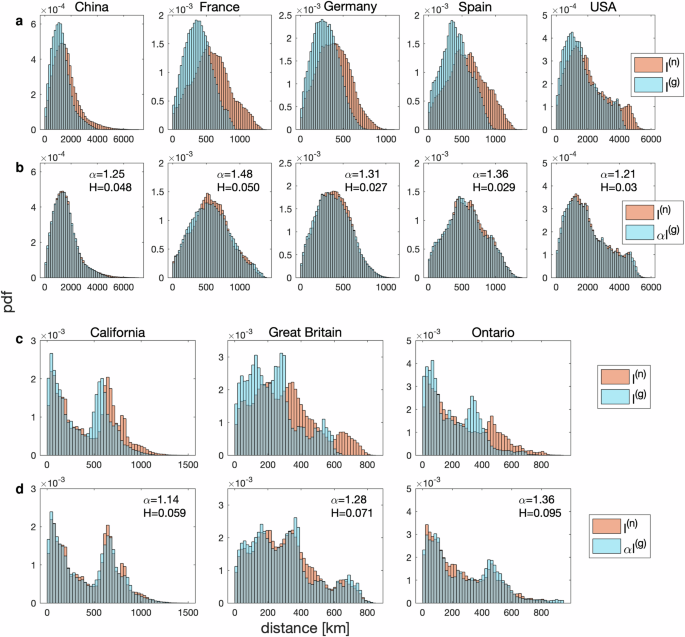
Distributions or pdfs p(n)(l) and p(g)(l) of network and geodetic distances for the eight motorway networks in Fig. 1, before (a, c) and after (b, d) scaling. Scaling factors α and Hellinger distances H are given in the subfigures of (b) and (d). Grey indicates an overlap of two distributions.
Is the scaling property due to the relatively homogeneous structure of the motorway networks we examined? This is not so, as the analysis of the networks in Great Britain, i.e. the United Kingdom excluding Northern Ireland, California, USA, and Ontario, Canada, see Fig. 1f–h, reveals. The topology of the networks is bimodal for California and Ontario, and even trimodal for Great Britain, resulting in distributions very different from the previous ones, as depicted in Fig. 2c. Remarkably, the scaling property is still present, see Fig. 2d. We obtain values of α between 1.1 and 1.4, slightly lower than the ones above because the network and geodetic distances between locations in different centres of the multimodal networks tend to be close. Despite the rich structures of the distributions, the Hellinger distances H are small, see Fig. 2. Hence, the scaling behaviour is, at least in the cases considered here, independent of the network topologies.
Does the scaling property require a relatively large motorway network? Not surprisingly, there is such a tendency, but in Sec. S2 of SI, we present an analysis of the motorway networks in the 16 German states which reveals a remarkable robustness. Even the smaller states show approximate scaling, but typically with larger values of α and H.
Is the scaling behaviour robust when we modify the randomly chosen set of locations? To study this, we take a closer look at North Rhine-Westphalia (Nordrhein-Westfalen), see Fig. 1i, the most populous German state, with its large motorway network. As Fig. 3b, c shows, the scaling is very well developed. We now randomly select other sets of 2000 locations each and find only slight changes in the scaling factor α and Hellinger distance H. We also vary the number of locations in the chosen sets, up to 10,000, and do not see a significant change in α and H either, see Sec. S3 in SI. Hence, the scaling is no coincidence; rather, it is a robust feature of large motorway networks.
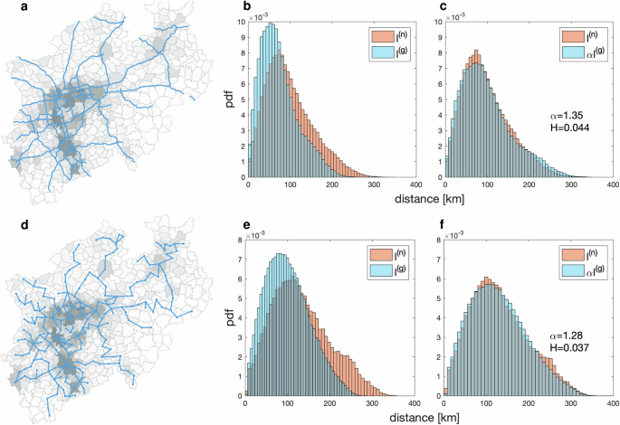
a Real motorway network and d constructed region motorway network for North Rhine-Westphalia. Distributions p(n)(l) and p(g)(l) of network and geodetic distances before (b, e) and after (c, f) scaling. b, c These are for the real motorway network. e, f These are for the constructed region motorway network. In (a, d), the underlying grey colour indicates population density; the darker the colour, the higher the population density. Data on motorway networks (blue lines) and region boundaries (light grey lines) provided by OpenStreetMap (OSM) © OpenStreetMap contributors35,36. Population density data, licensed under BY-2.038, provided by © Statistische Ämter des Bundes und der Länder, Germany39. Maps in (a) and (d) were developed with Python40.
Types of networks and scaling
Which properties must a motorway network have to be realistic—in particular, to exhibit scaling? We tackle this question by studying network models. A real motorway network connects locations. A network model consists of nodes and edges to which we in the present context refer as locations and motorways, respectively. We will work out the network and geodetic distances between the locations. We choose an area of ~550 km × 550 km, roughly corresponding to the sizes of the European countries and areas analysed empirically. Let us begin with the simplest network, a fully random one, by randomly selecting n locations, such that there are N = n(n − 1)/2 possible motorways between them. Given n locations and a connection fraction f we randomly choose fN motorways, see Fig. 4a, for example. If two locations are connected by a path in the motorway network, we work out the geodetic and the shortest possible network distances. Figure 4b, c displays the distributions of the two kinds of distances before and after scaling, respectively, taking f = 0.2 and n = 100 as an example. As seen in Sec. S4.1 of SI, the corresponding distributions for n = 100 strongly depend on the value of f. For smaller f ≤ 0.3, the shapes are so different that scaling is absent, as revealed by the large Hellinger distances H > 0.1. For f ≥ 0.4 onwards, the distributions begin to coincide trivially with α = 1. This behaviour does not match the empirical findings. In the real world, a motorway connecting two locations would not avoid a location in between and close by. Thus, the fully random motorway network contains a high number of unrealistic motorways, which alters the statistical features. We infer that in a better motorway model, neighbouring locations ought to be connected. A good model with that feature is a random grid network, see Fig. 4d, for instance. In the above specified area, we choose a 30 × 30 grid of locations at regular intervals, and only allow motorways connecting adjacent locations in any direction, including diagonally30. Motorways in this model do not cross. According to a fraction f, we then select locations to be connected. When f = 0.2, the scaling behaviour for distance distributions is absent for H > 0.1 in Fig. 4e, f. As shown in Sec. S4.2 in SI, the motorway network consists of unjoined parts which grow together beyond f = 0.3 or so. Apart from strong discrepancies for very small f, the distributions for f > 0.3 show some scaling with higher values of α and differing in the details, but corroborating the above reasoning. Furthermore, we examine random spatial networks with locally finite configurations, including random geometric networks and K-neighbour networks based on randomly selecting n locations28,31,32, see Secs. S4.3 and S4.4 in SI, respectively. For the former, we connect two locations if their geodetic distance does not exceed a threshold. For the latter, we connect two locations if a location belongs to the K closest neighbours of the other. The two kinds of networks are obviously local regarding the connections, see a random geometric network with f = 0.2 in Fig. 4g. The case of K-neighbour networks is analogous. The corresponding distributions of network and geodetic distances in Fig. 4h are indistinguishable, resulting in a scaling factor of α = 1.01, see Fig. 4i. This considerably differs from our above empirical findings for real motorway networks, which demonstrates that the two kinds of spatial networks are unable to describe the realistic motorway networks. The locality of network connections appears not to be the decisive feature.

a Fully random networks with n = 20 locations and connection fractions f = 0.2. Distributions p(n)(l) and p(g)(l) of network and geodetic distances before (b) and after (c) scaling for fully random networks with n = 100 locations and f = 0.2. d Random grid networks with 64 locations on an 8 × 8 grid and f = 0.2. Distributions p(n)(l) and p(g)(l) of network and geodetic distances before (e) and after (f) scaling for random grid networks with 900 locations on a 30 × 30 grid and f = 0.2. g Random geometric networks with n = 100 locations and connection fractions f = 0.2. Distributions p(n)(l) and p(g)(l) of network and geodetic distances before (h) and after (i) scaling for random geometric networks with n = 100 and f = 0.2.
Guided by these observations, we now set up a model that realistically mimics features of the North Rhine-Westphalia motorway network. In a real motorway network, see Fig. 1i, the intersections are the nodes, but it would be insufficient to only consider those as locations. In the empirical analysis, any point on the motorway network can be the origin or destination of a journey. Moreover, the model can only be realistic if it is capable of realistically developing a motorway network. A real motorway network connects cities, districts, municipalities, etc., see Fig. 3a, to which we refer as regions. They will serve as possible locations, but not all of them will be connected. The importance of a region largely depends on the number of inhabitants. The North Rhine-Westphalia motorway network has no unjoined pieces, prompting us to require that only adjacent regions be connected. To promote accessibility, more populous regions are connected by motorways, even if they are not adjacent. Hence, less populous regions in between become connected, but not all regions, adjacent or not, are connected by motorways. In North Rhine-Westphalia, most motorways are in the most populous area, the Rhine-Ruhr region. The challenge is to specify the regions using published data, and then to convert the existing motorway network to a model network with nodes placed in the centres of these 396 regions, see Fig. 3d. We connect the regions by hand to obtain the best possible match with the real motorway network. When we compare the distributions of network and geodetic distances of the real and the region motorway networks, we find a sufficient match and some differences in the details, see Fig. 3b, c, e, f. The scaling factors and Hellinger distances are α = 1.35, H = 0.044, and α = 1.28, H = 0.037, respectively. It is very important that the region motorway network allows us to determine a connection fraction; we find f = 0.2214 for North Rhine-Westphalia.
A realistic network model for motorways
We can now provide rules for the realistic planning and construction of motorway networks. To the best of our knowledge, there is no such model in the literature. We put forward a partially random network model based on the above findings. The remaining randomness lies in the selections of regions and connecting motorways, allowing flexibility. We will then apply it to North Rhine-Westphalia. For a given connection fraction f, we construct the model network G of m motorways using the following procedure:
-
1.
Construct a fully connected network Gall of n regions and mall motorways without crossings.
-
2.
Randomly select a pair of regions with a selection probability ωij to be specified below.
-
3.
Search the shortest path with length denoted by sij between this pair i and j of regions in Gall, where sij is the sum of the geodetic distances ({l}_{kl}^{{rm{(g)}}}) of all the adjacent regions k and l connected by the path being considered. In the first application of this step, these resulting motorways between the adjacent regions k and l are taken as the first motorways in G. In the later reiterations, only those motorways which are not yet in G are added to G.
-
4.
Reward if a motorway already exists in G by effectively shortening the corresponding ({l}_{kl}^{{rm{(g)}}}) in Gall according to ({l}_{kl}^{{rm{(g)}}}leftarrow {l}_{kl}^{{rm{(g)}}}{varepsilon }_{ij}). The parameter εij is between 0 and 1 and will be specified below.
-
5.
Repeat steps 2 to 4 until the number of motorways m in G reaches m ≥ int(fmall), where int returns the integer closest to its argument.
-
6.
For m > int(fmall), randomly remove a motorway that connects a region which connects only to one other region. Repeat removing edges one by one until m = int(fmall).
We now apply this model to North Rhine-Westphalia. The n = 396 regions are connected by mall = 1084 motorways to form Gall, see Sec. S1 in SI. We use the connection fraction f = 0.2214 obtained above to calculate the number of motorways m in the region network G, m = int(fmall) = 240. As the population densities Pi of the regions i play a crucial role in the topology of the motorway network, we choose the selection probability
which follows an exponential distribution. Paths are searched between regions i and j only if they are chosen according to ωij, and not considered otherwise. It is also useful to relate the updating parameter εij to the population densities,
follows a log-normal distribution. For εij = 0, the distance ({l}_{kl}^{(g)}) in the previously chosen path becomes zero, such that the shortest path for the next region pair must pass through the adjacent regions k and l instead of choosing a path shorter than the original ({l}_{kl}^{(g)}). Thus setting εij = 0 results in a minimum spanning tree. On the contrary, letting εij = 1, a shorter path will replace the connection between k and l ignoring the significance of the region, which generates more loops in the network. Our setting in Eq. (3) is a realistic compromise between the two extremes. The choice of εij favours the additional generation of paths in G that run somewhat parallel to existing paths for densely populated regions while preventing this for sparsely populated regions. Such behaviour is observed in real motorway networks. This model captures salient features of the region motorway network for North Rhine-Westphalia, as we now demonstrate.
A crucial feature of our partially random motorway network is the adjacency, deeply rooted in the above rules, that produces fully connected networks rather than a network of unjoined pieces. For different connection fractions f, we present such modelled partially random motorway networks in Fig. S12 of SI. For comparison, Fig. S14 in SI depicts fully random motorway networks for the same connection fractions f, generated by randomly selecting motorways from the fully connected North Rhine-Westphalia region network, see Sec. S1 in SI, avoiding motorway crossings. We display the distributions p(n)(l) and p(g)(l) of network and geodetic distances in Figs. S13 and S15 of SI for the partially and fully random motorway networks in Figs. S12 and S14. In Fig. 5, we compare the two kinds of networks for f = 0.2. Their network structures as well as the corresponding distributions differ quite a bit. Unlike fully random networks and random grid networks, the partially random networks have distributions very similar to the empirical ones in the real North Rhine-Westphalia motorway network as borne out by lower Hellinger distances, especially when f < 0.4. The corresponding scaling factors are close to our empirical results when 0.2 ≤ f ≤ 0.3. We infer that the very similar scaling properties corroborate that the above set of rules is capable of producing realistic models for motorway networks.
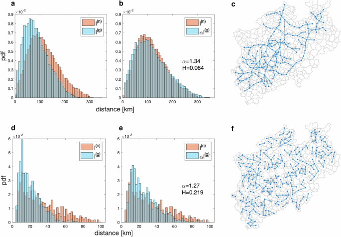
Distributions or pdfs p(n)(l) and p(g)(l) of network and geodetic distances before (a, d) and after (b, e) scaling. a, b These are for the partially random motorway network (c). d, e These are for the fully random motorway network (f). The two networks (c, f) are distributed in the North Rhine-Westphalia region with connection probabilities f = 0.2. Maps in (c, f) were developed with Matlab41.
Discussion
When developing a motorway network, two societal needs are in competition: accessibility and efficiency on the one hand, and cost savings and environmental protection on the other. In an attempt to determine criteria that help to characterise motorway networks in modern countries, we identified a new scaling property that relates the network and the geodetic distances in a remarkably stable manner. We confirm this in a variety of empirical analyses. The extracted scaling factors mean among other things that, on average, the network distance to be travelled is typically 1.3 ± 0.1 times longer than the geodetic distance. This scaling must reflect the aforementioned competition, but it can be analysed on the basis of the motorway networks without additional input. Scaling is best realised in large motorway networks but, surprisingly, even smaller and less homogeneously distributed ones exhibit its onset quite clearly.
We showed that the scaling property is incompatible with simple structures as in fully random networks. Rather, the feature of adjacency is crucial, i.e. real motorway networks develop in such a way that existing connections are most efficiently used. This observation led us to propose a new model: the partially random motorway network, in which motorways grow by connecting adjacent regions step by step. This ensures connectivity. We applied this model to the case of North Rhine-Westphalia, and showed that it reproduces the scaling found empirically very well for the correct connection fraction determined empirically.
In summary, we found a new universal scaling property in motorway networks empirically and, guided by its features, constructed a new, realistic model for such networks.
Methods
Geodetic distance
The geodetic distance between two locations i and j is given by the haversine formula33
Here, φi and λi represent the latitude and longitude of location i, respectively. The Earth’s radius R is approximately R = 6371 km.
Network distance
The network distance ({l}_{ij}^{{rm{(n)}}}) of the shortest path between two locations i and j is measured by combining the tools Osmosis, OSMnx, and NetworkX. Osmosis, a command line of Java applications, is used to filter the geospatial data for a motorway network. OSMnx is a Python package for reading the filtered geospatial data and identifying two given locations separately as an origin and a destination. NetworkX, also a Python package, is employed to search the shortest path between two locations with algorithms, e.g. Dijkstra’s algorithm34 in this study, and to calculate the length of this route only on the motorway network being examined. By exchanging the origin and the destination of two given locations, the distances in the magnitude of kilometres change very little. Hence we use the approximation ({l}_{ij}^{{rm{(n)}}}approx {l}_{ji}^{{rm{(n)}}}). According to the motorway network data provided by OpenStreetMap (OSM) © OpenStreetMap contributors35,36, a motorway connection consists of many, rather small pieces. The length of each edge is close to the geodetic distance ({l}_{ij}^{{rm{(g)}}}) between the two adjacent nodes. Multiple paths may exist for a given pair of locations. The network distance of the shortest path between two locations minimises the sum of geodetic distances along this path. We ignore the network distance if there is no connecting path between two locations. For the general case in our main text, we drop the subscript ij from the distances l(g) and l(n).
Scaling property and moments
The extra factor of α in front of p(n)(αl) in the scaling law (1) follows from the very definition of a pdf. It is needed, for example, to ensure normalisation. The moments with order κ = 0, 1, 2, … of the distributions are
The scaling property (1) for the distributions implies the scaling ({langle {l}^{kappa }rangle }^{{rm{(n)}}}={alpha }^{kappa }{langle {l}^{kappa }rangle }^{{rm{(g)}}}) for the moments with κ = 0, 1, 2, …. Thus, all centred moments and cumulants scale with ακ, too. In particular, the mean value ({langle lrangle }^{text{(z)}}) and the standard deviation scale with α. Here, ({text{var}}^{{rm{(z)}}}={langle {l}^{2}rangle }^{{rm{(z)}}}-{langle lrangle }^{text{(z)}2}) is the variance and ({text{std}}^{{rm{(z)}}}=sqrt{{text{var}}^{{rm{(z)}}}}) is the standard deviation.
Hellinger distance
The Hellinger distance29 of two distributions q1(x) and q2(x) on support X is defined by
By construction, it is zero for q1(x) = q2(x). The Hellinger distance satisfies the property 0≤H≤1. If H approaches zero, the two distributions exhibit a high similarity. In contrast, if H tends towards one, they differ greatly.

Responses