MGNN: Moment Graph Neural Network for Universal Molecular Potentials
Introduction
The computational determination of molecular properties has been significantly accelerated by machine learning. The crux of this advancement lies in the development of machine learning potentials with remarkable efficiency and fidelity. Although the usage of local descriptors in most machine learning interatomic potentials have improved parallel computation and scalability1,2,3,4,5,6, yet they fall short in accuracy compared with atom-centered message-passing neural network (MPNNs) interaction potentials within the concept of graph neural network (GNN)7,8,9,10,11,12, where the molecular systems are treated as 3D graphs, with atoms as nodes linked by edges within a defined cutoff radius. These networks have achieved groundbreaking results, often surpassing traditional models with minimal manual feature engineering. They encode atoms into a high-dimensional space and model interatomic interactions through message passing, effectively serving as surrogates for quantum mechanical simulations7,8,9,10,11,12,13,14,15,16. Machine-learning interatomic potentials have provided promising solutions to bridge the gap between expensive electronic structure methods and efficient classical interatomic potentials17,18,19,20. Most recently, GNN-based machine-learning interatomic potentials trained on the periodic table (for example, M3GNet21 and CHGNet17) have demonstrated the possibility of universal interatomic potentials that may not require chemistry-specific training for each new application17,21,22,23.
In principle, to accurately predict scalar quantities like potential energy, vectorial properties such as forces and dipole moments, and even tensorial properties like polarizabilities24,25,26,27, a GNN which fully accommodates the transformation properties of scalar or tensor is required. For instance, while the translation and rotation of a small molecule do not alter its formation energy, the forces acting on its atoms rotate with the molecule. Most available GNN machine learning potentials address above points by empirically constructing neural network using geometrical quantities like interatomic-distances, bond angles28,29,30,31.
To learn molecular properties satisfying all the needed symmetries, systematical and rigorous routines to treat symmetries are highly desirable. Currently, many machine learning potentials use equivariant message-passing frameworks to achieve such goals, which typically use spherical harmonics as angular basis functions, followed by Clebsch-Gordan contraction to maintain rotational symmetry11,12,32,33,34,35,36,37. However, these calculations are usually expensively. To address such issue, there are emerging efforts on finding efficient computational methods. For instance, a mathematically equivalent and simple message-passing framework that circumvents spherical harmonics is recently proposed, which avoids the usage of high-dimensional Clebsch-Gordan coupling matrix26,38,39. On the other hand, there are a series of mathematical theorems which establishes that the Moment Tensor Potentials4 can provably approximate any regular function satisfying all the needed symmetries, while simultaneously being computationally efficient.
Aiming to develop simple and efficient GNN to learn molecular properties satisfying symmetry requirement, as inspired by Moment Tensor Potential4, we introduce the Moment Graph Neural Network (MGNN), which innovatively propagates information between molecular systems using moments—quantities that encapsulate the spatial relationships between atoms. Our framework defines molecular moments4 to convey relative spatial relationships between atoms within a molecule, utilizing Chebyshev polynomials to encode interatomic distance information instead of more commonly used functions like Bessel and Gaussian radial basis functions28,40. Impressively, MGNN demonstrates multiple state-of-the-art results on benchmark datasets including QM941,42, revised MD1743, and MD17-ethanol44. Its generalizability and efficiency are also tested in additional systems including 3BPA45 and 25-element high-entropy alloys46. Additionally, we demonstrate the high consistency of our framework in predicting molecular dynamics simulations of amorphous electrolytes. Moreover, MGNN’s predictive capabilities extend to the calculation of dipole moments and polarizabilities for organic molecules, such as ethanol, enabling the rapid simulation of molecular spectra in vacuum conditions.
Results
The MGNN architecture
Overview
The Hamiltonian of a molecular system is uniquely determined by the external potential, depending on the charge quantities ({{Z}_{i}}) and atomic positions ({{mathop{r}limits^{ rightharpoonup }}_{i}}). Formally, a molecule in a specific conformation can be represented as a point cloud with (n) atoms denoted as (M=left(Z,Rright)), where (Z=({Z}_{1},ldots ,{Z}_{n})in {{mathbb{Z}}}^{n}) represents the atom type vector and (R=({mathop{r}limits^{ rightharpoonup }}_{1},ldots ,{mathop{r}limits^{ rightharpoonup }}_{n})in {{mathbb{R}}}^{ntimes 3}) represents the atom coordinate matrix.
MGNNs treat molecules as graphs, with atoms as nodes, and edges representing connections between atoms, either based on predefined molecular graphs or atoms connected within a cutoff distance ({r}_{{cut}}). MGNNs represent each atom through atomic embeddings ({h}_{i}in {{mathbb{R}}}^{{H}_{a}}) where ({H}_{a}) is the number of atom features and the edges between nodes (i) and (j) through edge embeddings ({e}_{{ij}}in {{mathbb{R}}}^{{H}_{e}}) where ({H}_{e}) is the number of edge features. These embeddings are updated in each layer through information propagation. In general, the Message Passing Neural Networks (MPNN)14 framework achieves message passing by ({m}_{v}^{t+1}={sum }_{win {mathscr{N}}left(vright)}{M}_{t}left({h}_{v}^{t},{h}_{w}^{t},{e}_{{vw}}right)) and updates by ({h}_{v}^{t+1}={U}_{t}left({h}_{v}^{t},{m}_{v}^{t+1}right)), where ({M}_{t}) represents the message function, ({U}_{t}) represents the vertex update function, and ({mathscr{N}}left(vright)={{w|||}{mathop{r}limits^{ rightharpoonup }}_{{vw}}||le {r}_{{cut}}}) denotes the neighbors of node (v) in graph (G). Our MGNN framework utilizes moment interaction to construct ({M}_{t}) and ({U}_{t}).
In this work, a molecular graph is represented as (G=(A,{E},{T})), where (A) denotes the atoms (nodes), (E) the edges within cutoff ({r}_{{cut}}), and (T) the triplets. Each atom (i) forms an edge with every neighboring atom within its cutoff distance, as demonstrated in Fig. 1a, constructing edges ({ij}), ({ik}), ({im}), and corresponding triplets ({ijk}), ({ijm}), ({ikm}) to formulate the moments. Within a triplet composed of nodes (i,j,k) and edges ({ij}), ({ik}), the message of triplets are used to update edge representation features, which are further used to update node features. As shown in Fig. 1b, for a triplet ({ijk}) whose center is atom (i) and edges are ({ij}) and ({ik}), the information within this triplet first passes to edge ({ij}) (symmetrically to ({ik})), and then the message of edge ({ij}) passes to the central node (i).

a Atom (i) receives information from neighboring atoms (j), (k), and (m) within a specified cutoff radius ({r}_{{cut}}), forming three distinct triplets (({ijk}), ({ijm}), ({ikm})) with (i) as the central atom. b Information flow within a specific triplet ({ijk}), where (i) serves as the central atom and ({ij}) and ({jk}) constitute the connecting edges. c The sequential arrangement of MGNN, from the initial embedding module, through multiple ((N)) interaction layers to the output module. d Architecture of interaction layer, which contains moment interaction layer. e Architecture of moment interaction layer. “Concat” refers to the concatenation of two feature vectors, “CCCP” the continuous cutoff and Chebyshev polynomials-based radial basis function, “Split” the splitting of a long vector into shorter vectors, “(oplus)” the residual connection, “(odot)” the element-wise product, and the dot “(cdot)” in the brackets or follows the “(W)” denotes the input from previous block. See main text for detailed description.
The MGNN framework comprises an embedding block, several sequential interaction layers, and an output block, as shown in Fig. 1c. The molecular charge quantities (labeled as (Z)) first pass through the embedding block to obtain the initial node representation vectors (labeled as (X)). These initial vectors, along with the positions of atoms in Cartesian space containing geometry information (labeled as (R)), are then input into an interaction layer, which uses an interaction block that generates a correction ((Delta X)) to be added to the input ((X)) to generate the current layer output (i.e., (X+Delta X)), which serves as the input for the next interaction layer or output layer. The interaction block (detailed in Fig. 1d) captures how atoms interact with each other, by processing the message from the neighbors of atom (i), during which the interaction between edges from atom (i) (i.e., triplet moment interaction as detailed in Fig. 1e) is involved. There are (N) sequential interaction layers in total. The output after the last interaction layer is labeled as ({X}^{L}), which is then fed into target-dependent output block (detailed in Fig. 2). By aggregating the message of triplets, we construct a comprehensive representation of the molecular structure within the graph, which is then propagated through the interaction layers to update atomic representations. The resulting feature vectors for each atom are fed into the output block, tailored to predict specific properties, culminating in the model’s final predictions. The output module of the MGNN model is adept at generating scalar, vector, and tensor outputs, demonstrating its versatility in capturing and predicting a wide range of molecular properties.
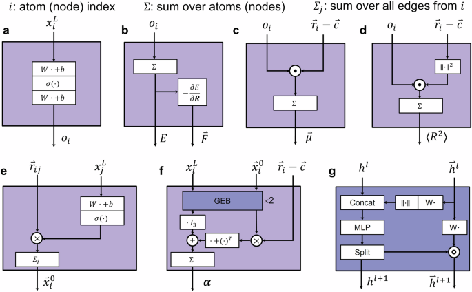
a The MLP block. b The energy and force. c Dipole moment. d Electronic spatial extent. e Vectorial features initialization. f Polarizability, the “GEB×2” denote there are two gated equivariant blocks (GEBs). g The gated equivariant block.
The definition of MLP in current work (as shown in Figs. 1 and 2) is ({MLP}left(xright)={W}^{{out}}left(sigma left({W}^{{in}}x+{b}^{{in}}right)right)+{b}^{{out}}), where ({W}^{{in}}) and ({W}^{{out}}) are learnable weights and ({b}^{{in}}) and ({b}^{{out}}) are learnable biases, and (sigma left(xright)) denotes the element-wise nonlinear activation function. In our experiments, we utilize the SiLU47,48 and Mish49 activation functions. The action of “Concat”, “Reshape”, “Split” in current work (as shown in Figs. 1 and 2) are used to manipulate data dimensions. We use torch.split for “Split” operation. Given a tensor A, suppose the last dimension of A has size 2 F. By performing a split along the last dimension, we can divide A into two chunks, each with a last dimension of size F, while keeping the sizes of other dimensions unchanged. Of course, it’s also possible to split the tensor into other proportions, such as 0.5 F and 1.5 F. for more details, refer to the PyTorch50 documentation. All the notations “(W)” and “(b)” with or without superscript are learnable parameters and we will hint their shape when necessary. Next, we will provide a detailed introduction to each block. The notions employed in this paper are summarized in Supporting Information S1.
Embedding
MGNN works on embedded feature, which is initialized by the embedding block shown in Fig. 1c. Throughout interaction layers, we represent the atoms using a tuple of features ({X}^{l}=left({x}_{1}^{l},ldots ,{x}_{n}^{l}right)), with ({x}_{i}^{l}in {{mathbb{R}}}^{F}) with the number of feature maps (F), the number of atoms (n) and the current interaction layer (l). We maintain a constant number of feature maps at (F=512) throughout the network, if not stated otherwise. The representation of atom (i) is initialized using an embedding depend on the atom type ({Z}_{i},{mathbb{in}},{mathbb{N}}):
The atom type embeddings are learned during training.
Interaction layer
Here we explain the interaction layer shown in Fig. 1c by implementing Eqs. (2)-(13). Within the interaction layer, an interaction block (as depicted in Fig. 1d) produces a correction (Delta X={Delta {x}_{i}}) that is used to update the input embedded feature (X=left{{x}_{i}right}). Formally, the update uses a residual connection inspired by ResNet51, where (l) is the layer index, and ({mathscr{N}}left(iright)) is the neighbor list of atom (i) that determines which edges and angles are involved in message passing.
The residual ({Delta x}_{i}^{l}) is computed through integrating information from edges and angles associated with ({mathscr{N}}left(iright)). For example, for the ({mathscr{N}}left(iright)) shown in Fig. 1a, one angular message is obtained from two edge vectors ({mathop{r}limits^{rightharpoonup}}_{ij}) and ({mathop{r}limits^{ rightharpoonup }}_{{ik}}) originating from node (i) to node (j) and (k) within one triplet ({ijk}), another two angular messages are from triplets ({ijm}) and ({imk}). Since each interaction layer has same structure, for clarity, we no longer indicate the layer index (l) unless necessary.
In one interaction block (as depicted in Fig. 1d), the atomistic representations obtained from the preceding layer (embedding block or previous interaction layer) are passed through a learnable MLP layer:
After updating the atomistic representations using Eq. (3), we concatenate the feature maps of the source and destination nodes of each edge (labeled as ({h}_{i}{||}{h}_{j}) where the symbol “(parallel)” denotes the concatenation of two vectors) to obtain vectors of dimension 2 F. Subsequently, we pass them through a linear layer to convert the feature size of each edge to dimension (beta F), and then reshape them into a matrix ({Phi }_{{ij}}in {{mathbb{R}}}^{Ftimes beta }) (Eq. (4)) and next perform matrix multiplication (Eq. (6)) with a vector ({q}_{{ij}}in {{mathbb{R}}}^{beta }) (Eq. (5)) which encodes the information of ({r}_{{ij}}) using Chebyshev polynomials. The outcome is an edge feature vector ({e}_{{ij}}in {{mathbb{R}}}^{F}) (Eq. (6)):
where (Win {{mathbb{R}}}^{beta Ftimes 2F}) (bin {{mathbb{R}}}^{beta F}).
The ({psi }^{left(beta right)}) in Eq. (5) is the continuous cutoff and Chebyshev polynomials-based radial basis function (“({CCCP}(beta ))” in Fig. 1d), denoted as
Here ({C}^{left(beta right)}) are Chebyshev polynomials on the interval (left[{r}_{min },,{r}_{{cut}}right]), where ({r}_{min }) is the minimal distance between atoms and is usually set to zero, ({r}_{{cut}}) is the cutoff radius which is introduced to ensure a smooth behavior of MGNN when atoms leave or enter the interaction neighborhood. An illustration of the radial basis functions is given in Fig. S1 (Supporting Information S2).
Once the feature maps ({e}_{{ij}}) on the edge are obtained, we split its information (Eq. (8)) to prepare the update on the features of atoms and edges.
where (Win {{mathbb{R}}}^{3Ftimes F}), (bin {{mathbb{R}}}^{3F}), ({Delta}_{{ij}},in {{mathbb{R}}}^{F}), and ({f}_{{ij}}in {{mathbb{R}}}^{2F}). The split information is used to compute the incremental node features as in Eq. (9).
where (Win {{mathbb{R}}}^{Ftimes F}), (bin {{mathbb{R}}}^{F}), and ({xi }_{{ij}}) represents the moment interaction function, as in Eq. (10).
where ({W}^{{in}}in {{mathbb{R}}}^{Ftimes 2F}), ({b}^{{in}}in {{mathbb{R}}}^{F}), ({W}^{{out}}in {{mathbb{R}}}^{Ftimes F}), ({b}^{{out}}in {{mathbb{R}}}^{F}), the symbol “(parallel)” denotes the concatenation of two vectors. ({mathscr{N}}left({ij}right)) represents the set of neighboring edges of the edge ({ij}) that share (i) as a common vertex for all triplets, as shown in the example in Fig. 1b, where ({mathscr{N}}left({ij}right)={{ik},{im}}). Note that applying the non-linearity activation function before aggregation improve performance52.
In Eq. (10), the calculation of ({m}_{{jik}}^{leftlangle nu rightrangle }) (i.e., the message passed by triplet ({jik})) involves the moments that are the core part of our algorithm, as shown in Fig. 1b, e, which are calculated as
where (Win {{mathbb{R}}}^{Ftimes F}), (bin {{mathbb{R}}}^{F}), and “(odot)” denotes element-wise product.
The ({M}_{{theta }_{{jik}}}^{leftlangle nu rightrangle }) in Eq. (11) is the rank (nu) moment of the triplet ({jik}), and is calculated as
where ({hat{r}}_{{ij}}=frac{{mathop{r}limits^{ rightharpoonup }}_{{!ij}}}{{r}_{{ij}}}) is the unit vector of ({mathop{r}limits^{rightharpoonup}}_{{ij}}), ({hat{r}}_{{ij}}^{otimes nu }=underbrace{{hat{r}}_{{ij}}otimes cdots otimes {hat{r}}_{{ij}}}_{{nu ; times}}) is the Kronecker product of (nu) copies of the vector ({hat{r}}_{{ij}}in {{mathbb{R}}}^{3}) and is a tensor of rank (nu). Notation “({{langle }}cdot ,cdot {{rangle }})” signifies the contraction (product) of tensors, with (nu =1) corresponding to the vector dot product and (nu =2) corresponding to the Frobenius product of matrices. In other words, ({M}_{{theta }_{{jik}}}^{langle 1rangle }=langle {hat{r}}_{{ij}},{hat{r}}_{{ik}}rangle =Vert {hat{r}}_{{ij}}Vert times Vert {hat{r}}_{{ik}}Vert times cos (angle {hat{r}}_{{ij}},{hat{r}}_{{ik}})=cos (angle {hat{r}}_{{ij}},{hat{r}}_{{ik}})), and ({M}_{{theta }_{{jik}}}^{langle 2rangle }=langle {hat{r}}_{{ij}}^{otimes 2},{hat{r}}_{{ik}}^{otimes 2}rangle ={hat{r}}_{{ij}}^{otimes 2}:{hat{r}}_{{ik}}^{otimes 2}={cos }^{2}(angle {hat{r}}_{{ij}},{hat{r}}_{{ik}})), reflecting the angular relationship within the triplet ({jik}).
The ({f}_{{ij}}^{leftlangle nu rightrangle }) in Eq. (11) is calculated as
where ({f}_{{ij}}) is calculated using Eq. (8), and ({f}_{{ij}}^{leftlangle nu rightrangle }in {{mathbb{R}}}^{F},,nu =mathrm{1,2}). They serve as the coefficients of moments of edge ({ij}), which will be introduced in next subsection.
The rationale of moment interaction
We get motivation from the moment tensor descriptor4 for atom (i), which is defined as a summation from edge moments as ({sum }_{jin {mathscr{N}}left(iright)}{f}_{{ij}}^{leftlangle nu rightrangle }({r}_{{ij}}){mathop{r}limits^{ rightharpoonup }}_{{ij}}^{otimes nu }), which encapsulated radial part ({f}_{{ij}}^{leftlangle nu rightrangle }({r}_{{ij}})) and angular part ({mathop{r}limits^{ rightharpoonup }}_{{ij}}^{otimes nu }) containing angular information about the neighborhood ({mathscr{N}}left(iright)) and is tensor of rank (nu) 4. Our MGNN defines the moment of an edge ({ij}) as ({f}_{{ij}}^{leftlangle nu rightrangle }({r}_{{ij}},{z}_{i},{z}_{j}){hat{r}}_{{ij}}^{otimes nu }) to account for both ({r}_{{ij}}) and the charges ({z}_{i}) and ({z}_{j}), thereby enriching the function’s capacity to encapsulate the physicochemical context. Note that while ({f}_{{ij}}^{leftlangle nu rightrangle }({r}_{{ij}})) is originally a scalar function of ({r}_{{ij}}) in ref. 4, in MGNN ({f}_{{ij}}^{leftlangle nu rightrangle }({r}_{{ij}},{z}_{i},{z}_{j})) is approximated using neural network.
As the edge moments are contracted to formulate triplet information, edge features (i.e., ({f}_{{ij}}) in Eqs. (8), (9), (11), and (13)) play the role of coefficients to multiply with triplet moment (i.e.,({M}_{{theta }_{{jik}}}^{leftlangle nu rightrangle }) in Eq. (12)) to construct the message passed by triplet (i.e., ({m}_{{jik}}^{leftlangle nu rightrangle }) in Eq. (11)). Within a triplet (i.e., Fig. 1b) composed of nodes (i,j,k) and edges ({ij}), ({ik}), for (nu =1), ({hat{r}}_{{ij}}^{otimes nu }={hat{r}}_{{ij}}), so that ({M}_{{theta }_{{jik}}}^{leftlangle 1rightrangle }=langle {hat{r}}_{{ij}},{hat{r}}_{{ik}}rangle =cos (angle {hat{r}}_{{ij}},{hat{r}}_{{ik}})), and for (nu =2), ({hat{r}}_{{ij}}^{otimes nu }={hat{r}}_{{ij}}otimes {hat{r}}_{{ij}}), so that ({M}_{{theta }_{{jik}}}^{leftlangle 2rightrangle }=langle {hat{r}}_{{ij}}^{otimes 2},{hat{r}}_{{ik}}^{otimes 2}rangle ={cos }^{2}(angle {hat{r}}_{{ij}},{hat{r}}_{{ik}})) (i.e., the Frobenius product). The coefficients ({f}_{{ij}}^{leftlangle nu rightrangle }) and ({f}_{{ik}}^{leftlangle nu rightrangle }) for edges ({ij}) and ({ik}) are derived from Eq. (13).
As can be seen from Eq. (12), all the initial moment tensors are contracted to moment scalars (i.e., zero-order tensors) before the flow of message passing through triplets to edges to nodes, consuming less physical memory in computers. The outputs from message passing are also scalars. When the network is used to predict vectors or tensors, such as dipole moments or polarizabilities, these scalars and geometric information are then used as input formation in the output head to reconstruct vectors or tensors. These are fundamentally different from many existing equivariant models (i.e., GRACE53, and CACE39), where usually the higher-order tensor information is used throughout the entire information flow process.
Output head
When a scalar is needed, the last feedforward network transforms feature on each node into a scalar (Eq. (14)), as shown in Fig. 2a. We perform a sum aggregation over all nodes to predict scalar quantities like energy (Eq. (15)), as shown in Fig. 2b.
The force acting on atoms (i), ({mathop{F}limits^{ rightharpoonup }}_{i}), is computed using auto-differentiation according to its definition as the negative gradient of the total energy with respect to the position of atom (i):
which gives an energy-conserving force field (Eq. (16)), as shown in Fig. 2b44.
The molecular dipole moment (vec{mu }) is the response of the molecular energy to an electric field ({nabla }_{vec{F}}E) and, at the same time, the first moment of the electron density26. It is often predicted using latent atomic charges, and in our model, we predict the dipole moment using Eq. (17) and the electronic spatial extent by Eq. (18), as shown in Fig. 2c, d respectively, consistent with PaiNN26.
This assumes the center of mass at (mathop{c}limits^{ rightharpoonup }) for brevity.
Specifically, when it is necessary to predict properties related to vectors or tensors, a gated equivariant block (for more information about rotational invariance and equivariance, please refer to Supporting Information S5)26,54, as shown in Fig. 2f, is needed. If one needs to calculate the infrared and Raman spectra of a molecular system using deep learning potential functions, it is also necessary to compute the system’s dipole moment and polarizability. In practical experiments, we utilize Eq. (17) to predict the system’s dipole moment. However, to predict the molecular polarizability tensor, we require a vector feature to construct the tensor form. Therefore, we first initialize the node’s vector feature in the output head:
where (Win {{mathbb{R}}}^{Ftimes F}) is the learnable weight used to transform destination node feature to control how much the ({mathop{r}limits^{ rightharpoonup }}_{{ij}}) contributes to the initial node vectorial features. ({x}_{j}^{L}in {{mathbb{R}}}^{F}) is the destination node representation of the edge ({ij}), and the superscript (L) denotes it is the output of the last interaction layer. ({mathop{r}limits^{ rightharpoonup }}_{{ij}}in {{mathbb{R}}}^{3}) is the vector in Cartesian coordinates from source node to destination node. Then through Eq. (19) vectorial features ({mathop{x}limits^{ rightharpoonup }}_{i}^{0}in {{mathbb{R}}}^{Ftimes 3}) of atom (i) can be initialized, in which the superscript (0) denotes the initial vectorial features, as shown in Fig. 2e.
Considering the prediction of polarizability tensor (i.e., the response of the molecular dipole to an electric field26), we construct polarizability tensors using
where ({I}_{3}) is the identical matrix with shape (3times 3), and (mathop{nu }limits^{ rightharpoonup }left({mathop{x}limits^{ rightharpoonup }}_{i}right)) transforms vector features (({mathop{x}limits^{ rightharpoonup }}_{i})) initialized by Eq. (19) and passing them through two gated equivariant blocks26,54, each yielding atom-wise scalars and vectors. The first term describes isotropic, atom-wise polarizabilities. The other two terms are the anisotropic components of the polarizability tensor. The atom positions subtracting the center of mass ({mathop{r}limits^{ rightharpoonup }}_{i}-mathop{c}limits^{ rightharpoonup }) are used here to incorporate the global structure of the molecule26. The calculation of polarizability tensor ({boldsymbol{alpha }}) is illustrated in Fig. 2f and the gated equivariant block in Fig. 2g.
We utilize the open-source deep learning frameworks PyTorch 2.0.150, SchNetPack 2.055, PyTorch Geometric 2.3.156, and PyTorch Lightning 2.1.3 for constructing and training MGNN (see more details in Supporting Information S3). Considering both moment orders (nu =1) and (nu =2), has better performance than considering (nu =1) alone (details in Supporting Information S4).
Benchmark
We show that our MGNN architecture can achieve many state-of-the-art results on QM9 dataset41,42 and some state-of-the-art results on revised MD17 dataset43, and MD17-ethanol44. Furthermore, we validate the stability of MGNN on MD17-ethanol44 and generalizability on 3BPA dataset45 and computational efficiency on dataset 25-element high-entropy alloys57. We refer the reader to the Supporting Information S3 for further training, data set and experimental details.
QM9
The QM9 dataset serves as a widely recognized benchmark for predicting various molecular properties at equilibrium41,42. It comprises 130831 optimized structures with chemical elements (C, H, O, N, F) containing up to 9 heavy atoms (C, O, N, F). In our benchmarking of MGNN, we target 12 properties. To maintain consistency with prior research, MGNN is trained on 110000 examples, while 10000 molecules are reserved for validation purposes to regulate learning rate decay and enable early stopping. The remaining data is allocated as the test set, and results are averaged over three random splits. Table 1 presents a comparison with several state-of-the-art methods that learn the properties described above through a direct mapping from atomic coordinates and species. SchNet28, Physnet31, Dimenet + +40, Equiformer36, PaiNN26, Allegro12, SphereNet58, TorchMD-Net59, and TensorNet38 are included in Table 1 for reference. MGNN attains state-of-the-art performance in seven target properties and delivers comparable results in the remaining targets.
Revised MD17
In our evaluation on the revised MD17 dataset43, which contains 100,000 recomputed structures of 10 molecules from original MD17 dataset44,60,61, we assess MGNN’s capability to accurately learn the energies and forces of small molecules. This dataset comprises ten small, organic molecules, and we aim to predict both energy and forces on systems with fixed chemical composition exhibiting conformational changes. For each molecule, we allocate 950 configurations for training and 50 for validation, uniformly sampled from the entire dataset. Test error is evaluated on all remaining configurations in the dataset. A distinct model is trained for each trajectory. Table 2 presents a comparison with GAP2, ACE5, GetNet-(T/D)29, NequlP(l = 3)11, Allegro12, which are reported in ref. 12, and TensorNet 3L38, BOTNet62, and MACE63 which are reported in ref. 38. MGNN achieves state-of-the-art results for the molecules Ethanol, Benzene, and Uracil, and notably sets a new state-of-the-art for the energy MAE of Ethanol. Furthermore, in other molecular systems, MGNN surpasses previous descriptor-based machine learning interatomic potentials (GAP, ACE), invariant GNNs(GemNet-(T/Q)) or achieves comparable results to other equivariant GNNs(NequlP(l = 3), Allegro, TensorNet 3 L, BOTNet, MACE).
MD17-ethanol
We also benchmark our MGNN in MD17-Ethanol Dataset44, which is frequently used for stability test39,64. Stability refers to the system’s ability to run sufficiently long trajectories while maintaining physically reasonable states. We followed the approach in ref. 39 and used the ethanol molecules in MD17 dataset for training and validation. The models compared include Schnet28, DimeNet30, sGDML65, PaiNN26, SphereNet58, NewtonNet33, GemNet-T29, NequIP11, and CACE39. MGNN-X means that X samples are used to train MGNN. Except for CACE and MGNN-1000, all models were trained using 10,000 configurations. The stability (S) in Table 3 measures how long MD simulations at 500 K remain physically plausible (without pathological behavior or entering physically prohibitive states) in MD runs within 300 ps limit64. The stability values are sourced from the CACE39 literature. We find that MGNN potential can remain stable for the full 300 ps period, demonstrating its superior stability.
We also produce state-of-the-art results on force and energy prediction. Compared with CACE, MGNN-1000 achieves similar energy errors, but with smaller force errors. Compared with NequIP, MGNN-1000 achieves similar energy and force errors, yet MGNN-10000 achieves even smaller energy and force errors.
25-element high-entropy alloys
The HEA25 dataset from ref. 46 consists of 25,630 distorted crystalline structures containing 36 or 48 atoms on bcc or fcc lattices. We select a test set containing 1,000 configurations and use the remaining 24,630 data points for training and validation. The mean absolute errors (MAE) of energy and forces from MGNN for these tests are presented in Table 4. MGNN and PET57 generalize significantly better than all other approaches. The learning curves from literature models39 with respect to number of training samples are shown in Fig. 3, where MGNN is compared with other models, including a 3B model that has an atomic energy baseline and three-body terms, another 3B + NN model that further incorporates a full set of pair potentials and a non-linear term built on top of contracted power spectrum features46, and CACE. Overall, CACE and MGNN show superior performance. When the training data size is larger than 2,000, MGNN performs better than CACE.
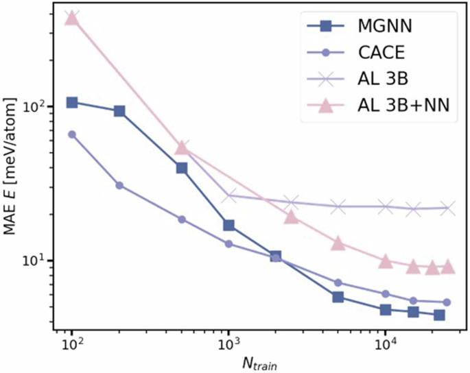
Both alchemical learning (AL) models are from ref. 46, CACE is from ref. 39.
3BPA
The 3BPA dataset was introduced in ref. 45 to evaluate the extrapolation capabilities towards other temperatures using machine-learned interatomic potentials. The training set consists of 500 configurations of the flexible drug-like molecule 3-(benzyloxy)pyridin-2-amine obtained from ab initio molecular dynamics at 300 K, while the test set includes a series of molecular dynamics simulations at 300 K, 600 K, and 1200 K. The root mean squared errors (RMSE) of energy and forces from MGNN for these tests are presented in Table 5, along with results from other state-of-the-art models. ACE(g)53 performs exceptionally well, achieving a significantly superior performance compared to other models. Models like MACE63, NequIP11, BOTNet62, and Allegro12 yield similar results. CACE and MGNN exhibit comparable performance, with MGNN outperforming CACE at 300 K and 600 K, but underperforming at 1200 K. We attribute MGNN’s poorer performance at 1200 K to small training data size (e.g., Fig. 3).
Computational cost
In Table 6, we select models from the Matbench-discovery library66 (e.g., Equiformer v237, GemNet-T29, PaiNN26, SchNet28, SCN67) for comparison with our MGNN. The “F” following MGNN represents the number of scalar features, and “L” represents the number of layers. We compare training times and inference times using the HEA25 dataset. With the exception of MGNN, these models use the default parameters from the Matbench-discovery library66. We select the first 1000 data points from HEA25 without any shuffling for training and inferencing for speed test. The chosen batch size is 2 to ensure all selected models could run smoothly on our NVIDIA GeForce RTX 3090 (24 GB) without errors.
As shown in Table 6, for models with the similar number of parameters, MGNN training and inference speeds are slightly slower than those of GemNet. This is due to the additional processing on angle information for preparing moments, and parameter-learning during the triplet information propagation, both of which slightly reduce computational efficiency. However, MGNN clearly outperforms Equiformer v2 in terms of speed on the same device. This is likely because Equiformer v2 requires the calculation of spherical harmonics by Clebsch-Gordan coefficients, which involves a larger computational load. MGNN’s tensor computations are only performed in the first layer to produce contracted scalars, leading to higher computational efficiency.
Applications
We demonstrate MGNN’s advantage as molecular potential for predicting molecular dynamics simulations of amorphous electrolytes, and rapid simulation of molecular spectra in vacuum conditions for organic molecules. We refer the reader to the Supporting Information S3 for further training, data set, experimental details, and molecular dynamics simulation settings.
Li-ion diffusion in a phosphate electrolyte
Our investigation into the MGNN’s capabilities extends to the kinetic properties of Li-ion diffusion in Li3PO4 solid electrolyte, a material whose conductivity is intricately linked to its crystallinity. The Li3PO4 structure consists of 192 atoms. The simulations are conducted using a time step of 2 fs in the NVT ensemble, employing Nosé-Hoover thermostat68. The dataset includes a 50 ps ab-initio molecular dynamic (AIMD) simulation in the molten liquid state as T = 3000 K, followed by a 50 ps AIMD simulation in the quenched state at T = 600 K. These trajectories are combined, and both the training set of 10,000 structures and the validation set of 1000 are randomly sampled from the combined dataset of 50,000 structures.
Note that the reference results for Allegro in Table 7 are sourced from their paper12. The Ag model is trained and validated using 1000 structures, consist with ref. 12, resulting in a final training performance with energy mean absolute error (MAE) of 0.168 meV atom−1 and force component MAE of 9.5 meV Å−1 on a test set comprising 159 structures. For both the Li3PO4 and Ag datasets, we have achieved competitive results comparable to Allegro.
When evaluating the Li3PO4 test set for the quenched amorphous state, which the simulation is conducted on, we obtained a MAE in the energies of 0.2 meV atom−1, along with a MAE in the force components of 22.92 meV Å−1. Subsequently, we conduct a series of ten MD simulations starting from the initial structure of the quenched AIMD simulation, each lasting 50 ps at T = 600 K in the quenched state, to scrutinize how well MGNN captures the structure and kinetics compares to AIMD. To assess the quality of the structure after the phase change, we compare the all-atom radial distribution functions (RDF) and the angular distribution functions (ADF) of the tetrahedral angle O-P-O (P central atom). As depicted in Fig. 4a, b, MGNN adeptly reproduces both distribution functions. Concerning ion transport kinetics, we evaluate how accurately MGNN models the Li mean-square-displacement (MSD) in the quenched state. Once more, we observe excellent agreement with AIMD, as shown in Fig. 4c. The structure of Li3PO4 is depicted in Fig. 4d. Reference data for the Li3PO4 is obtained from ref. 12.
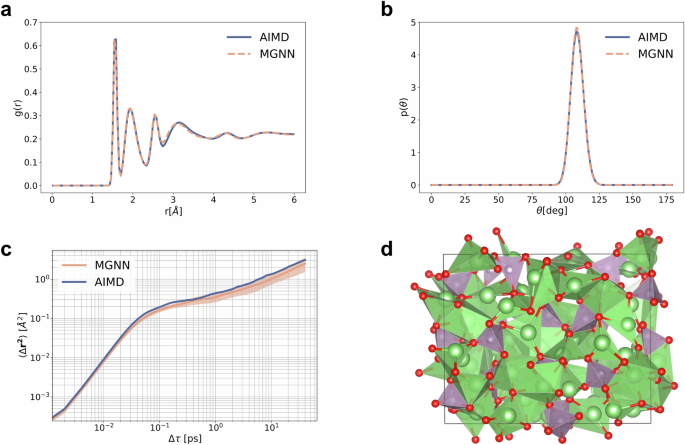
a Radial distribution function. b Angular distribution function of tetrahedral bond angle. All defined probability density functions. c Comparison of the Li MSD of AIMD vs. MGNN. Results are averaged over 10 runs of MGNN, shading indicates ±one standard deviation. d The quenched Li3PO4 structure at T = 600 K. The VESTA77 software was used to generate this figure.
Molecular dynamics simulations are executed in LAMMPS69 using the MGNN pair style, implemented in the SchNetPack 2.055 interface. Other details refer to Supporting Information S3.4. The RDF and ADF for Li3PO4 are computed with a maximum distance of 6 Å (RDF) and 2.5 Å (ADF). The simulation commences from the initial frame of the AIMD quenched simulation. RDF and ADF for MGNN are averaged over ten runs with different initial velocities, with the first 10 ps of the 50 ps simulation discarded in the RDF/ADF analysis to ensure equilibration is adequately accounted for.
Molecular spectra
MGNN is also employed to efficiently compute the infrared and Raman spectra of ethanol. Traditional methods, which might rely on the harmonic oscillator approximation from a singular molecular structure, often neglect critical phenomena such as the diversity of molecular conformations. To secure spectra of superior quality, it is imperative to undertake molecular dynamics simulations, which demand the prediction of forces at each timestep and the calculation of dipole moments and polarizabilities throughout the trajectory. The acquisition of infrared and Raman spectra through the Fourier transformation of time autocorrelation functions of dipole moments and polarizabilities respectively alleviates the complexity and computational intensity of using electronic structure methods. Given the necessity to account for nuclear quantum effects (NQE) for high-fidelity spectra, ring-polymer molecular dynamics (RPMD) simulations are employed, managing multiple replicas of the molecule simultaneously, thereby significantly increasing the computational burden26.
A joint model has been trained on a dataset comprising 8000 conformations of ethanol, supplemented by an additional 1000 molecules each for validation and testing purposes. This model is tasked with the prediction of energies, forces, dipole moments, and polarizability tensors. Dipole moments and polarizability tensors are determined as described in Eqs. (17), (20), respectively. The unified model demonstrates precise predictions for energy, forces, dipole moments, and polarizabilities, as demonstrated in Table 8. Reference data for the ethanol molecule is sourced from ref. 27, and the experimental spectra recorded in the gas phase are obtained from refs. 70,71.
Results from Table 8 reveal that MGNN can acquire expressive atomic tensor embeddings, enabling simultaneous prediction of multiple molecular properties. Particularly noteworthy is MGNN’s superior performance, with energy and force errors approximately a factor of two and three smaller, respectively, compared to FieldSchNet27 and PaiNN26. Additionally, MGNN achieves smaller MAE in force component prediction compared to the equivariant neural network TensorNet38, while attaining results comparable to TensorNet for dipole moments and polarizabilities.
The MGNN potential is then used for classical MD and RPMD72. While both methods can calculate the spectra, they focus on different aspects. The peak positions and intensities of the ethanol infrared spectra (Fig. 5a) computed using classical MD and MGNN closely align with the static electronic structure reference, particularly evident in the C-H and O-H stretching regions at 3000 cm−¹ and 3900 cm−¹. This indicates MGNN’s faithful reproduction of the original electronic structure method. However, in comparison to experimental data, both spectra exhibit shifts towards higher frequencies. In contrast, the MGNN RPMD spectrum demonstrates excellent agreement with experimental results, highlighting the significance of NQEs. Similar trends are observed for the ethanol Raman spectrum (Fig. 5b), where the MGNN RPMD spectrum once again provides the most faithful reproduction of experimental observations.
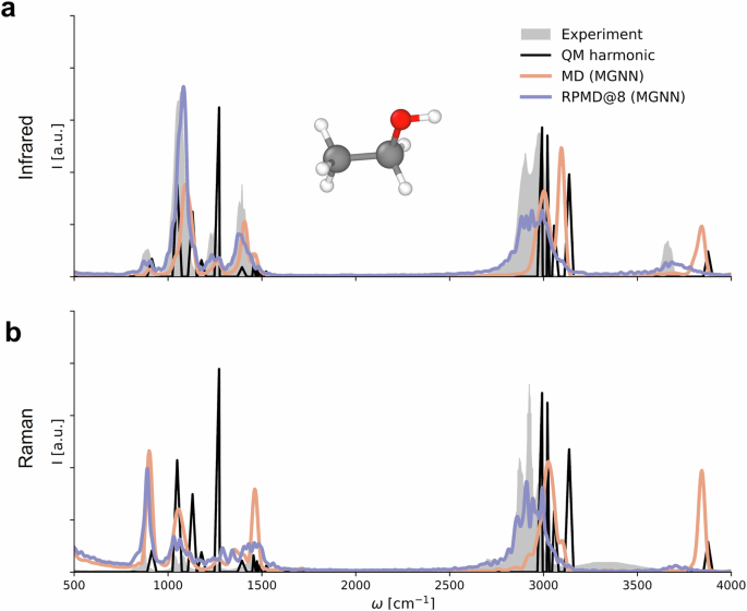
a Infrared spectra of ethanol. b Raman spectra of ethanol. Spectra calculated with the reference method using the harmonic oscillator approximations are shown in black (QM harmonic). Experimental results are shown in gray.
More simulation details are shown in Supporting Information S3.6.
Discussion
In this work, we have introduced MGNN, a Graph Neural Network framework specifically designed for the rapid and accurate prediction of molecular properties. MGNN achieves multiple state-of-the-art results on the QM9 dataset and demonstrates comparable errors to the most recent state-of-the-art models on the revised MD17 dataset. On small molecule MD17-ethanol dataset for stability tests, MGNN shows lower energy errors, lower force errors, and highest stability value. On the 3BPA dataset, the generalization performance of MGNN is validated. On the HEA25 dataset, the learning and computational efficiency of MGNN is demonstrated. Finally, MGNN delivers remarkable consistency with ab-initio calculations, particularly in modeling the migration of lithium ions in electrolytes and in the calculation of infrared and Raman spectra of ethanol.
MGNN’s output module is adept at interfacing with both vector and tensor modules, which enables the model to tailor its output representation to the property being predicted. While our approach does not incorporate vector computations within the molecular representation learning process, the inclusion of these computations in the final output module significantly enhances the model’s computational efficiency. This is exemplified in our application of MGNN to predict vector and tensor features of molecules, such as the dipole moment and polarizability, which are crucial for computing the infrared and Raman spectra of molecules like ethanol in vacuum conditions.
Looking ahead, the potential applications of MGNN are vast and varied, extending to areas such as molecular generation and wavefunction prediction. The rapid and accurate prediction of molecular properties is contingent upon highly precise reference methods, which often come with a high computational cost. As such, machine learning models like MGNN stand to play a pivotal role in surmounting these challenges, thereby driving forward the frontier of computational chemistry and materials science research.
Methods
QM9
The QM9 data set42 consists of 130,831 optimized structures of molecules that contain up to 9 heavy elements from C, N, O and F. On top of the structures, several quantum-chemical properties computed at the DFT B3LYP/6-31 G(2df,p) level of theory are provided.
We use the MGNN model with a cutoff of 5 Å, F = 512, (beta) = 8, and 3 layers. More training details are provided in Supporting Information S3.2.
Revised MD17
The rMD17 data set43 contains 100,000 recomputed structures of 10 molecules from MD1744,60,61, a data set of small organic molecules obtained by running molecular dynamics simulations. The DFT PBE/def2-SVP level of theory, a very dense DFT integration grid and a very tight SCF convergence were used for the recomputations.
We use the MGNN model with a cutoff of 4.5 Å, F = 512, (beta) = 8, and 2 layers. More training details are provided in Supporting Information S3.3.
Li3PO4
The Li3PO4 structure consists of 192 atoms. The Li3PO4 dataset utilized in this study comprises two segments: a 50 ps ab-initio molecular dynamic (AIMD) simulation in the molten liquid state as T = 3000 K, followed by a 50 ps AIMD simulation in the quenched state at T = 600 K. For further details, please refer to ref. 12.
We use the MGNN model with a cutoff of 4 Å, F = 64, (beta) = 8, and 3 layers. More training and simulation details are provided in Supporting Information S3.4.
Ag
Ag system is created from a bulk face-centered-cubic structure with a vacancy, encompassing 71 atoms. For further details, please refer to ref. 12.
We use the MGNN model with a cutoff of 4.5 Å, F = 128, (beta) = 8, and 3 layers. More training details are provided in Supporting Information S3.5.
Molecular spectra
Reference data for the ethanol molecule is sourced from ref. 27, and the experimental spectra recorded in the gas phase are obtained from refs. 70,71. The reference data for ethanol is generated by selecting 10,000 random configurations from the MD17 database44, and re-evaluating them at the PBE0/def3-TZVP60,73 level of theory using the ORCA quantum chemistry package74. SCF convergence is set to tight, and integration grid levels of 4 and 5 are employed during SCF iterations and the final computation of properties, respectively. Computations are expedited using the RIJK approximation75.
We use the MGNN model with a cutoff of 4.5 Å, F = 512, (beta) = 8, and 2 layers. More training and simulation details are provided in Supporting Information S3.6.
MD17-ethanol
MD17 is a collection of eight molecular dynamics simulations for small organic molecules. These data sets were introduced by ref. 44 for prediction of energy-conserving force fields using GDML. Each of these consists of a trajectory of a single molecule covering a large variety of conformations. To demonstrate the stability of MGNN on small organic molecules, we fit to ethanol structures from the MD17 database.
We use the MGNN model with a cutoff of 4.5 Å, F = 512, (beta) = 8, and 2 layers. More training and simulation details are provided in Supporting Information S3.7.
25-element high-entropy alloys
The HEA dataset from ref. 46 consists of 25,630 distorted crystalline structures containing 36 or 48 atoms on bcc or fcc lattices. All the reference energies and forces are computed using density-functional theory (DFT), with the PBESol exchange-correlation functional76.
We use the MGNN model with a cutoff of 6 Å, F = 128, (beta) = 8, and 3 layers. More training details are provided in Supporting Information S3.8.
3BPA
The 3BPA dataset consists of 500 training structures at T = 300 K, and test data at 300 K, 600 K, and 1200 K, of dataset size of 1669, 2138, and 2139 structures, respectively. The data were computed using Density Functioal Theory with the ωB97X exchange-correlation functional and the 6-31 G(d) basis set. For details, we refer the reader to ref. 45.
We use the MGNN model with a cutoff of 4.5 Å, F = 512, (beta) = 8, and 2 layers. More training details are provided in Supporting Information S3.9.

Responses