Efficient GPU-computing simulation platform JAX-CPFEM for differentiable crystal plasticity finite element method

Introducion
In recent years, smart manufacturing has gained significant attention due to its increasing promise in precise and intelligent control of manufacturing processes, enhancing the possibility of forming various materials with diverse combinations of strength and formability1,2,3. The Integrated Computational Materials Engineering (ICME) approach, which has been pivotal in linking the microstructures of materials and manufacturing processes to the resulting properties, has contributed significantly to the forward design process4,5,6,7,8,9,10. Given the rich knowledge in linking material microstructure deformation mechanisms to resulting mechanical properties, Crystal Plasticity (CP) has been developed as a key tool incorporated into ICME11,12,13,14,15,16,17,18,19,20, which predicts the mechanical response of polycrystals up to an industrially relevant component scale21. CP leverages extensive knowledge of single-crystal deformation and dislocations from experimental and theoretical studies, forming the basis for modeling the co-deformation of multiple constituents in a polycrystalline aggregate22,23. Based on Peirce’s work in 198224, the Finite Element Method (FEM) has been widely used to solve CP problems. FEM provides the flexibility in applying complex boundary conditions to arbitrarily shaped geometries. Beyond capturing the homogenized behavior of the sample, the FEM solver is also useful for working on a regular grid of material points, that is, component-scale simulations. These features have made CPFEM crucial in establishing microstructure-processing-property relationships in various study areas, such as texture evolution25,26,27,28, multiphase mechanics29,30,31, crack propagation32,33,34, and so on.
For smart manufacturing, inverse approaches to enable the effective and efficient design of materials microstructure and/or processing parameters are more desirable35,36,37. Inverse design uses target properties as input to derive the initial blank geometry, initial microstructure, and subsequent manufacturing process parameters6. Currently, optimization strategies for inverse design fall into two categories: gradient-free and gradient-based approaches. Gradient-free methods, like genetic algorithm38,39 and Bayesian optimization40,41,42, are used for rational searches in the design parameter space. In contrast, gradient-based optimization, which uses search directions defined by the gradient of the function at the current point, is often advantageous for high-dimensional design problems. For example, for processing design in additive manufacturing, gradient-based optimization is more promising because it needs to handle a high-dimensional design space, including the overall thermal history and heat treatment time for each material point43,44. Despite its potential, the application of gradient-based optimization algorithms based on CPFEM remains largely unexplored for three main reasons. First, integrating case-specific constitutive laws of CPFEM for slip/twinning hardening into the FEM framework can be a lengthy process and has hindered its wider adoption in design and manufacturing. Second, gradient-based algorithms for inverse design require computing the sensitivity, i.e., the gradient of the objective function with respect to target design parameters, which is usually not available by CPFEM codes. Finally, inverse design usually requires solving forward problems in iterations, but CPFEM simulations are computationally extremely expensive. To address these challenges, we have developed JAX-CPFEM based on our recent open-source finite element method library, JAX-FEM45. JAX-CPFEM is an efficient, flexible, and collaborative platform for general-purpose differential CPFEM simulation packages. The following sections will review the current CPFEM software and provide the background and motivation for our developed software.
First, traditional CPFEM approaches often employ a class of constitutive laws for deformation mechanisms as user subroutines, such as UMAT/VUMAT in Abaqus24, incorporated into FEM codes. Implicit schemes in CP typically use a predictor-corrector method to update stresses and solution-dependent state variables at the end of the increment, forming a clockwise loop of calculations during stress determination23, as detailed in Section “Methods”. Subsequently, stress predictions at each integration point of an element are iteratively updated using a Newton-Raphson scheme until convergence. However, deriving the algorithmic tangent modulus, necessary for calculating the Jacobian matrix in Newton’s iterations, is complex and numerically intensive. The inherent non-linearity in the flow rule model that characterizes the crystal deformation system would require considering CP slip/twinning derivatives and Jacobian contributions from each constitutive model46, leading to two main issues. First, it is often simplified by neglecting the derivative of increment of normal vectors to slip planes and slip directions with respect to the strain increments, whose error is on the order of the elastic strain increments47. Second, when incorporating various shear mechanisms and constitutive relationships, deriving case-by-case Jacobian leads to time-consuming analytical considerations15,21. JAX-CPFEM addresses these challenges by utilizing automatic differentiation (AD) in JAX-FEM, which can compute precise derivatives (up to machine precision) of a given function, automatically yielding the Jacobian matrix without manual derivative calculations48. Although the use of AD in the forward problem for finite deformation plasticity has been explored in the last few years49,50,51,52, to the authors’ knowledge, few researchers applied AD in CPFEM. Again, AD simplifies the use of complex mechanical models by automating tangent matrix computations necessary for nonlinear solutions. Also, with a Python frontend, JAX-CPFEM offers a user-friendly experience for users and developers, enabling the efficient handling of large-scale complex problems.
Second, accurate and efficient sensitivity computation (gradient of the objective function to design parameters), essential for gradient-based optimization algorithms, is a critical aspect of solving inverse problems43,53. For example, to understand the effect of each material parameter, a quantitative sensitivity analysis is needed, that is, the derivative of the objective function of stress/strain status of materials to target materials parameters54,55. However, for CPFEM, involving complex constitutive and internal variable details of the process history and environmental factors into the structure–property relations leads to strong nonlinearity of the system. Because of this complicated nonlinearity, the derivation of the sensitivity would require considerable effort. Although JAX-FEM provides automatic sensitivity analysis functions, the current version has incorporated only simple nonlinear models, e.g., hyperelasticity56. For CPFEM, the relationship between strain and stress is implicitly related, so customized differentiation rules will be introduced in JAX-CPFEM. Additionally, the implementation of AD for JAX-CPFEM is superior to non-AD approaches, like the finite-difference-based numerical derivatives, in terms of accuracy while maintaining efficiency especially for high-dimensional material parameter spaces.
Finally, CPFEM simulations are computationally intensive due to the iterative Newton method over residual functions and Jacobian calculations based on complicated constitutive laws. Coupling CPFEM with inverse design for processing/microstructure design requires calling forward problems iteratively, hence, further increasing computational demands57,58,59. Some existing CPFEM software, such as MOOSE60 and PRISMS-Plasticity61, have developed parallel codes that scale well with increasing processing power (CPU cores). However, large-scale numerical calculations are inevitable and still take days (wall time) for practical applications using 32 or 64 processors, while CPU supercomputers with more than 100 processors are not available for most researchers. There is a need for a faster simulation tool to reduce computational time, and the rapid development of Graphical Processing Units (GPUs) offers a potential solution. Specifically, general-purpose GPUs, which specialize in compute-intensive, highly parallel computation, are more capable than CPUs in data processing62. JAX-CPFEM, leveraging the XLA (Accelerated Linear Algebra) backend of JAX48, demonstrates highly competitive performance, especially when GPUs are utilized. Thus, JAX-CPFEM could significantly enhance computational efficiency and promote broader applications in various fields.
In summary, built on the solid foundation of conventional CPFEM, the activation of deformation mechanisms in JAX-CPFEM is related to the physics of the material behavior through the constitutive law, e.g., empirical visco-plastic models63, phenomenological modes64,65, and physics-based models66. In this study, all CPFEM models mentioned later focus on phenomenological constitutive equations and consider dislocation slip as the only deformation mechanism67. We want to emphasize the following three features that differential JAX-CPFEM differ from other CPFEM software:
-
1.
Automatic Constitutive Laws: Free to realize different deformation mechanics represented by constitutive materials laws by evaluating the case-by-case Jacobian matrix using automatic differentiation.
-
2.
Automatic Sensitivity: Differential simulation for sensitivity analysis with respect to design parameters used in single crystal or polycrystal, which can be seamlessly integrated with inverse design.
-
3.
GPU-acceleration: Efficient solution to forward CPFEM (involving complicated nonlinear relations) with GPU acceleration based on array programming style and matrix formulation.
The remainder of the paper is organized as follows. Section “Results” tests three representative forward CPFEM cases, including single-crystal tantalum (body-centered cubic structure), single-crystal copper (face-centered cubic structure), and polycrystal 304 steel (face-centered cubic structure) under various boundary conditions. The computational performance of JAX-CPFEM is further compared with that of a popular CPFEM software, the open-source software MOOSE60. Additionally, this section conducts the sensitivity analysis realized by differential programming and compares the computational cost of the AD technique and finite-difference-based numerical method. Based on the verified sensitivities, we further proposed a pipeline for inverse design and illustrate its power by taking the example of an inverse design of the initial microstructure of a polycrystal metal featuring the targeted mechanical property after applied deformations. Section “Methods” reviews the formulations of CPFEM, including the governing equation, constitutive laws, and numerical implementation, and introduces several key features of JAX-CPFEM that are distinguished from the classic implementation of CPFEM, including automatic constitutive law, array programming style, matrix formulation, and automatic sensitivity. The scheme of notation and other technical information is compiled in Supplementary Note 1.
Results
For benchmarking the performance of JAX-CPFEM, we first tested three numerical examples using Kalidindi’s phenomenological constitutive law65, which considers various crystal structures and boundary conditions. Each case was solved with various levels of mesh resolution using JAX-CPFEM with both CPU-only mode and GPU mode, and MOOSE with MPI for parallel programming. To showcase the inherent efficiency of JAX-CPFEM, leveraging advanced features of JAX, we compare computational performance of JAX-CPFEM on CPU (1 core) with MOOSE using MPI (8 cores). Then in section “AD-based Sensitivity Analysis”, to demonstrate the differentiable capabilities of JAX-CPFEM, we introduced and verified a sensitivity analysis concerning the grain orientation of each grain in the CPFEM simulation, realized through automatic differentiation (AD). Finally, in section “Inverse Design of Grain Orientations via AD-based Sensitivities”, based on the verified AD sensitivities, we conducted the inverse design of grain orientations of each grain in a polycrystal featuring targeted mechanical properties using gradient-based optimization.
Case Study 1: single crystal tantalum (BCC)
We simulated a classic single-crystal tantalum with BCC crystal structure under compressive loading, as shown in Fig. 1a. The domain dimensions are 0.1 mm × 0.1 mm × 0.1 mm, with a strain rate of 0.001 s−1 and quasi-static compressive strain from 0 to −1.25% applied in 50 steps along the x-axis on the right surface. All the other five faces are subject to corresponding constraints. The materials parameters used for Kalidindi’s self and latent hardening law were sourced from recent literature about calibration40, including latent hardening coefficient, saturated slip system strength, hardening constants, and so on. These parameters are summarized in Supplementary Note 2. We first mapped the microstructure of Case 1 to the mesh (163), as mentioned in Fig. 1b, and computed the volume-averaged von Mises stress versus applied strain from both JAX-CPFEM (GPU mode) and MOOSE running with eight processes of MPI parallel programming. Both JAX-CPFEM and MOOSE employed the line search method68 to determine a suitable step size for Newton iteration, which is used for the CP constitutive relationship. In Fig. 1b, the points and the solid line represent the results obtained from JAX-CPFEM and MOOSE, respectively. The results matched exactly with each other, validating the accuracy of our software in a single crystal.

In (a), we show the boundary condition: the compressive experiment compresses the right surface with a prescribed displacement condition and applies constraints on the other five faces. b A comparison of simulation results of the same problem between JAX-CPFEM (points) and MOOSE (line).
For performance benchmarking, this case was solved at various levels of mesh resolution (23, 53, 103, 163, 203, and 253 mesh) using different software. Wall time measurements relative to the number of degrees of freedom (DOF) are shown in Fig. 2. JAX-CPFEM running on GPU demonstrated a significant advantage for moderate to larger-size problems. For instance, for a problem with 52,728 DOF (253 mesh), JAX-CPFEM on CPU and GPU took 1908 s and 629 s, respectively, while MOOSE on CPU with MPI (8 cores) took 2812 s. JAX-CPFEM achieved 1.5× (CPU mode) and 4.5× (GPU mode) acceleration compared to MOOSE with MPI. The computing platforms used for those numerical experiments are summarized in Supplementary Note 3.
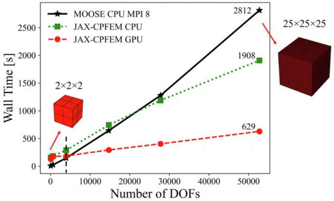
Here, “MOOSE CPU MPI 8” means MOOSE runs with eight processes of MPI parallel programming.
Notably, even without MPI acceleration, JAX-CPFEM on CPU (1 core) outperformed MOOSE with MPI (8 cores) when the problem scales up to 17,783 DOF (203 mesh). The superior performance is due to the XLA compiler infrastructure backend of JAX, which generates optimized code, and the domain-specific tracing just-in-time (JIT) compiler that further allows for high-performance acceleration69. Also, MOOSE’s MPI acceleration is less effective for larger DOF problems due to message passing delay when transient variables exceed the CPU memory limit. Specifically, transient variables, especially from the global stiffness matrix for solving momentum balance, are stored on local storage, leading to delays. Conversely, JAX-CPFEM on GPU exhibits better performance, particularly in more nonlinear cases, as highlighted in the subsequent polycrystal simulation case.
In addition to the computational reasons for the seen speed improvement, another possible reason comes from the numerical aspects. MOOSE uses the Jacobian-Free Newton–Krylov (JFNK) method to solve the nonlinear system of equations of FEM, as detailed in ref. 46. JFNK approximates the effect of the Jacobian through finite differences of the residual vector, which avoids the need to compute and store the Jacobian matrix explicitly and, hence, can handle complex nonlinear problems70. For the CPFEM case study of tantalum mentioned in ref. 46, it was found that JFNK is approximately seven times faster compared to Newton’s method with a numerical Jacobian. Despite these advantages of JFNK used in MOOSE, the method inherently has truncation errors because the Jacobian-vector product is approximated using a first-order difference, which is directly related to the choice of the perturbation parameter. These truncation errors make MOOSE more sensitive to time integration errors, especially at the point of plastic yielding, where the largest error occurs due to the highly nonlinear solution46. Thus, beyond the line search algorithm71 (the same as JAX-CPFEM), MOOSE also employs a sub-increments algorithm72, which allows a smaller time step size to be used at the transition region of plastic yielding to reach convergence. This algorithm enhances solver robustness but increases computational time because it needs more time steps to finish simulations. In contrast, JAX-CPFEM employs AD to get precise Jacobian matrixes (up to machine precision), and thus, it needs fewer time steps at the transition region and further enhances efficiency.
Case Study 2: single crystal copper (FCC)
To further validate JAX-CPFEM for different crystal structures and boundary conditions, we simulated a single-crystal copper with an FCC crystal structure under tensile loading (Fig. 3a). The domain dimensions were 1 mm × 1 mm × 1 mm with a strain rate of 0.1 s−1 and quasi-static incremental loadings from 0 to 0.005 mm applied in 50 steps to the top surface along the z-axis. In this scenario, both the top and bottom surfaces were under-constrained, which had more strict applied constraints. Materials parameters were sourced from the MOOSE benchmark and literature65 (see Supplementary Note 2).
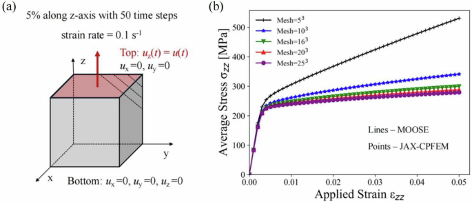
In (a), we show the boundary condition: the tensile experiment fixes the bottom side and pulls the top surface with a prescribed displacement condition. b A comparison of simulation results with different levels of mesh resolution (53, 103, 163, 203, and 253) between MOOSE (lines) and JAX-CPFEM (points).
The plot of the z-z component of volume-averaged stress versus applied strain is shown in Fig. 3b, comparing results from JAX-CPFEM (GPU mode) and MOOSE (CPU MPI), solving the Case 2 with different levels of mesh. Similarly, in Fig. 3b, the points and lines represent the results obtained from JAX-CPFEM and MOOSE, respectively. The mesh-dependent results match perfectly, validating our software’s accuracy in simulating a single crystal under more constraints. This case demonstrated mesh sensitivity compared to the previous case. Although quantitative mesh convergence tests are vital for CPFEM scenarios like this one, they are often overlooked. As Lim et al.73. noted, mesh convergence in the single crystal is influenced by initial crystal orientation, boundary conditions, intragranular heterogeneity, and the hardening model. However, due to computational cost and the need for explicit discretization of individual grains using many finite elements, mesh convergence studies in CPFEM models are more challenging compared to conventional FEM, which is impossible to obtain reasonable estimates of mesh sensitivity in single crystals. Fortunately, GPU-accelerated JAX-CPFEM offers a potential solution for these challenges, since it has the ability to generate enough output results for study, taking a lot of different factors into account while finishing in an acceptable amount of time.
Wall time measurements for different mesh resolutions were also conducted using different software. Figure 4 shows the wall time measurements with respect to the number of DOF, of those last five columns of data points correspond to the problems mentioned in Fig. 3b. JAX-CPFEM on GPU maintained a significant advantage for larger problem sizes. For a problem with 52,728 DOF (253 mesh), it took 6965 s and 1268 s for JAX-CPFEM on CPU and GPU, respectively, compared to 4923 s for MOOSE on CPU with MPI (8 cores). JAX-CPFEM on GPU achieved 1.4× acceleration compared to MOOSE with MPI. Although JAX-CPFEM on CPU/GPU did not scale as well as in Case 1 (4.5×) due to the increased applied constraints, large CPFEM problems can still be readily solved using JAX-CPFEM on GPU. To further demonstrate the computational advantage of JAX-CPFEM, we consider a case study of bi-crystal with two different microstructures (BCC + FCC), as detailed in Supplementary Note 6.
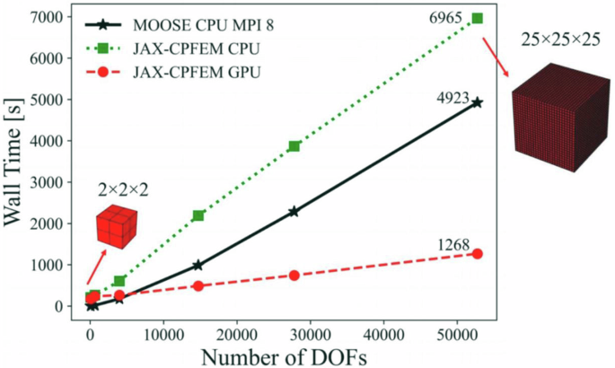
Performance test for Case study 2 with different levels of mesh resolution (23, 53, 103, 163, 203, and 253): single crystal copper (FCC) under a tensile loading boundary condition.
Case Study 3: polycrystal 304 steel (FCC)
CPFEM is a crucial tool in ICME for investigating the structure-property relationship of polycrystals, bridging microscale microstructure and macroscale performance. Based on recent work on 304 steel (FCC)40, we validated JAX-CPFEM software for a general polycrystal simulation. The average equiaxed grain size was set as 8.0 µm, with randomly generated crystallographic texture and crystal orientation due to the lack of experimental data. Using Neper74, an open-source software package for polycrystal generation and meshing, an RVE of 0.016 mm × 0.016 mm × 0.016 mm was constructed, and crystallographic texture was generated using a seed from a random number generator for computing the initial seed position. Crystal orientations for each grain were represented by quaternion rotation and were generated randomly through SciPy75, an open-source package used for statistics, optimization, and so on. In this section, simulations were conducted on a polycrystal case with ensured crystallographic texture and crystal orientations with various mesh resolutions, as shown in Fig. 5a. A quasi-static tensile strain from 0 to 1% with 50 steps was applied along the z-axis at a strain rate of 0.1 s−1, while the bottom surface and a corner were constrained. The plot of the z-z component of volume-averaged stress versus applied strain is shown in Fig. 5b, comparing results from JAX-CPFEM (GPU mode) and MOOSE (CPU MPI), based on the same levels of mesh resolution (163 mesh). Both showed similar results, validating our software for polycrystal simulations.
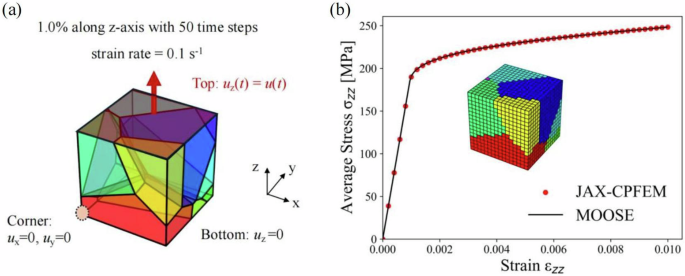
In (a), we show the boundary condition: the tensile experiment fixes the bottom and a corner and pulls the top surface with a prescribed displacement condition. b A comparison of simulation results with the same level of mesh resolution (163) between JAX-CPFEM (points) and MOOSE (line).
Besides homogenized behavior, such as volume-averaged stress, JAX-CPFEM can capture detailed local microstructural information. Utilizing ParaView76, an open-source post-processing software, JAX-CPFEM can generate various visual outputs. For instance, grain distribution and von Moses equivalent stress field can be mapped onto the deformed sample (Fig. 6). A comparison of visualization of the deformed sample between JAX-CPFEM and MOOSE is summarized in Supplementary Note 5, which further validates the accuracy of our software. Such detailed visual outputs can also provide the examination of thresholding, clipping, and slicing of microstructural field for analysis. These visualizations provide additional insights into the local fields within the microstructure, offering a deeper understanding of material behavior and enhancing CPFEM studies.
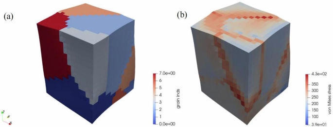
a Grain distribution. b von Mises equivalent stress. The microstructure of the sample is generated using Neper and simulated using conforming FEM discretization scheme with hexahedral elements.
Performance tests with different levels of mesh resolution were conducted, considering 53, 103, 163, 203, and 253 mesh, with wall time measurement comparisons shown in Fig. 7. Compared to the previous single crystal case study, JAX-CPFEM on GPU exhibited a more predominant advantage for polycrystal problems from small to large sizes. For a problem with 52,728 DOF (253 mesh), JAX-CPFEM on CPU and GPU took 6712 s (~1.9 h) and 2203 s (~0.6 h), respectively, compared to 85,892 s (~1 d) for MOOSE on CPU with MPI (8 cores). JAX-CPFEM achieved 12.8× (CPU mode) and 39.0× (GPU mode) acceleration compared to MOOSE with MPI, drastically reducing computation time from days to less than an hour. Polycrystalline simulations in MOOSE with MPI took longer than single-crystal simulations, primarily due to the complexity of polycrystalline materials, including material anisotropy, grain boundary effects, and micromechanical interactions. These factors require more iterative steps for convergence. Each iteration involves solving larger sets of nonlinear equations, increasing computation time. Also, they need to store and manage larger amounts of data related to each grain, such as grain orientations, stress-strain states, etc., increasing memory demands. As mentioned previously, the transient variables exceeding the CPU memory limit are stored in local storage and lead to delays. These factors decrease performance of MOOSE MPI acceleration. JAX-CPFEM on GPU offers a superior alternative; in summary, this degree of acceleration shows great potential to enhance both forward and inverse design in smart manufacturing.
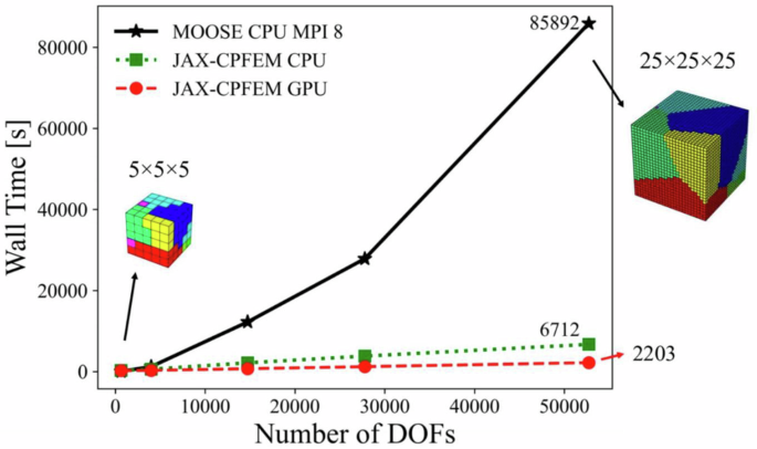
Performance test for Case study 3 with different levels of mesh resolution (53, 103, 163, 203, and 253): polycrystal 304 steel (FCC) under a tensile loading boundary condition.
AD-based sensitivity analysis
Inverse design problems are critical in various engineering applications, such as processing design, microstructure design, and property design. Mathematically, these problems can be formulated as PDE-constrained optimization (PDE-CO) problems77. The key to solving these challenges lies in computing the “sensitivity” (gradient of the objective function to design parameters) accurately and efficiently, which is essential for gradient-based optimization algorithms43. To demonstrate the differentiable capabilities of JAX-CPFEM, we first introduced and verified a sensitivity analysis concerning the grain orientation of each grain in the CPFEM simulation, realized through automatic differentiation (AD). Through these AD sensitivities, we could conduct the inverse design of grain orientations of each grain in a polycrystal featuring targeted mechanical properties using gradient-based optimization, which will be shown in the next section.
In this section, we consider a general copper (FCC) subjected to tensile loadings. The domain dimensions are 0.1 mm × 0.1 mm × 0.1 mm, discretized with 2 × 2 × 2 mesh. Figure 8a shows the boundary conditions and crystallographic geometry. Here, we assume the eight mesh/cells represent different grains of the polycrystal metal, and each with its own crystal orientation represented by three Euler angles (α, β, γ). These angles define a three-dimensional rotation based on sequential rotations around the Z, Y, and X axes relative to its starting position. For the sensitivity analysis of a polycrystal targeting mechanical properties with respect to the grain orientation of each grain, the material response (hat{O}left(theta right)) is defined as the local mechanical status under deformation. Specifically, the average stress σzz is extracted from the corner mesh/cell labeled “1”, located at the bottom-left corner in the x-y plane of the domain, adjacent to the origin (0, 0, 0), as shown in Fig. 8a. The stress status is computed under a 2% applied deformation. The input parameters are summarized and flatten into a vector ({boldsymbol{theta}} =[{theta }_{1},,{theta }_{2},ldots ,{theta }_{24}]), comprising 24 variables, including the three Euler angles (left[{alpha }_{i},,{beta }_{i},{gamma }_{i}right],) applied on all eight mesh/grains. The material response and its corresponding sensitivity are expressed as follows:
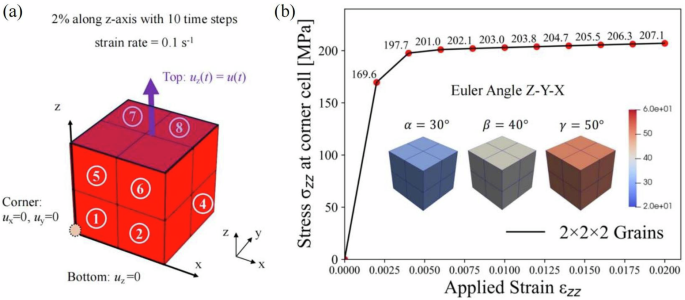
In (a), we show the boundary condition: a polycrystal copper (FCC) with 2 × 2 × 2 mesh/grains under a tensile loading along the z-axis. The tensile experiment fixes the bottom surface and a corner and pulls the top surface with a prescribed displacement condition. b The simulation result of the z-z component of stress σzz extracted from the corner mesh/cell labeled “1” versus applied strain, obtained from JAX-CPFEM. Three Euler angles (left[{alpha }_{i},,{beta }_{i},{gamma }_{i}right]) applied to each mesh/grain are ([30^{circ} ,,40^{circ} ,,50^{circ} ]). The color contour bar in the figure represents the value of Euler angle.
This sensitivity analysis can help us understand the mechanical effect of slight angular deflection of all eight mesh/grains after applying rotation on initial microstructure, additionally, the analysis facilitates automatic inverse design through gradient-based optimization based on experimental mechanical tests. The total derivative of (hat{O}left({boldsymbol{theta }}right)) with respect to parameter variables ({boldsymbol{theta }}) can be calculated through chain rules, see Supplementary Note 4 for details. However, CPFEM involves complicated nonlinear constitutive relations, and the derivation of the sensitivity by deriving analytical expressions through chain rules is quite non-trivial, tedious and error prone. A possible approach is based on numerical differentiation such as finite-difference-based numerical (FDM) derivatives, which is a kind of numerical method for approximating the value of derivatives78. The FDM method is easier to implement. However, it is computationally expensive because it needs to execute the forward CPFEM simulation multiple times, especially when the size of the input parameters is larger than that of the objective function. Furthermore, in situations requiring precise sensitivities, such as in material bifurcation analysis, numerical approximations may introduce significant errors, potentially leading to incorrect conclusions51. In contrast, JAX-CPFEM computes these derivatives at once in a fully automatic manner, which is not only efficient but also feasible for general users.
For comparison, a case study with three Euler angles (left[{alpha }_{i},,{beta }_{i},{gamma }_{i}right]=[30^{circ},,40^{circ},,50^{circ}]) applied to each mesh/grain was used for verification, as shown in Fig. 8b, which also plots the z–z component of average Cauchy stress extracted from the corner cell versus applied strain. The sensitivity calculations for each mesh/cell (No. 1–8) using both AD and FDM-based methods are summarized in Table 1 for sanity check if the derivative is computed correctly. As shown in Table 1, the difference in sensitivity calculations between the two methods is less than 1%, confirming the accuracy of JAX-CPFEM’s differentiability and its ability to utilize AD for precise analytic derivatives even in highly non-linear problems.
While the primary benefit of AD in handling complex non-linear models was often highlighted, the computational cost comparison between AD and non-AD approaches is equally important, yet frequently overlooked. In this CPFEM problem, the number of crystal orientations in each cell typically exceeds that of the objective function, necessitating running forward CPFEM models twice as many times as the number of design parameters. For instance, in the case study in Table 1, 48 forward CPFEM runs (2 × 8 × 3) are required, taking ~4790 s with JAX-CPFEM on GPU. In contrast, AD with differentiable JAX-CPFEM required only 100 s to obtain the sensitivity vector, achieving a 48× acceleration over FDM even on GPU. This efficiency is promising for grain orientation design in CPFEM using gradient-based optimization, which will be elaborated in the next section.
Inverse design of grain orientations via AD-based sensitivities
Microstructure optimization, such as considering the effect of grain size summarized by the traditional Hall-Petch relationship79,80,81, is crucial for overcoming the well-known strength-ductility tradeoff. However, although simulations excel at mapping an input material microstructure to its resulting property, their direct application to inverse design has traditionally been limited by their high computing cost and lack of differentiability35. This section presents a pipeline for inverse design, combining our end-to-end differentiable JAX-CPFEM with gradient-based optimization. We illustrate the power of this approach with an example of the inverse design of initial grain orientations in a polycrystalline metal, aiming to achieve targeted mechanical properties after a specific manufacturing process.
The problem domain is a 0.1 mm × 0.1 mm × 0.1 mm polycrystal copper, discreated with 8 × 8 × 8 hexahedral mesh under the same boundary conditions as shown in Fig. 8a. The objective is to perform an inverse design of the initial crystal orientations of this 512 mesh, each representing different grains. The desired mechanical property is defined by a set of n points representing the local mechanical status (stress-strain curve), extracted from the corner cell adjacent to the origin (0, 0, 0). Let xi and yi represent the n points at different applied strain stages and the stress ({sigma }_{{zz}},) extracted from the corner cell. The input parameters are summarized and flatten into a vector (theta =[{theta }_{1},,{theta }_{2},ldots ,{theta }_{1536}]), including three sequential rotations of Euler angles (α, β, γ) applied on all 512 mesh/grains around the Z, Y, and X axes from the starting position, representing the initial crystal orientation of each grain before deformation. The targeted mechanical properties ({y}_{i},) are the average stresses ({sigma }_{{zz}}) of the corner cell at different applied displacement stages, as shown by the black points in Fig. 9a. In summary, the discretized PDE-CO problem is formulated as
where ({boldsymbol{R}}left({boldsymbol{U}},{boldsymbol{theta}} right){{{:}},{mathbb{R}}}^{N}times {{mathbb{R}}}^{M}to {{mathbb{R}}}^{N}) represents the direct consequence of discretizing the weak form and imposing Dirichlet boundary conditions, and ({boldsymbol{U}}in {{mathbb{R}}}^{N}) is the FEM solution vector of DOF. The objective function ({hat{O}}left({boldsymbol{theta}} right)) is the implicit function that arises from solving the PDE, representing the difference between the targeted and simulated mechanical property:
where ({f}_{{sim},i}(theta )) is the optimized simulation (sim) results at different applied displacement stages obtained from JAX-CPFEM, and (w) is the weight value. It is important to clarify that the sensitivity analysis and subsequent gradient-based optimization are not dependent on the specific choice of the cell as long as the location is consistent in the inverse design pipeline regardless of whether the cell is at the corner or the center cell.
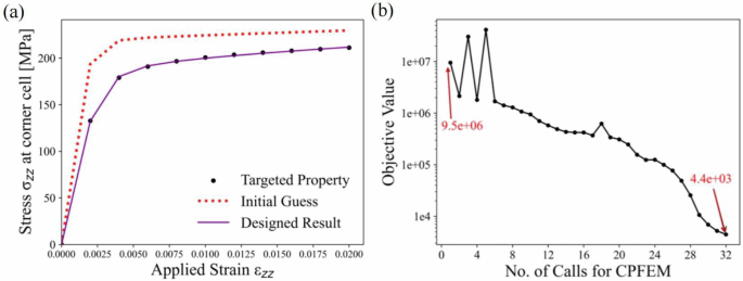
Subfigure (a) shows the targeted local mechanical properties (ground truth) of ({sigma }_{{zz}}) extract from the corner cell under different deformation stage xi, represented by black dots. The red dashed line indicates the JAX-CPFEM simulation outputs based on the initial guess for optimization, which significantly deviates from the targeted properties. The purple line represents JAX-CPFEM simulation results based on the crystal orientations designed by gradient-based optimization. The purple line closely aligns with the targeted properties, demonstrating the robustness of our pipeline. Subfigure (b) illustrates the percentage reduction in the objective function value falls within 0.4% with 32 steps.
The overall workflow for solving inverse design problems uses gradient-based optimization, utilizing search directions defined by the gradient of the function at the current point. The “optimizer” in the algorithm can use any off-the-shelf gradient-based optimization algorithms; for this problem, we used the limited-memory BFGS algorithm82 provided by the SciPy package75 as the optimizer, which is designed for efficiently handling large-scale optimization problems. Based on the chain rule, we can efficiently and automatically compute the tedious and error-prone derivatives (frac{partial hat{O}left({boldsymbol{theta }}right)}{partial {boldsymbol{theta }}}) using the AD function in JAX called “jax.vjp”, which stands for vector-Jacobian product, which has been verified in the above section.
The gradient-based optimization begins with an initial guess with a same rotation for each mesh/grain, meaning the same Euler angles ((alpha =30^{circ},,beta =30^{circ},,gamma =30^{circ})) for each mesh, as shown in the first row of Fig. 10. The corresponding stress ({sigma }_{{zz}}) of the corner cell for this initial guess is shown as the red dashed line in Fig. 9a, which is far from the targeted mechanical properties represented by black dots. Figure 9b shows the optimization iterations, where the objective value is defined in Eq. (3), and each optimization step corresponds to each time the gradient information is queried by the optimizer. Based on the AD-based derivatives calculated at each optimization step, the percentage reduction in the objective function value falls below 1% with only 26 steps, while is about 0.4% when the optimization is completed after 32 steps. Using the designed parameters obtained after 32 gradient-based iterations, we ran JAX-CPFEM to perform a sanity test, ensuring the inverse workflow was processed correctly. The stress-strain curve obtained based on designed parameters, represented by the purple line in Fig. 9a, closely matches the targeted mechanical properties, verifying our inverse design pipeline based on our differentiable JAX-CPFEM. The designed parameters, Euler angles (left[{alpha }_{i},,{beta }_{i},{gamma }_{i}right]) for the 512 mesh/grains, are shown in the second row in Fig. 10. The corresponding inverse pole figures depicting the designed crystallographic orientation of grains are shown in the third row, while the initial guess of crystallographic orientation of grains is labeled by black boxes. This information can provide insights for future microstructure design via smart manufacturing.
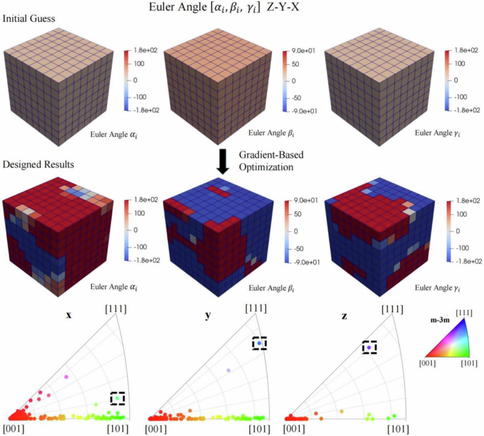
The first row shows the initial guess for the gradient-based optimization, where each mesh is assigned the same Euler angles ((alpha =30^{circ},,beta =30^{circ},,gamma =30^{circ})). The second row displays the Euler angles designed for each cell after 32 iterations of gradient-based optimization. Inverse pole figures depicting the designed crystallographic orientation of grains for targeted properties, corresponding to a specific direction in the reference frame of crystal, are shown in the third row. The crystallographic orientations of initial guess are also identified on inverse pole figures by black dashed boxes.
In summary, this section proposed an inverse design of crystal orientations in polycrystalline materials as an example, demonstrating the robustness and efficiency of our pipeline, which integrates differentiable JAX-CPFEM with a general optimizer. We highlight three key contributions of our pipeline that distinguish it from others:
-
1.
Scalability to high-dimensional inverse problems: Leveraging gradient-based optimization supported by the differentiable JAX-CPFEM, our pipeline effectively addresses high-dimensional inverse problems. For instance, in this section, the input variables’ dimension is 1536, whose complexity is challenging for other gradient-free optimization methods like Bayesian approaches.
-
2.
Handling ill-posed problems: While the example presented in this section is an ill-posed problem with non-unique and multiple solutions, our pipeline has the potential to incorporate various regularization techniques to stabilize and make the problem well-posed. These techniques include Tikhonov regularization83, adding constraints, and smoothing84, which are areas we intend to explore further in future research.
-
3.
Versatility beyond crystal orientation design: Beyond crystal orientation designs, our gradient-based inverse design pipeline is adaptable to various manufacturing applications, including the design of initial material microstructures and the subsequent manufacturing process parameters. Also, efficient solution to forward CPFEM (involving complicated nonlinear relations) with GPU acceleration makes a wide range of applications of the inverse design pipeline possible.
Discussions
In the “Results” section, we presented JAX-CPFEM, an open-source, GPU-accelerated, and differentiable 3-D crystal plasticity finite element method (CPFEM) software package. Compared with existing codes of CPFEM, JAX-CPFEM is featured with its affordability, flexibility, and multi-purpose, making it accessible to a wider range of users. Specifically, JAX-CPFEM is fully vectorized and uses automatic differentiation (AD) to computationally evaluate the Jacobian matrix, ensuring constitutive laws and momentum balance can be solved within the Newton scheme. This flexibility allows general users to handle complex, non-linear constitutive materials laws without manually deriving the Jacobian matrix, for example, coupling different deformation mechanics and internal variables. We validated JAX-CPFEM across three CPFEM problems with different crystal structures and boundary conditions, by comparing it with the existing software MOOSE. Currently, JAX-CPFEM supports phenomenological CPFEM models, including Kalidindi’s and Peirce’s hardening laws. Work on integrating physics-based constitutive models is ongoing.
Furthermore, we compared the performance of JAX-CPFEM (in both CPU-only and GPU modes) with MOOSE using MPI across various scenarios. Leveraging AD, array programming, and matrix formulation, JAX-CPFEM demonstrated significant computational efficiency, particularly with GPU acceleration. For larger-size single crystal problems, JAX-CPFEM (GPU mode) achieved about 1.4–4.5× speedup compared to MOOSE with MPI (8 cores). For larger-size polycrystal problems, JAX-CPFEM (GPU mode) achieved about 39× acceleration compared to MOOSE with MPI (8 cores), reducing computation time from days to under an hour. This greater acceleration in polycrystal simulations is due to the added complexity of polycrystalline materials, including anisotropy, grain boundary effects, and micromechanical interactions, which require more iterative steps and larger data management. For MOOSE, MPI’s need for frequent synchronization and communication between cores slows down its performance, especially when managing large-scale data85. In contrast, GPUs efficiently handle these challenges with their parallel processing power, higher memory bandwidth, and optimization for matrix operations86, making JAX-CPFEM on GPU has a clear speedup in solving polycrystalline problems. Currently, the largest problem solvable with a single 48 GB memory NVIDIA GPU is around 5 million DOF, we plan to leverage the capabilities of JAX for distributed computing to extend support for multi-GPU setups. These enhancements are part of our ongoing effort to make JAX-CPFEM more scalable for larger-scale problems.
Additionally, sensitivity analysis of a polycrystal copper targeting mechanical properties with respect to the initial crystal orientations of each grain used in CPFEM simulations demonstrated the differentiable capability of JAX-CPFEM for end-to-end sensitivity calculation. In the case of considering 8 mesh/cells, AD achieved a 48× acceleration over the FDM-based numerical method even on GPU, highlighting significant computational efficiencies compared to non-AD approaches. Through the AD-based sensitivity, JAX-CPFEM performed an inverse design of initial grain orientations in a polycrystalline metal featuring targeted mechanical properties, based on a pipeline combining JAX-CPFEM with gradient-based optimization. This inverse case study illustrates the capability of differentiable JAX-CPFEM for seamlessly integrating with inverse design, which could facilitate research in the co-design of material types, initial microstructure and processing parameters. For instance, in directed energy deposition (DED) additive manufacturing (AM), pores are common microstructural features that influence deformation, damage, and failure87,88. What specific mechanical deformation processes after the AM process lead to certain regions having particular pore shapes, sizes, and distributions? Addressing this question can directly enhance the mechanical properties of AM products. To find a solution, by treating the process parameters as the design space, JAX-CPFEM could be used in combination with a gradient-based optimization algorithm to iteratively minimize the difference between predicted and target pore shapes. Additionally, the co-design of material types and initial microstructure through inverse design using JAX-CPFEM may face manufacturing challenges if, for example, the differences in rotation angles between adjacent parts are too large. However, we can further incorporate constraints into this pipeline to make the inverse-designed products more feasible for integration with smart manufacturing.
Methods
This section reviews the formulations of CPFEM, including the governing equation, constitutive laws, and numerical implementation. Then, we introduce several key features of JAX-CPFEM that are distinguished from the classic implementation of CPFEM, including automatic constitutive law, array programming style, matrix formulation, and automatic sensitivity.
Governing equation
The kinematics of isothermal finite deformation describes the process where a body originally in a reference configuration, (Bsubset {R}^{3}), is deformed to the current configuration, (Ssubset {R}^{3}), by a combination of externally applied forces and displacements over a period of time22. In this treatment, we choose the perfect single crystal as the reference state, which has the advantage of a constantly unchanged reference state. The balance of momentum in reference configuration (ignoring inertial term and body force) is expressed as follows:
where ({boldsymbol{P}}) is the first Piola-Kirchhoff stress tensor, ({boldsymbol{u}}) is the displacement field to be solved, ({{boldsymbol{u}}}_{D}) is the boundary displacement, ({boldsymbol{t}}) is the traction and ({boldsymbol{n}}) is the outward normal vector.
Crystal plasticity constitutive model
The deformation gradient ({boldsymbol{F}}) is assumed to be multiplicatively decomposed in its elastic and plastic parts89:
where ({{boldsymbol{F}}}^{{rm{e}}}) is the elastic deformation gradient induced the reversible response of the lattice to external loads and displacements, and ({{boldsymbol{F}}}^{{rm{p}}}) is the plastic deformation gradient, an irreversible permanent deformation that persists when all external forces and displacements that produce the deformation are removed.
The total plastic velocity gradient can be expressed in terms of the plasticity deformation gradient as
The elastic Lagrangian strain ({{boldsymbol{E}}}^{{rm{e}}}) is defined as
The second Piola-Kirchhoff stress ({boldsymbol{S}}) is given by
where ({mathbb{C}}) is the elastic modulus. The Cauchy stress ({boldsymbol{sigma }}) is given by
The first Piola-Kirchhoff stress ({boldsymbol{P}}) is given by
The plastic velocity gradient ({{boldsymbol{L}}}^{{rm{p}}}) is computed as the sum of contributions from all slip systems.
where ({dot{gamma }}^{alpha }) is the slip rate for slip system (alpha), ({{boldsymbol{s}}}_{0}^{alpha }) and ({{boldsymbol{m}}}_{0}^{alpha }) are unit vectors describing the slip direction and the normal to the slip plane of the slip system in the reference configuration. The resolved shear stress ({tau }^{alpha },) is defined as
The slip rate ({dot{gamma }}^{alpha }) is expressed as a power law relationship:
where (dot{{gamma }_{0}}) is a reference slip rate, ({g}^{alpha }) is the slip resistance (or critical resolved shear stress), and (m) is the strain rate sensitivity exponent. The rate of slip resistance (dot{{g}^{alpha }},) is given by
where ({h}^{alpha beta },) is the rate of strain hardening on slip system (alpha) due to a shearing on the slip system (beta). Kalidindi et al. 65 self and latent hardening law gives
Respectively, ({g}_{{rm{ini}}}) is the initial slip resistance and ({g}_{{rm{s}}a{rm{t}}}) is the saturation slip resistance. (a) and ({h}_{0},) are slip hardening parameters which are taken to be identical for all slip systems. ({q}^{alpha beta },) is the matrix describing the latent hardening behavior of a crystallite. Here,
where (r) is the ratio of the latent hardening rate to the self-hardening rate.
Numerical aspects of CPFEM
The quasi-static process is described by Eq. (4). Based on array programming and AD, JAX-FEM can solve such second-order elliptic partial differential equation by Newton’s method (see ref. 45 for details). For this section, we focus on introducing the constitutive model in its continuous form and discretizing the constitutive model in time for implementation in the JAX-FEM solver.
Since ({{boldsymbol{P}}}_{n}) and ({{boldsymbol{F}}}_{n}) are implicitly related in CPFEM, current studies often use a predictor-corrector scheme following the clockwise loop of calculations, as shown in Fig. 11. By this way, one could start predicting any of the quantities involved, follow the circle and compare the resulting quantity with the predicted one. Subsequently, the prediction will be updated using Newton’s scheme.
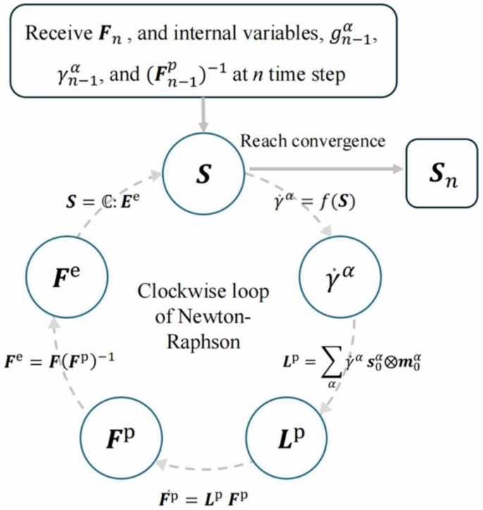
Clockwise loop of calculations during stress determination (({boldsymbol{S}}) second Piola-Kirchhoff stress, ({dot{gamma }}^{alpha }) slip rate, ({{boldsymbol{L}}}^{{rm{p}}},) plastic velocity gradient, ({{boldsymbol{F}}}^{{rm{p}}}) plastic deformation gradient, ({{boldsymbol{F}}}^{{rm{e}}}) elastic deformation gradient).
Following the idea by Roters et al.22 and MOOSE60, we stick to the second Piola-Kirchhoff stress ({boldsymbol{S}}) based formulation. Based on ({{boldsymbol{S}}}_{n}), solving (,{{boldsymbol{P}}}_{n}) is straightforward. At current time step (n), we are given the total deformation gradient ({{boldsymbol{F}}}_{n}) at any integration point and some internal variables from previous time step ((n-1)), including ({g}_{n-1}^{alpha }), ({gamma }_{n-1}^{alpha }), and ({({{boldsymbol{F}}}_{n-1}^{p})}^{-1}), we first solve the following nonlinear equations to get ({S}_{n}):
where ({boldsymbol{R}}_{C}:{{mathbb{R}}}^{dim times dim }times {{mathbb{R}}}^{dim times dim }to {{mathbb{R}}}^{dim times dim }) is the residual function. The residual function in (17) is explicitly expressed as the following:
where ({boldsymbol{F}}_{n}^{e}) is explicitly computed from ({boldsymbol{S}}_{n}) through the clockwise loop shown in Fig. 11. In the following description, we discretize the equations in time and show how to map from ({{boldsymbol{S}}}_{n}) to ({{boldsymbol{F}}}_{n}^{e}).
Step 1: from ({boldsymbol{S}}) to (dot{{{boldsymbol{gamma }}}^{{boldsymbol{alpha }}}}). In this case, we use Kalidindi’s hardening law as an example. Based on Eq. (12),
Discretize both Eqs. (13) and (14) in time as
As mentioned before, ({g}_{n-1}^{alpha }) and ({gamma }_{n-1}^{alpha }) are stored internal variables from previous step.
Step 2: from (dot{{{boldsymbol{gamma }}}^{{boldsymbol{alpha }}}}) to ({{boldsymbol{L}}}^{{bf{p}}}). Based on previous step’s calculation, ({gamma }_{n}^{alpha }-{gamma }_{n-1}^{alpha}) is available, and we discretize Eq. (11) as
Step 3: from ({{boldsymbol{L}}}^{{bf{p}}}) to ({{boldsymbol{F}}}^{{bf{p}}}). We continue to discretize Eq. (6) as
where ({boldsymbol{I}}) is the second order identity tensor and (Delta t) is the time step size. ({left({{boldsymbol{F}}}_{n-1}^{{rm{p}}}right)}^{-1}) is also one of the stored internal variables from the previous step.
Step 4: from ({{boldsymbol{F}}}^{{rm{p}}}) to ({{boldsymbol{F}}}^{{rm{e}}}). Based on Eq. (5), it follows
Up to this point, we are able to evaluate the residual function ({{boldsymbol{R}}}_{C}) in Eq. (18) given ({{boldsymbol{S}}}_{n}). Solving the equation requires Newton’s method:
where the superscript (k) denotes the iteration step in Newton’s method. (frac{partial {boldsymbol{R}}_{C}}{partial {boldsymbol{S}}_{n}^{(k)}}:{{mathbb{R}}}^{dim times dim times dim times dim }) is the Jacobian matrix. Several examples of notations used in the chain rule, including Eq. (25)–(28), are given in Supplementary Note 1. To help the solver to converge, similar to MOOSE, we use the line search method68 to determine a suitable value for the step size (theta).
Automatic constitutive laws
As the common practice in nonlinear finite element methods, Newton’s method is used to solve the governing equation in Eq. (4), as shown in Algorithm 1. At each integration point, the information of the first Piola-Kirchhoff stress tensor ({{boldsymbol{P}}}_{n}) and the tangent tensor (frac{partial {{boldsymbol{P}}}_{n}}{partial {{boldsymbol{F}}}_{n}}) are required. Due to the nonlinear CP constitutive relationship, ({{boldsymbol{P}}}_{n}) is obtained by a quadrature-level Newton’s method based on the ({{boldsymbol{F}}}_{n}) and internal variables, while (frac{partial {{boldsymbol{P}}}_{n}}{partial {{boldsymbol{F}}}_{n}}) is obtained through implicit differentiation.
In practice, ({{boldsymbol{S}}}_{n}) is obtained first, based on which ({{boldsymbol{P}}}_{n}) is calculated (see Eq. (8)–(10)). Given ({{boldsymbol{F}}}_{n}) and the material parameters from the previous time step, the update of ({{boldsymbol{S}}}_{n},) during quadrature-level Newton iterations relies on the Jacobian matrix (frac{partial {{boldsymbol{R}}}_{C}}{partial {{boldsymbol{S}}}_{n}}), as shown in Eq. (25). For traditional treatment, e.g., Kalidindi’s constitutive law, the CP Jacobian matrix must be derived manually, including the contributions from (frac{partial {({{boldsymbol{F}}}_{n}^{{rm{p}}})}^{-1}}{partial {({{boldsymbol{L}}}_{n}^{{rm{p}}})}^{-1}}), (frac{partial {({{boldsymbol{L}}}_{n}^{{rm{p}}})}^{-1}}{partial {dot{gamma }}_{n}^{alpha }}), (frac{partial {dot{gamma }}_{n}^{alpha }}{partial {tau }_{n}^{alpha }}), and (frac{partial {tau }_{n}^{alpha }}{partial {{boldsymbol{S}}}_{n}}):
Algorithm 1
Newton’s Update
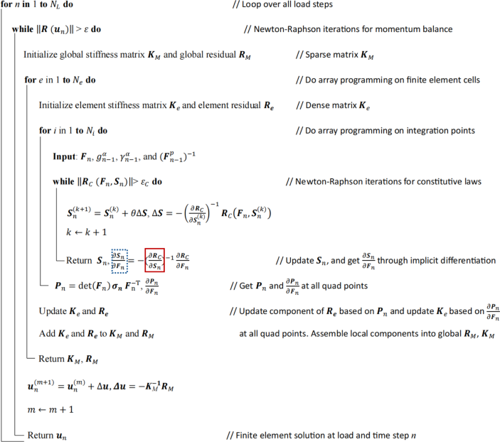
Forming the exact analytical derivatives for each component in Eq. (26) is tedious due to the inherent non-linearity in the flow rule model. The exact CP Jacobian can even be intractable, especially when considering (1) multiple deformation mechanisms, e.g., slip, twinning and their interactions; (2) different constitutive relationships, e.g., Peirce’s self-hardening law24 and so on; (3) applied multi-physics conditions, e.g., heating and so on. Consequently, simplifications are often made, neglecting the derivative of the increment of normal vectors to slip planes and slip directions with respect to strain increments. However, this simplified form introduces errors of the same order as the elastic strain increments47. In contrast, JAX-CPFEM utilizes jax.jacfwd, a core function for AD, to automatically evaluate the Jacobian matrix (frac{partial {{boldsymbol{R}}}_{C}}{partial {{boldsymbol{S}}}_{n}}) mentioned in the red solid-line box, eliminating the need for users to manually consider these factors into CPFEM on a case-by-case basis. It should be noted that AD provided by JAX has its default rule to calculate derivatives of functions with singular points. The AD derivatives of functions written in jax.numpy are the same as those calculated by hand. For Kalidindi’s constitutive law applied in our framework, there are two non-smooth equation, including Eq. (13) with absolute value calculation and Eq. (15) with signum functions. For the “signum” function, both left derivative and right derivative are the same, i.e., 0. For the “absolute” function, JAX takes the left derivative, which is −1 at the singularity point 0.
Similarly, (frac{partial {{boldsymbol{P}}}_{n}}{partial {{boldsymbol{F}}}_{n}}) will be available once (frac{partial {{boldsymbol{S}}}_{n}}{partial {{boldsymbol{F}}}_{n}}) is obtained. In CPFEM, the relationship between ({{boldsymbol{S}}}_{n},) and the strain ({{boldsymbol{F}}}_{n}) is implicit, as shown in the residual function mentioned in Eq. (17), linked by the non-linear constitutive relationship of slip hardening laws shown in Fig. 1. The calculation of (frac{partial {{boldsymbol{S}}}_{n}}{partial {{boldsymbol{F}}}_{n}}) hence falls into the framework of “implicit differentiation”90,91. Although JAX-FEM provides automatic sensitivity analysis functions, it is designed for simpler non-linear models, such as hyperelasticity56, and cannot be directly applied to compute this derivative in CPFEM. To address this “implicit differentiation” problem of (frac{partial {{boldsymbol{S}}}_{n}}{partial {{boldsymbol{F}}}_{n}}) at each integration point of the mesh, we take the total derivative of Eq. (17) with respect to ({{boldsymbol{F}}}_{n}) and obtain
Therefore,
In JAX-CPFEM, we use a function decorator, jax.custom_jvp, to introduce customized differentiation rules. Specifically, we set up a JAX-transformable function to get the value of ({{boldsymbol{S}}}_{n},) based on the results of clockwise loop of calculations, which serves as the forward function. Based on this forward function, we further define customized Jacobian-Vector Product (JVP) rules with (frac{partial {{boldsymbol{R}}}_{C}}{partial {{boldsymbol{S}}}_{n}}) and (frac{partial {{boldsymbol{R}}}_{C}}{partial {{boldsymbol{F}}}_{n}}) in Eq. (28) evaluated using normal AD, jax.jacfwd. This approach allows us to calculate the value of (frac{partial {{boldsymbol{S}}}_{n}}{partial {{boldsymbol{F}}}_{n}}) at each integration point, as shown in blue dotted-line box in Algorithm 1. A detailed introduction to implicit differentiation and its implementation in JAX function can be found in92.
Array programming
Based on automatic linearization, JAX-CPFEM works directly with the weak form and performs the linearization based on AD for each load step. This method enables the assembly of the finite-dimensional linear system discretized by the Galerkin FEM, as shown in Algorithm 1, where Ne is the total number of elements and Ni is the number of integration points associated with each finite element cell. Instead of using for-loops as is common practice in Fortran or C/C++ to go through all elements, JAX-CPFEM employs the array programming style (in the same spirit of NumPy24) for acceleration. This approach is used in solving Newton’s linear problem of momentum balance. Additionally, a key feature in JAX-CPFEM is the use of array programming to map the computation at all integration point for all finite element cells at once. By utilizing jax.vmap, a core function of JAX for vectorized operations, the program can automatically vectorize and efficiently operate over arrays representing batches of inputs, fully utilizing GPU acceleration.
Matrix formulation
For CP, it is essential to update the characteristics of each slip system, including slip resistance, slip rate, and so on, based on the kinetics and interactions of each slip system. Typically, there are more than twelve slip systems22, and traditional software implementations in Fortran or C/C++ use for-loops to perform these computations. To fully utilize GPU acceleration, we transform constitutive laws from equation formulation to matrix formulation. For example, in Kalidindi’s constitutive model, shown in Eq. (21), the update of slip resistance on each slip system is transformed from an equation-based computation to a matrix-based computation:
where ({boldsymbol{g}}{{in }}{{mathbb{R}}}^{{rm{alpha }}times 1}) is the vector of increment of slip resistance on each slip system, ({boldsymbol{Q}}{{in }}{{mathbb{R}}}^{{rm{alpha }}times {rm{alpha }}}) is the matrix of coefficient matrix of interactions between each slip system, and ({boldsymbol{c}}{{in }}{{mathbb{R}}}^{{rm{alpha }}times 1}) is the remaining part on the right-hand side.
Automatic sensitivity
The successful computation of “sensitivity”, i.e., the gradient of the objective function to design parameters, is crucial for understanding the effect of different materials/microstructure/processing parameters on the mechanical properties of either single crystal or polycrystal metals. We formulate the CPFEM forward simulations as follows
where ({boldsymbol{U}}{{in }}{{mathbb{R}}}^{N}) is the FEM solution vector of degrees of freedom (DOF), ({boldsymbol{theta }}{{in }}{{mathbb{R}}}^{M}) is the materials/microstructure/processing parameter vector. ({boldsymbol{R}}left({{cdot}},,{{cdot}}right){{{:}}{mathbb{R}}}^{N}{{times }}{{mathbb{R}}}^{M}{{to }}{{mathbb{R}}}^{N}) is the constraint function, which represents the discretized governing partial difference equation (PDE). To conduct a sensitivity analysis of the parameter variables, we define the materials response as (Oleft({boldsymbol{U}},{boldsymbol{theta }}right){{{:}}{mathbb{R}}}^{N}{{times }}{{mathbb{R}}}^{M}{{to }}{mathbb{R}}), which could be the sum of n points/stages defining simulation results (i.e., strain–stress curve of the polycrystal). A reduced formulation is used to embed the PDE constraint so that the materials response can be re-formulated as
where ({boldsymbol{U}}({boldsymbol{theta}} )) is the implicit function that arises from solving the PDE. The total derivative of (hat{O}left({boldsymbol{theta }}right)) with respect to parameter variables ({boldsymbol{theta }}) can be calculated through chain rules, see Supplementary Note 4 for details. Nevertheless, CPFEM entails complex nonlinear constitutive relations, and obtaining the sensitivity through analytical derivations using the chain rule is highly challenging, labor-intensive, and prone to errors.
A possible approach is based on numerical differentiation such as finite-difference-based numerical derivatives (FDM), which is a kind of numerical method for approximating the value of derivatives. Assuming a small perturbation of the model parameters, the model can be linearized with respect to the perturbation and the new material response as follows
where
({boldsymbol{J}}) is the gradient, namely, the derivatives of material response with respect to the set of parameter variables. To compute the Jacobian matrix, one of the parameters is perturbed by (Delta theta) as follows
and the response of the perturbed model is determined by the FEM analysis of the RVE. This procedure is repeated for each parameter in the model and resulting result is given by,
The FDM is easy to implement. However, it is computationally expensive because it needs to execute the forward CPFEM simulation multiple times, especially when the size of the input parameters is larger than that of the objective function (e.g., (Mgg 1) in this scenario). In addition, when accurate sensitivities are critical, such as in material bifurcation analysis, numerical approximations can lead to substantial errors, which may result in inaccurate conclusions51.
JAX-CPFEM obtains these derivatives at once in a fully automatic manner, which is not only efficient but also feasible for general users. In addition, mathematically, inverse problems like calibration can be formulated as PDE-constrained optimization problems77. The successful computation of “sensitivity” is also the basis for gradient-based optimization algorithms. Namely, JAX-CPFEM also paves the way for gradient-based optimization algorithms to be applied to inverse problems.


Responses