OBI-CMF: Self-supervised learning with contrastive masked frequency modeling for oracle bone inscription recognition

Oracle bone inscriptions (OBI)¹, as a symbolic writing system, are extensively utilized for divination during the Shang Dynasty ~3300 years ago. These characters are typically inscribed on tortoise shells and animal bones for divination². Acting as a medium for documentation, they preserve a wealth of historical information relating to population, agricultural practices, and social customs. The study of OBI is of great significance to experts in various fields, as it provides valuable materials on many aspects of ancient Chinese society. Although significant advancements have been made in deciphering these characters, a substantial number remain undeciphered. Given that oracle bones are vulnerable to damage and direct observation may lead to damage to the originals, OBI Rubbings (OBIR) have become the primary tool for studying OBI. Manual recognition of OBI relies on the experience and knowledge of experts, but it is time-consuming and labor-intensive. With the rapid development of deep learning, scholars have attempted to use convolutional neural networks (CNN)^3,4,5 to improve the efficiency and accuracy in recognizing OBI.

Due to the passage of thousands of years, the tortoise shells and animal bones bearing the script have undergone natural erosion and human-made damage. As depicted in Fig. 1a, the damage leads to generally poor image quality and significant noise, which dramatically poses a considerable challenge to accurate recognition. In addition, stylistic differences between engravers and the evolution of characters over time create significant visual heterogeneity. These factors result in substantial differences in the appearance of the same character across different images. The intra-class variability is shown in Fig. 1b, which significantly increases the complexity of the classification model for accurately recognizing the same character.

a OBIR corrupted by noise. b Different variant forms of the same OBI character.

Full size image

To overcome the above issues, UDCN⁶ employs a domain adaptation method, which enhances the model’s discriminative ability by incorporating consistency regularization and transition loss derived from the transformation matrix of different augmented views. This method effectively mitigates the model’s limitations in dealing with image noise and intra-class differences. However, the training process of UDCN relies on labeled data that is akin to the target dataset, which puts forward specific requirements for the acquisition of labeled data.

As depicted in Fig. 2, the OBI dataset exhibits a significant long-tailed distribution, where a few classes dominate with a large number of samples, while most classes contain only a small number. For instance, in the OBC306 dataset ⁷, the class “zhen (贞)” includes 25,898 samples, while the class “cheng (乘)” is only <10 samples. This imbalance not only increases the difficulty of training classification models but also challenges the ability to extract generalizable and robust features under noisy conditions and substantial intra-class variability. While existing methods, such as OCR-ADA⁸, attempt to alleviate data imbalance through hybrid data augmentation techniques like static Mixup⁹ and dynamic generative adversarial network (GAN)¹⁰, their reliance on supervised learning and annotated data often limits their ability to fully capture the intrinsic characteristics of OBIR. Our research shifts the focus toward improving the capability of feature extraction under imbalanced conditions, aiming to address the challenges of noise and intra-class variability and provide a deeper understanding of the underlying data structure in OBI datasets.

Data distributions of the OBC306 dataset.

Full size image

To address the above challenges, an effective self-supervised OBI recognition method named OBI-CMF is proposed. Our method combines the reconstruction task from the self-supervised learning paradigm with contrastive learning, and it integrates these tasks effectively in both spatial and frequency domains. Given that the direct application of supervised learning to OBI datasets may lead to imbalanced feature learning of majority and minority classes coupled with the limited labeled rubbings, we initially employ self-supervised learning methods to capture the intrinsic features of the OBIR. To mitigate the noise presented in the OBIR, the histogram of oriented gradients (HOG)¹¹ is selected as the target for the reconstruction task. Our approach effectively reduces noise interference and enhances the capability of the model to learn the OBIR features. In addition, we utilize frequency domain masking technology to perform high-pass and low-pass filtering on the OBIR and independently process the filtered images. Subsequently, through contrastive learning, our OBI-CMF can comprehensively learn the global features of the OBIR, thus more accurately recognizing OBI of different styles and historical periods.

Through the above improvements, our OBI-CMF shows excellent performance in processing both balanced and imbalanced OBI datasets while effectively dealing with noise interference and the diversity of Oracle characters, which significantly improved the accuracy of identification and the robustness of the model.

Our contributions can be summarized as follows:

(1) We propose a simple yet effective self-supervised learning method named OBI-CMF to learn robust and discriminative OBIR features. By effectively combining contrastive learning and masked modeling, our approach significantly enhances the model’s performance in OBIR processing.

(2) We innovatively adopt Oracle’s dual-domain feature learning strategy in the spatial and frequency domains. This strategy enables the OBI-CMF to learn more comprehensive and high-quality OBIR features through mutual supervision and promotion between the two domains. This not only improves the model’s resistance to noise but also enhances its ability to recognize changes in the OBI characters.

(3) To the best of our knowledge, this is the first work that utilizes frequency domain knowledge in OBI recognition. We conduct extensive experiments on three variants of the OBC306 dataset and evaluate the performance of the OBI-CMF from both balanced and imbalanced data perspectives. The results demonstrate that our OBI-CMF achieves excellent performance in various contexts and showcases its potential for practical applications.

OBI recognition

OBI carries profound historical significance, so their accurate distinction plays a crucial role in human society. Consequently, Liu et al.¹² apply several classical convolutional neural networks^{13,14,15,16,17} to the analysis of OBI characters, achieving commendable results. For example, Zhang et al.¹⁸ utilize DenseNet¹⁹ to map OBI images into Euclidean space and subsequently applied the nearest neighbor rule to determine image similarity. However, OBI datasets are often imbalanced and noisy. To address this, Li et al.²⁰ employ traditional image augmentation methods, such as Mixup, to expand the dataset for model training. Furthermore, OCR-ADA ⁸ uses GAN to generate tail-class data to balance the dataset dynamically. C-A Net²¹ is proposed to address the long-tail problem in OBI, with a modified GAN network used to enhance the original OBI dataset.

Additionally, some scholars have approached the challenges of OBI characters from alternative perspectives. For instance, UDCN ⁶ employs unsupervised learning as well as fully leverages the information from labeled handwritten datasets to enhance the classification of scanned OBI images. Previous studies have predominantly focused on supervised methods, with relatively little research involving self-supervised approaches.

Self-supervised learning

Self-supervised learning has demonstrated significant advancements across various domains to address the requirement for extensive labeled data in supervised learning ^22,23,24. The principal pretext tasks for training can be categorized into two primary types: reconstructing masked content and discriminative learning. Bert²⁵ has achieved excellent results in the field of natural language processing by using the prediction of masked words as a pre-training goal. This success has facilitated a great deal of subsequent related research. Inspired by this, influential works such as MAE²⁶ and BEiT²⁷ with ViT²⁸ as the backbone have appeared in computer vision. Numerous studies^22,29,30 have endeavored to replicate the success observed in natural language processing within computer vision.

Regarding contrastive learning tasks, substantial progress has also been realized within the computer vision domain. The fundamental concept of contrastive learning is to bring similar samples closer while dissimilar samples are farther away. Some studies have skillfully combined SimCLR³¹, SimSiam³², and MoCov3³³ with advanced regularization techniques^34,35 and achieved remarkable performance on various tasks.

Recently, certain works have integrated pretext and contrastive learning tasks to harness their strengths and enhance model learning. CMAE³⁶ combines these tasks to produce impressive outcomes. However, the existing methods predominantly emphasize spatial learning and lack the integration between spatial and frequency domains.

Class imbalance recognition

In real-world contexts, datasets frequently exhibit a long-tail distribution, characterized by an abundance of head-class data and a scarcity of tail-class data. This disparity leads to models underfitting the head-class data and overfitting the tail-class data. To address the imbalance, extensive research across various domains^37,38,39,40 has sought to mitigate this issue. In particular, some studies^41,42 concentrate on training dataset sampling to balance the sampling probabilities during training to ensure the model learns balanced features. Conversely, other approaches^38,39,43,44 address the problem from a loss perspective, with the loss values for each class being continuously modified based on their respective sample quantities.

Nevertheless, these methods often fail to delineate the impact of these improvements on specific modules of the model. Certain studies^45,46 adopt a different methodology that initiates two-stage learning. The first stage allows the model to learn the intrinsic features of the data, while the second stage focuses on training the classifier and examining the effects of various improvement strategies on model learning. Furthermore, we utilize self-supervised learning to mitigate the data imbalance problem present in the OBI dataset.

Overview

The overall structure of our proposed method consists of two main parts. During the pre-training stage, as shown in Fig. 3a, the first module is the view frequency augmentation, which is responsible for transforming the original image into high-frequency and low-frequency images for the encoder’s learning. As depicted in Fig. 3b, the second module is the dual-branch network, which is responsible for learning image features. The student branch is tasked with learning image features from an augmented view and performing two key reconstruction tasks: reconstructing frequency domain image values and reconstructing spatial domain HOG values. This dual reconstruction strategy aims for mutual supervision, which enables cross-correction between the two domains. The teacher branch learns features from another augmented view. Compared the output of the teacher encoder with that of the student encoder through a contrastive learning strategy, the discriminative ability of our OBI-CMF is effectively enhanced. Our model can learn deep representations of both global and local features by combining reconstruction tasks with contrastive tasks. This combination of tasks not only makes our OBI-CMF more robust but also improves its performance and generalization capability in visual feature learning tasks. After the pre-training, the student encoder will be used for downstream classification tasks, as shown in Fig. 3 during the finetune stage.

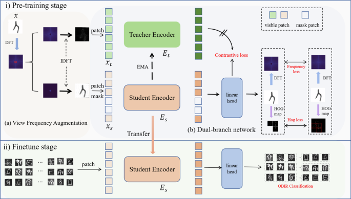
The overall structure of the proposed network.

Full size image

View frequency augmentation

Operations such as blurring and downsampling in the spatial domain are common view augmentation methods in self-supervised learning. Recent research shows that frequency domain information also has significant application potential. After an image is transformed into the frequency domain through a two-dimensional discrete Fourier transform (DFT), processing the high-frequency and low-frequency components can serve as a novel augmentation strategy. In our approach, we utilize high-frequency information to capture the edges and contours of the image, and low-frequency information to represent the details and textures. By separating the high-frequency and low-frequency information and combining it with contrastive learning for augmentation design, the model can more effectively utilize different features and achieve more robust feature learning results. Specifically, DFT can be employed to convert input OBIR image (xin {{mathbb{R}}}^{Ctimes Htimes W}) into frequency maps F(x). The formula can be formed as follows:

where f(x, y) represents the pixel value at (x, y), and F(r, i) represents the frequency value at (r, i).

We center the frequency map to obtain ({F}_{{{center}}}=F(r-frac{H}{2},i-frac{W}{2})), and then mask the central region to obtain the high-frequency and low-frequency maps, respectively. When masking the frequency map, a circular masking approach can be adopted. Specifically, define the masking matrix as (M={left{0,1right}}^{Htimes W}). If the Euclidean distance of a frequency point from the center of the frequency map is less than a certain threshold δ, its value is set to 1. Otherwise, it is set to 0. The formula can be formulated as follows:

where (c_m, c_n) represents the center of the rubbing.

Subsequently, the masking matrix and the centered frequency map are multiplied element-wise. The inverse discrete Fourier transform (IDFT) is applied to transform the resulting frequency map back to the spatial domain to obtain the high-frequency image ({x}_{{ {fre}}}^{{ {h}}}) and the low-frequency image ({x}_{ {{fre}}}^{ {{l}}}). The formula is defined as follows:

where 1 is the all-ones matrix.

Finally, the selection of images by the encoder is randomized during real training. the student encoder handles low-frequency images, and the teacher encoder handles high-frequency images for descriptive convenience, as shown in Fig. 3. These operations are not only an augmentation but also introduce a frequency domain reconstruction task to the model, which enhances the learning and generalization capabilities of our OBI-CMF.

Dual-branch network

Student branch

The student encoder is responsible for learning information about specific views. It performs patch encoding of low-frequency image from ({x}_{{ {fre}}}^{{ {l}}}) and converts it into N patches ({x}_{{ {s}}}={[{h}_{{ {s}}}^{1},{h}_{{ {s}}}^{2},…,{h}_{{ {s}}}^{N}]}^{{rm {T}}}in {{mathbb{R}}}^{Ntimes d}), where d denotes the dimension of the patch. First, by randomly masking m patches and using all-zero parameters ({h}_{0}in {{mathbb{R}}}^{1times d}) to generate processed patches. Second, positional embeddings ({ {po{s}}}_{ {{s}}}in {{mathbb{R}}}^{(N+1)times d}) are added to each patch and class token ({ {cl{s}}}_{{ {s}}}in {{mathbb{R}}}^{1times d}) to retain its spatial information. Then, the modified patches are fed into the student encoder E_s. The encoder structure used here is based on ViT, which is also used in MAE and SimMIM. Ultimately, the encoder outputs features ({z}_{{ {s}}}={[{ {cl{s}}}_{{ {s}}},{z}_{{ {s}}}^{1},{z}_{{ {s}}}^{2},…,{z}_{{ {s}}}^{N}]}^{{ {T}}}in {{mathbb{R}}}^{(N+1)times d}). The formula is as follows:

After that, we use HOG features and frequency domain features as the targets for image reconstruction, primarily because HOG features are highly robust against damage and noise in images. Specifically, we convert the output data of the student encoder into HOG features through the HOG mapping head ξ_h to obtain more robust and reliable feature representations ({x}_{{ {h}}}in {{mathbb{R}}}^{Ctimes Htimes W}) for loss computation. Additionally, we incorporate frequency domain features as another consideration for reconstruction loss. Specifically, the features output by the student encoder are passed through a linear head ξ_f to obtain predictions ({x}_{ {{f}}}in {{mathbb{R}}}^{Ctimes Htimes W}) for frequency loss computation.

Teacher branch

The role of the teacher branch is to learn an alternative view to help the student encoder learn discriminative features. The teacher encoder has the same structure as the student encoder, but its input is the entire image. This helps our OBI-CMF learn more complete information and provides better-supervised signal to the student encoder.

Specifically, the teacher encoder E_t takes the patches ({x}_{{ {t}}}={[{h}_{{ {t}}}^{1},{h}_{{ {t}}}^{2},…,{h}_{{ {t}}}^{N}]}^{{ {T}}}in {{mathbb{R}}}^{Ntimes d}) and class token ({rm {cl{s}}}_{{rm {t}}}in {{mathbb{R}}}^{1times d}) as input, along with positional embeddings ({ {po{s}}}_{{ {t}}}in {{mathbb{R}}}^{(N+1)times d}) to obtain features ({z}_{{ {t}}}={[{ {cl{s}}}_{{ {t}}},{z}_{{ {t}}}^{1},{z}_{{ {t}}}^{2},…,{z}_{{ {t}}}^{N}]}^{{ {T}}}in {{mathbb{R}}}^{(N+1)times d}). The formula can be rewritten as follows:

Unlike the student encoder, the parameters of the teacher encoder are updated using exponential moving averaging (EMA) instead of conventional backpropagation. Specifically, the parameter update formula is as follows:

where θ_t parameter represents the parameters of the teacher encoder, and θ_s represents the parameters of the student encoder. β is a hyperparameter ranging between 0 and 1. In this paper, β is set to 0.99. The exact process is as in Algorithm 1.

Algorithm 1

Training process of our OBI-CMF

Input:x: input image; K: number of optimization steps; N: batch size;

Output:x_h, x_f: HOG features and frequency map; z_t: patches are encoded by the teacher encoder;

 1: for k = 1 to K do

 2: for i = 1 to N do

  / * transform the image to the frequency domain and centralize * /

 3:   (F={{DFT}}(x),{F}_{{{center}}}=Fleft(r-frac{H}{2},i-frac{W}{2}right))

    / * obtain high-frequency and low-frequency views * /

 4:   ({x}_{{fre}}^{{l}}={IDFT}(M(r,i)cdot {F}_{{rm {center}}}(r,i)))

 5:   ({x}_{{{fre}}}^{{h}}={{IDFT}}((1-M(r,i))cdot {F}_{{{center}}}(r,i)))

    / * select one view to input into the student encoder * /

 6:   ({x}_{{{s}}}={x}_{{{fre}}}^{{{l}}}cdot m+{h}_{0}cdot (1-m))

 7:   z_s = E_s(x_s)

  / * extract HOG features and obtain frequency domain prediction * /

 8:   x_h = HOG(ξ_h(z_s)), x_f = DFT(ξ_f(z_s))

    / * input another view into the teacher encoder * /

 9:   z_t = E_t(x_t)

    / * obtain contrastive learning loss * /

10:  Loss_Con = InfoNCE(z_t, ξ_c(z_s))

    / * training objective * /

11:  Loss = Loss_Hog(HOG(x), x_h) + Loss_Fre(x_f, DFT(x_t)) + μ ⋅ Loss_Con

12: end for

    / * update network parameters with linear headers * /

13: θ_s, ξ_h, ξ_f, ξ_c = optimize(θ_s, ξ_h, ξ_f, ξ_c, Loss)

    / * update teacher network * /

14: θ_t = β ⋅ θ_t + (1−β) ⋅ θ_s

15: end for

Training objective

Contrastive loss

In our research, we adopt InfoNCE⁴⁷ as the contrastive loss function. The expression of InfoNCE is as follows:

where (({({z}_{{ {t}}})}_{i},{({z}_{{ {t}}})}_{i}^{+})) represents positive pair, (({({z}_{{ {t}}})}_{i},{({z}_{{ {t}}})}_{i}^{-})) represents negative pair, cos(,) represents cosine similarity, τ is the temperature constant and B is mini-batch.

Reconstructive loss

In the reconstruction task, we reconstruct the HOG features and frequency domain features of the masked patches with the linear heads.

Hog loss

We convert the output x_h of the HOG linear head and the original image x to HOG features, and then we calculate the Euclidean distance of the masked regions features. The formula is defined as follows:

where HOG represents extract HOG features, m represents the masked patches.

Frequency loss

Inspired by Xie et al.³⁰, our frequency domain loss is calculated only for the part masked by the student branch and is formulated as follows:

where q and p represent our model outputs and original values at (u, v) respectively. R(r, i) and I(r, i) represent the real and imaginary parts, respectively.

The final target for our training loss is as follows:

where μ is the weight parameter for balancing the loss, which is set to 0.3, more details of the experiment are shown in Table 8.

Pre-training

Dataset

The OBC306 dataset, which is from the YinQiWenYuan (https://jgw.aynu.edu.cn/) website led by the Anyang Normal College, is utilized to evaluate the performance of our OBI-CMF. Each image is scanned from the catalog and contains only one oracle bone character. As illustrated in Fig. 2, we can see that the OBC306 dataset is class imbalanced. The most numerous class contains over twenty thousand images, while the least represented class has only one image. As depicted in Fig. 4a, the size of each image varies. To make the image size uniform, bilinear interpolation is employed to uniformly resize all images to 128 × 128 pixels as depicted in Fig. 4b. Finally, we reprocess the dataset to obtain three new sub-datasets for the balanced (OBIR-10, OBIR-100) and imbalanced (OBIR-ID) tasks.

a Original OBIR image. b Standardize OBIR image with bilinear interpolation. c Generated OBIR samples by GAN.

Full size image

OBIR-10: For the balanced data context task, the OBC306 dataset is reverse sorted, and the top 10 categories are selected based on the amount of data. 5800 OBIR samples are randomly selected for each category and divided into training and test sets with an 8:2 ratio, thus providing a robust framework for assessment. Table 1 shows some of the labels and images.

OBIR-100: Similarly, a reverse sorting process is performed for the OBC306 dataset, and the top 100 classes are selected based on data quantity. For each class, 1000 samples are chosen. For classes with over 1000 samples, 1000 samples are randomly selected. For classes with fewer than 1000 samples, GAN is employed to generate additional samples to reach 1000 per class, the generated samples are illustrated as Fig. 4c. The generated samples account for only 8% of the total samples.

OBIR-ID: For the imbalanced data context task, the top 196 classes are selected based on data quantity for the training dataset. 110 samples are randomly selected for the testing set within each class, with the remaining samples designated for training. Following Liu et al.⁴⁸, the number of OBIR samples per class in the training set is categorized as follows: classes with fewer than 100 samples are termed “OBIR-Few”, those with between 100 and 1000 samples are termed “OBIR-Medium”, and those with over 1000 samples are termed “OBIR-Many”. The details of the OBI sub-dataset are illustrated in Table 2.

Implementation details

We utilize ViT-base/16 as the backbone and apply a circular mask with a radius of 8 to the frequency images. Then, Our OBI-CMF is trained on the three sub-dataset of the OBC306: OBIR-10, OBIR-100, and OBIR-ID. Our network is implemented with PyTorch V2.1.2 using a single GeForce RTX 4090 GPU for all experiments. A pre-training phase for 300 epochs is conducted on the training set, following the ViT structure settings like BEiT²⁷. The training process involves resizing images to a resolution of 128 × 128, with a batch size of 128. For optimization, the AdamW optimizer is employed with betas (0.9, 0.95) and a weight decay of 0.05. The base learning rate is 3 × 10⁴. After pre-training, we finetune the trained student encoder for 100 epochs on the OBIR classification task.

Evaluation for OBI classification

OBI classification on balanced datasets

OBI classification on OBIR-10

To evaluate the classification performance of our model, the performance comparison between our OBI-CMF with some supervised and self-supervised methods is depicted in Table 3. Among them, the self-supervised learning methods we compare include contrastive learning methods (e.g., SimSiam³², MoCov3³³) and masked reconstruction-based methods (e.g., MAE²⁶, MFM³⁰). As suggested in Table 3, our model achieves the best results with 99.57% at Top-1 and 99.98% at Top-5, surpassing the best-supervised model, DenseNet¹⁹, which achieves 99.46%, as well as outperforming all self-supervised methods listed in Table 3. The experimental results indicate that our OBI-CMF effectively captures essential features, excelling particularly on small, balanced datasets, emphasizing the importance of contrastive learning and frequency domain reconstruction.

To better understand the capability of our proposed model, the confusion matrix of our OBI-CMF classification performance on OBIR-10 is presented in Fig. 5. As exhibited in Fig. 5, most of the samples are correctly categorized into the true category to which they belonged. For example, 1160 of the samples with a true label of 0 and 8 (and) were correctly predicted to be in category 0 and 8 (and), which indicates a better overall performance of the OBI-CMF. Meanwhile, we show the learning curve of the training results in Fig. 6. Figure 6 shows that although the test loss is high initially, the loss of our method decreases quickly, and the final result is optimal. This suggests that our model effectively learns more adequate features in the pre-training phase, improving the ability to recognize complex OBIR samples accurately.

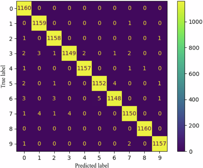
Confusion matrix of OBI-CMF classification performance.

Full size image

Learning curve during fine-tuning.

Full size image

OBI classification on OBIR-100

Compare our method with the existing methods using the OBIR-100. We can measure the performance of our OBI-CMF on a larger dataset. After pre-training on the training set, the trained student encoder is fine-tuned on the test set for the OBI classification task. To make the MFM³⁰ better suited to our task, we reduced the radius of the frequency-domain circular mask from 16 to 8.

As depicted in Table 4, our OBI-CMF achieves the highest Top-1 accuracy of 95.08%, which suggests our method can boost the ability of the feature extractor. Our method achieves the best fine-tuned performance on OBIR-100. Specifically, it outperforms the supervised method DenseNet¹⁹ by 0.68% and the self-supervised method MFM³⁰ by 0.22% in terms of Top-1 accuracy. The results indicate that our method can attain a comparable performance with the state-of-the-art supervised methods and self-supervised methods. Through this series of experiments, the superior performance of our method can be demonstrated when dealing with large balanced datasets, and its potential can be shown in OBI classification tasks.

To evaluate its performance on difficult samples with large inter-class differences and noise, we compared our OBI-CMF with MAE²⁶ and MFM³⁰, as illustrated in Fig. 7. The experimental results show that OBI-CMF is able to capture the global details better than MAE²⁶ and MFM³⁰, and exhibits stronger feature extraction capabilities. Especially when facing images with large inter-class differences, our model is able to distinguish different classes effectively. The analysis of the combined accuracy shows that OBI-CMF still maintains a high performance when dealing with these difficult samples, and successfully distinguishes the input OBIR (Fig. 7a). Ultimately, the prediction results of OBI-CMF (Fig. 7e) are highly consistent with the real labels (Fig. 7b), which further proves that our model is still able to extract accurate and representative features despite the significant noise and inter-class differences. However, when dealing with OBIRs that are heavily affected by noise achieving better differentiation poses a significant challenge for the model.

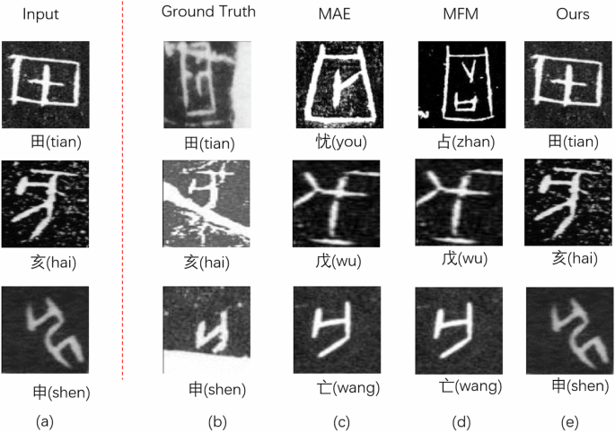
a The easy-to-distinguish samples in the class. b the hard-to-distinguish samples in the class. c–e represents the classification results of MFM, MAE, and our model.

Full size image

OBI classification on imbalanced dataset

Self-supervised learning consists of two stages. Not relying on labeled data in the pre-training phase can effectively alleviate the trouble caused by label imbalance. We compare our OBI-CMF with previous supervised and self-supervised methods on the OBIR-ID to validate the features learned by the model, based on the imbalanced nature that exists in the OBI dataset.

The results are illustrated in Table 5, our method achieves 88.66% in overall accuracy, which outperforms the supervised method DenseNet¹⁹ by 0.89% and all self-supervised methods listed in Table 5. In more detailed metrics, our method achieves 95.12%, 90.07%, and 71.17% in OBIR-Many, OBIR-Medium, OBIR-Few, respectively. From the above results, it can be seen that our method improves the accuracy of OBIR-Few without losing the accuracy of OBIR-Many at the same time. This shows that our OBI-CMF not only learns adequate feature representation but also takes into account the imbalance that exists in the dataset.

Ablation study

In this section, we conduct detailed experiments on each module and parameter of the OBI-CMF to further analyze and validate its performance. These experiments are conducted based on the OBIR-100 dataset. By tuning and testing different modules and parameters, we can study the impact of each component on the overall model performance. Our model structure and parameter settings are then optimized to obtain the best classification results.

Effectiveness of module

To validate the impact of each module on the performance, we conduct several experiments to test the effects of different modules individually. As depicted in Table 6, the Top-1 accuracy of our model improved by 0.1% each after adding the HOG reconstruction task and the comparison learning task, respectively. This indicates that these two modules positively contribute to our model.

Therefore, we integrate both the HOG reconstruction task and the contrastive learning task into the model. The experimental results confirm that our approach achieves the highest accuracy, which further validates the importance of these two modules in improving model performance. In summary, these experimental results demonstrate the contribution of each module to the model performance and the effectiveness and robustness of our approach.

Effectiveness of different targets

Pixels have been widely used to reconstruct targets in previous studies due to their intuitive and easy implementation. Similarly, we compare the results of reconstructing pixels and reconstructing HOG features. The results show that pixel reconstruction leads to a decrease in model performance. This is due to the large amount of noise present in the OBI image. Restoring the pixels alone interferes with the learning process of our OBI-CMF.

As shown in Table 7, HOG features can mitigate noise and other distractions in the image and provide a more robust feature representation. Therefore, we choose HOG features as the reconstruction target. This choice improves the learning efficiency and classification accuracy of the model and further validates the superiority of HOG features in processing OBI images.

Effectiveness of balance parameter μ

The reconstruction task and contrastive learning in self-supervised learning are applied simultaneously in our OBI-CMF. Therefore, we introduce the hyperparameter μ to balance these two losses in Eq.10. We set μ to 0.1,0.3,0.5 in our experiments.

As depicted in Table 8, our OBI-CMF performs best with a μ value of 0.3. Either we are increasing or decreasing μ leads to a decline in model accuracy. This observation emphasizes the importance of a balanced integration of contrastive learning and reconstruction tasks to effectively enhance the feature learning capabilities of our model from OBI images. Then, we identify optimal parameter settings that allow the model to achieve optimal performance by effectively balancing these two tasks.

Effectiveness of mask radius

In previous image classification tasks, a common practice is to use an image size of 224 × 224. However, we have adopted a smaller image size of 128 × 128 for our study. Consequently, we adjust the masking radius in the frequency domain to accommodate this change in resolution.

Table 9 reveals that a masking radius of 16 significantly reduces the model accuracy. This indicates that a masking radius that is too large can damage the integrity of the image content and hinder the model’s ability to learn features. On the other hand, a masking radius of 4 also reduces the accuracy of the model, suggesting that the task might be too easy for the model to extract sufficient features. Therefore, we chose a more moderate masking radius to ensure our model can adequately capture essential features in the OBIR images, thereby improving classification accuracy. Following this adjustment, the performance of our model in processing OBIR images is optimized and ensured by the effectiveness of our OBI-CMF in OBI classification tasks.

Conclusion

In this paper, we present a simple yet effective self-supervised OBI recognition method named OBI-CMF. Our OBI-CMF integrates HOG feature reconstruction to mitigate the effect of image noise on the model’s ability to learn image features. In addition, the model performance is significantly enhanced by employing a mutual supervision mechanism between the frequency and spatial domain information. To further enhance this performance, our approach is complemented by contrastive learning, specifically aimed at improving the model’s capability to discriminate between intra-class variants of OBI images. Our OBI-CMF demonstrates excellent robustness and achieves compelling results under diverse conditions by comprehensively evaluating balanced and imbalanced datasets. Although our OBI-CMF achieves excellent performance, there are still some factors that need to be further investigated. In the future, we will deal with the problem of the large amount of noise in the image of the OBIR. The existing Oracle knowledge will then be utilized to migrate to unrecognized OBI to help decipher unknown rubbings. Finally, we hope that our work can provide a valuable tool for Oracle interpretation work.