Interpretable material descriptors for critical pitting temperature in austenitic stainless steel via machine learning
Introduction
Austenitic stainless steel, with its high chromium and nickel content, maintains a stable austenitic microstructure at room temperature, endowing it with remarkable corrosion resistance and mechanical properties1,2. Its corrosion resistance is derived from a passive chromium oxide layer, which renders it resistant to rust and degradation in aggressive environments3,4. It is deemed indispensable in various engineering application scenarios, including nuclear, marine, aerospace sectors, etc5,6. However, despite its numerous advantages, austenitic stainless steel still faces challenges associated with localized corrosion, particularly pitting corrosion, which poses a significant threat to structural integrity and service reliability7. Understanding the facile factors behind pitting corrosion and developing effective solution strategies are identified as both challenges and opportunities for enhancing the performance and service life of austenitic stainless steel in diverse applications.
The critical pitting temperature (CPT) has been recognized as a crucial parameter in assessing the susceptibility of metal structural materials to pitting corrosion. It represents the temperature threshold beyond which localized corrosion is initiated and signifies the transition from metastable to a steady state of pitting. Since the concept of CPT was introduced, extensive studies have been conducted to explore its relation with alloy composition and interpret it through different physical models. For example, to investigate the influence of alloying elements N, Mo, and Mn on the pitting corrosion resistance, Jargelius-Pettersson8 conducted the pitting resistance of high alloyed austenitic stainless steel with varying contents of those alloying elements. The results revealed the synergistic benefits of Mo and Ni, as well as the detrimental effects associated with Mn alloying. To examine the pitting corrosion behavior of super austenitic stainless steel, Meguid et al.9 investigated the CPT of 254SMO stainless steel in the sodium chloride solution. It was found that the CPT decreased with chloride content decrease, and the critical pitting potential exhibited a linear relationship with the logarithmic concentration of chloride ions above the CPT. In the view of the distribution range of CPT values for 316 L stainless steel increased with the decrease of the aggressiveness of exposure condition, Li et al.10 proposed a CPT model with the assumption that the maximum dissolution current density of pitting equals or surpasses the critical diffusion current density. Nonetheless, the intricate interplays among the different components of austenitic stainless steel and their correlations through physical models pose significant challenges in elucidating the underlying mechanism of CPT.
Recently, machine learning technique has emerged as a valuable tool in the field of material corrosion11,12, facilitating the prediction and analysis of phenomena such as potentiodynamic polarization curves13,14, corrosion rates15,16, pitting potentials17,18,19, etc. This technological advancement has substantially contributed to the deeper understanding of corrosion processes. For instance, to predict the corrosion rate of low alloy steel in marine environments, Diao et al.15 developed a machine learning framework employing gradient-boosting decision tree (GBDT) and Kendall correlation analysis. Thermal conductivity and electronegativity were identified as critical atomic features influencing the corrosion rate. To analyze the stochastic nature of the localized corrosion current distribution in 316 L stainless steel under sodium chloride solution, Coelho et al.13,20 employed linear regression and artificial neural network (ANN) techniques to derive pitting corrosion descriptors. A higher correlation was observed in estimations based on the conditional median of the log(j) versus E curves compared to that of the conditional mean. To elucidate the variation in pitting potential with different alloy compositions, Song et al.17 employed interpretable machine-learning techniques. A pitting potential prediction model was validated, and the detailed influences on pitting potential were discussed. Integrating machine learning models with interpretability algorithms presents a promising pathway for enhancing the understanding and accurate prediction of corrosion phenomena. Unfortunately, there are currently relatively few machine learning studies on CPT.
In this work, a database on the CPT in austenitic stainless steel is collected from extensive scientific literature. It includes a dataset of 148 atomic and physical property features, which are derived from chemical composition attributes through various calculation methods21. To address the dimensionality challenges posed by the high dimensionality of such datasets, an optimized feature selection strategy is introduced. Subsequently, a quantitative relationship between critical descriptors and CPT is validated through interpretive analysis and symbolic regression methods.
Result and discussion
In this study, two distinct strategies are introduced to predict the CPT in austenitic stainless steel accurately, as depicted in Fig. 1. The influence of alloy composition and testing conditions on CPT has been extensively documented in literature8,9, underscoring the importance of establishing a relationship between these factors and CPT to design pitting-resistant alloys. Strategy I proposes a direct modeling approach that utilizes experimental data on composition and testing conditions from existing studies to analyze their influence on CPT. To reduce the curse of dimensionality and avoid overfitting, Strategy II develops an optimal approach based on the atomic and physical features. This approach significantly expands the dataset based on the alloy compositions by incorporating corrosion-related atomic features and employing various computational methods. Considering these features as intrinsic properties of the alloys, this strategy aims to enhance the understanding of the CPT concept.
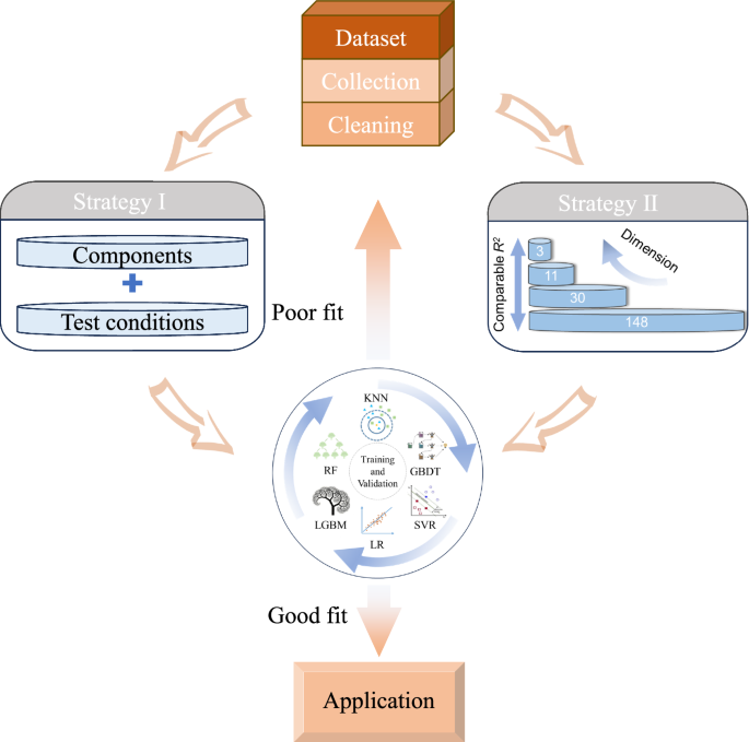
Strategy I: developing machine learning models based on composition and test condition data from the original dataset. Strategy II: constructing a machine learning model based on atomic and physical features derived from composition features.
Strategy I
Firstly, seven machine learning models based on 11 component features and 6 test condition features are developed, and their predictive performance is evaluated using ten-fold cross validation, as shown in Fig. 2a, b. The accuracies of these models range from 0.955 to 0.976, while the prediction RMSE decreases inversely from 5.984 to 4.424 °C. The GBDT model emerges as the optimal prediction model, with results depicted in Fig. 2c, wherein the predicted values are aligned along a 45° diagonal with the experimental values, indicating a basic consistency between the CPT prediction results and the experimental findings. Subsequently, the feature importance ranking based on Strategy I could be derived from the GBDT model, as shown in Supplementary Fig. 1. It indicates that in austenitic stainless steel under a chloride ion environment, the CPT is significantly influenced by elemental features, particularly by elements Cr, Ni, Mo, N, Mn, and Cu. It should be emphasized that under some other environmental conditions, such as scan rate10, roughness22, heat treatment23,24 and the presence of corrosion inhibitors25,26, may also influence CPT.
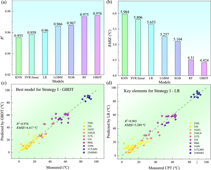
Comparison of (a) R2 and (b) RMSE across different machine learning models, and the prediction results of (c) an optimal machine learning model GBDT and (d) a linear regression model based on corrosion-resistant alloy elements. The colors represent the numbering of different austenitic stainless steel grades, and ‘LR’ in the figure represents a linear regression.
Inspired by the formula of PREN8,27 that a linear relationship between key alloy compositions and pitting resistance, the features importance screening and CPT are subsequently elucidated through linear regression analysis. The predicted results are illustrated in Fig. 2d, with the expression of the linear model shown in Eq. 1:
Equation 1 is similar to the CPT formula summarized in literature28,29, indicating consistent results for CPT in austenitic stainless steel. It is noteworthy that in austenitic stainless steel under a NaCl solution, the prediction accuracy of the composition-based linear regression model (R2 = 0.965) is observed to differ only slightly from that of the GBDT model, which is based on composition and testing conditions (R2 = 0.976). Nonetheless, each composition is not simply linear proportional to the corresponding CPT, as shown in Supplementary Fig. 2, wherein different composition regions exhibit varied effects on CPT30. Additionally, within the widely recognized SBN model31, CPT is considered as the intersection point of the critical diffusion current density of metal cations in the salt film and the maximum dissolution current density of the dissolution of the pitting matrix as a function of temperature variation. Establishing a connection between the PREN and the SBN model for CPT prediction presents challenges. Machine learning predictions incorporating atomic and physical features might provide new insights into addressing this complexity.
Strategy II
Subsequently, an analysis employing Strategy II is conducted to assess the influence of atomic and physical features on the CPT, which is considered to be closer to the intrinsic properties of CPT. Among the 148 features analyzed, numerous features exhibit a high correlation but exert a weak effect on CPT. To balance the accuracy and efficiency of the machine learning model, a multi-stage feature screening scheme is adopted, as shown in Fig. 3a. Firstly, the importance coefficient, average absolute SHAP value, and variance of each feature are calculated, as illustrated in Fig. 3b, which reflects the feature importance and data informativeness. In this work, features are filtered out if their importance coefficient for CPT falls below 0.002, their average absolute SHAP value is under 0.200, or the logarithm of their variance is below -12.000. The selection criteria, referred to as the “three-standard selector”, are illustrated within the rectangle box in Fig. 3b, where the features that meet these criteria are highlighted and subsequently selected. The “three-standard selector” is established to ensure that the features retained for model development represent approximately the top 80% of all features in terms of their influence on CPT, as determined by the combined metrics of importance, variability, and SHAP values. This methodology guarantees that the selected features are not only among the most influential but also maintain statistical significance regarding their variance and contribution to the predictive accuracy of machine learning models. The feature dimension is significantly reduced from 148 to 30 (Fig. 3a), with only 20% of all features being features, whereas accuracy slightly increases from 0.970 to 0.974, thereby reducing the overfitting of the machine learning model.
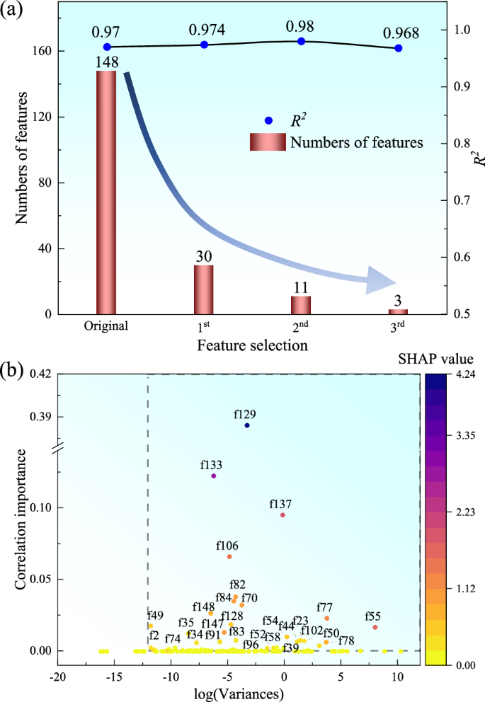
a The screening process of 148 physical features, and (b) the application of the “three-standard selector”, which includes the correlation importance, the data variance, and the average absolute SHAP values. The criteria outlined in the rectangle box is: correlation importance > 0.002, log (variance) > −12.000, and mean ( | SHAP | ) > 0.200.
Considering that some features in the dataset of this study do not satisfy the linear and normal distribution assumptions required for the PCC, as illustrated in Supplementary Fig. 3, the Spearman correlation coefficient is adopted for further feature correlation analysis due to its ability to handle intrinsic nonlinearity16. The heatmap of the 30 retained features calculated via the Spearman method is shown in Fig. 4, wherein an intensification of the blue color indicates an increase in positive correlation between features (up to +1), whereas an intensification of the red color signifies an increase in negative correlation (up to −1). Features with absolute correlation coefficients higher than 0.8 in heatmap analysis are categorized together, as depicted by the brown rectangular box in Fig. 4, wherein only the most important feature within this category is retained. Following this correlation analysis, the number of features is further reduced from 30 to 11, whereas the accuracy of the machine learning model prediction slightly increased to 0.980.
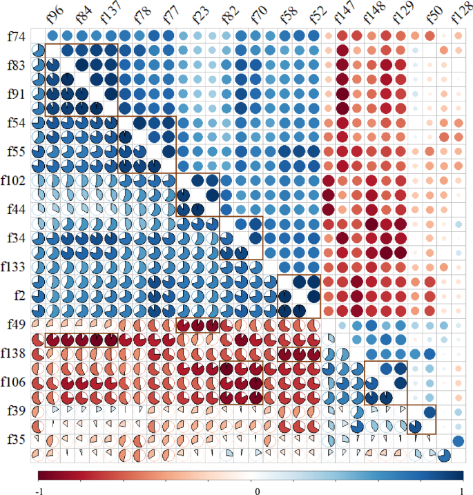
The heatmap of the 30 features remained after the “three-standard selector” process.
Based on the “three-standard selector” and subsequent correlation analysis, the optimal subset method is utilized to enumerate all 2047 combinations of the 11 retained features. The prediction accuracy R2 of the linear regression model for each combination varies with the number of features (Fig. 5a), and the RMSE varies with the number of features (Fig. 5b). The magenta dots represent the prediction results of the best feature combination for the number of features, whereas the gray dots represent the prediction results of all combinations. When the features count is reduced to three, both the maximum prediction accuracy R2 and the minimum RMSE achieve their relative optimal values, identifying ({E}_{max }), (lambda), and ({{VEC}}_{{sum}}) as the optimal feature set. The feature selection process of the optimal subset ultimately reduces the feature count to three, whereas the prediction accuracy of the GBDT machine learning model remains around 0.968, as illustrated in Fig. 3a, which evidences the effectiveness and reliability of the feature engineering process.
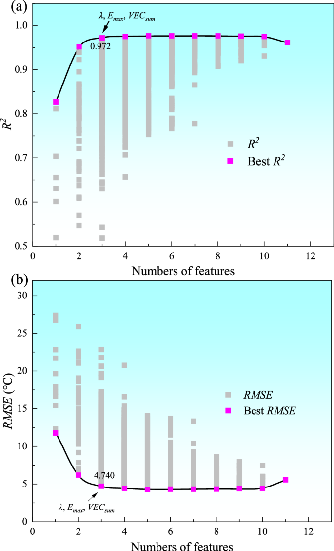
a The prediction accuracy and (b) the RMSE for all combinations from the optimal subset screening. Magenta represents the optimal prediction result for a given number of features.
For the three selected features, ({E}_{max }), (lambda), and ({{VEC}}_{{sum}}), further investigations are carried out on the training and optimization of various machine learning models using ({{VEC}}_{{sum}}), and the results of their prediction accuracy R2 and RMSE are displayed in Fig. 6a. The prediction accuracies of all machine learning models are generally above 0.946, and the RMSE is below 6.577 °C, indicating the predictive robustness of the selected three features. As the optimal machine learning model, the scatter plot of the random forest model is shown in Fig. 6b. A high prediction accuracy of 0.974 and an RMSE of 4.606 °C demonstrate good consistency between the prediction and the experimental results of CPT. Consequently, the CPT prediction model based on Strategy II not only effectively reduces the number of features and minimizes the risk of overfitting, but also significantly improves the interpretability of the CPT model. Furthermore, the dataset is divided into training, validation, and test sets using a ratio of 7:1:2, as illustrated in Supplementary Fig. 4a. The accuracy of the test set (0.976) is found to be in close agreement with the cross-validation accuracy (0.974), despite slightly lower than the validation set accuracy (0.983). This consistency validates the robustness of the cross-validation method and demonstrates the generalization performance of the Random Forest model. In the chloride ion solution of austenitic stainless steel, which is the focus of this work, it is observed that the influence of alloy composition on CPT is predominant. In contrast, the influence exerted by the testing environment and conditions on the collected data is found to be relatively weak. It is confirmed by CPT studies (the linear regions 1, 2 and 3 shown in Fig. 6b) of steel samples with the same composition under varying testing conditions. The linear regression prediction correlating the testing conditions and CPT is depicted in Supplementary Fig. 5. This figure illustrates the relationships between CPT and various factors: in Region 1, the correlation of pressure and dissolved oxygen content; in Region 2, the correlation of Cl–, pH, and pressure; and in Region 3, the correlation of Cl– and pH. It is worth mentioning that the variations in CPT are influenced by multiple factors, such as the testing conditions shown in Supplementary Fig. 5, the selection of the temperature gradient during the experiment, the precise determination of the Z-curve position, and the inherent uncertainties associated with pitting corrosion. Above all, further systematic research is required to investigate the influence of more detailed and extensive environmental conditions on CPT.
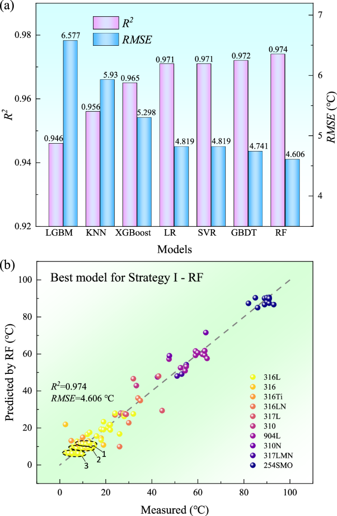
a Comparison of prediction results of various machine learning models, where the red label represents R2, the blue label represents RMSE, and (b) prediction results of the optimal model random forest, where the colors represent identifiers of different austenitic steel grades and “RF” in the figure represents random forest regression.
Machine learning models are often referred to as “black box models” due to their lack of representation through the physical formula and intuitive visuals. To further elaborate, a SHAP analysis based on the optimal random forest model is conducted to assess the effect of the three features of ({E}_{max }), (lambda), and ({{VEC}}_{{sum}}) on the CPT data. The SHAP scatter plots are displayed in Fig. 7a–c. ({E}_{max }), (lambda), and ({{VEC}}_{{sum}}) all exhibit a roughly negative correlation with CPT, with ({E}_{max }) having the most considerable effect on CPT, followed by ({{VEC}}_{{sum}}) and (lambda). Figure 7d illustrates the respective linear relationship between the SHAP values for ({E}_{max }), (lambda), and ({{VEC}}_{{sum}}), and the experimental CPT measurements across a range of austenitic stainless steels with varying alloying compositions. The error bars represent the range of SHAP values and experimental CPT values for different degrees of alloying. The relationship between the SHAP values for ({E}_{max }), (lambda), and ({{VEC}}_{{sum}}) and CPT demonstrates the robustness of SHAP additive explanatory analysis.
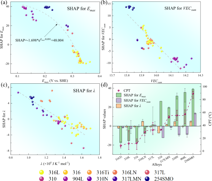
The scatter of (a) SHAP values for ({E}_{max }) with ({E}_{max }), (b) SHAP values for ({{VEC}}_{{sum}}) with ({{VEC}}_{{sum}}), and (c) SHAP values for λ with λ, with the colors representing the numbering of steel grades with different degrees of austenitic stainless steels. And (d) a comparison of the strength of the influence of ({E}_{max }), ({{VEC}}_{{sum}}) and λ on CPT based on SHAP analysis. The error bars in the figure represent the range of values for the corresponding SHAP or CPT in the corresponding steel grade.
The symbolic regression method provides a powerful tool for exploring the quantitative relationship between various descriptors and the corresponding CPT32,33. Based on the SHAP analysis of three selected features, a quantitative relationship (Eq. 2) between the three features (({E}_{max }), (lambda), and ({{VEC}}_{{sum}})) and CPT is derived through symbolic regression analysis,
The prediction results of Eq. 2 are shown in Fig. 8, where the notable prediction accuracy (R2 = 0.972) underscores the efficacy of the potential model derived via symbolic regression, consistent with the results from the random forest model. A negative correlation is observed between the three selected features and the CPT, which is consistent with the SHAP scatter plot (Fig. 7). Moreover, the influence of ({E}_{max }) on CPT is identified as the most substantial, followed by ({{VEC}}_{{sum}}) and (lambda), which is also consistent with the SHAP analysis. The generalization performance of the symbolic regression model was further validated by dividing the data into training, validation, and test sets, with corresponding proportions of 70%, 10%, and 20%. As shown in Supplementary Fig. 4b, the accuracy of the validation set (0.975) is found to be in close agreement with the cross-validation results (0.972).
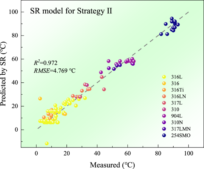
“SR” in the figure denotes symbolic regression.
Figure 9a, b show the combined effects of ({{VEC}}_{{sum}}) and ({E}_{max }), as well as ({{VEC}}_{{sum}}) and (lambda), on the corresponding CPT, respectively, with CPT values exhibiting a gradient from blue to red. As ({E}_{max }), (lambda) or ({{VEC}}_{{sum}}) increase, a decreasing trend in CPT values is observed, consistent with the trend analyzed by the heatmap (Fig. 4) and SHAP analysis (Fig. 7). Notably, the colored regions in Fig. 9 represent the distribution areas of the corresponding experimental data, while the surrounding blank areas are filled with white (or null values) due to the absence of supporting experimental data. The pitting process is characterized by variations in potential, and the relationships among corrosion potential, metastable pitting potential, and pitting have been widely reported18,34,35. ({E}_{max }) is defined as the weighted average of the highest standard reduction potential present in the alloy composition, representing the driving force of the corrosion reactions in the alloy, and is closely related to the pitting process. The relationship between corrosion potential and ({E}_{max }) could be illustrated by Evans diagram, as shown in Supplementary Fig. 6. As ({E}_{max }) increases, the corrosion current shows an increasing trend while the corrosion potential exhibits a decreasing trend, indicating a gradual deterioration in corrosion resistance. Therefore, the general negative correlation between ({E}_{max }) and the degree of pitting could be inferred from the literatures35,36.
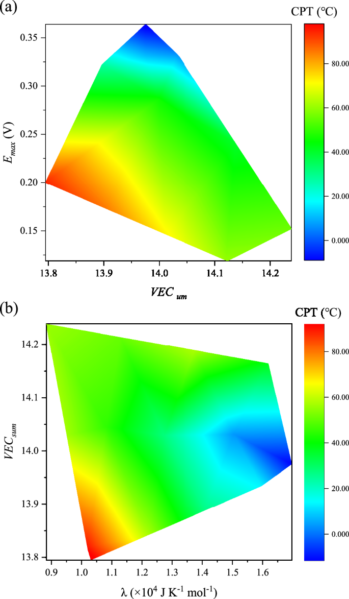
The effect of (a) ({E}_{max }) and ({E}_{max }), (b) ({{VEC}}_{{sum}}) and λ on CPT.
({{VEC}}_{{sum}}), similar to the commonly mentioned concentration of valence electrons, is defined as the number of valence electrons within a specified mass of stainless steel, affecting the probability of binding between the matrix and corrosive ions such as Cl– or O atoms18. The relationship between ({{VEC}}_{{sum}}) and pitting of alloys could be confirmed by pitting corrosion data of stainless steel with similar components37, as shown in Supplementary Fig. 7a, b. (lambda) is identified as a geometric parameter and defined as the ratio of ({Delta S}_{{mix}}) to the square of (delta)17, has been frequently discussed as a metric describing lattice stress in high entropy alloys18,38. Similarly, the negative proportional relationship between (lambda) and pitting resistance could also be derived from the analysis of Supplementary Fig. 7c, d.
CPT is widely regarded as the point where the maximum dissolution current density of pits intersects with the critical diffusion current density of electrolyte from the pit to the bulk solution with respect to temperature10,31. Given the inherently stochastic nature of pitting, the experimentally measured CPT could be considered as a statistical average of numerous pits based on the physical model39,40. In the context of austenitic stainless steel exposed to a NaCl solution, the CPT is observed to strongly correlate with the material composition8,27. This is probably because the measurement of CPT results from a dynamic equilibrium between the initiation and repassivation of numerous pits, with typical statistical properties10,40. Compared to the potentiostatic method, the potentiodynamic method may yield a more stable CPT41. The thermodynamic factor (({E}_{max })), geometric parameter ((lambda)) and valence electronics (({{VEC}}_{{sum}})) discussed in this work could be considered as a commendable descriptors of these statistical features.
In summary, this study aims to predict the CPT in austenitic stainless steel via machine learning, with a particular focus on feature interpretability. Further insights into the relationship between material descriptors and CPT are explored through two distinct strategies. Strategy I emphasizes the importance of alloy composition by constructing machine-learning models that accurately predict CPT within the collected data, particularly for austenitic stainless steel under a NaCl environment, consistent with existing observations. Strategy II identifies three crucial features, ({E}_{max }), (lambda) and ({{VEC}}_{{sum}}), whose influences on CPT are elucidated through SHAP analysis. Additionally, a quantitative expression derived from symbolic regression is utilized for the high-precision prediction of CPT, providing new perspectives for the physical interpretation of CPT. In the future, the focus of research will be directed towards enhancing the generalizability of the machine learning model. This will be achieved by extending its application to more types of steel, including ferritic and martensitic stainless steels, among others. Transfer learning techniques will be utilized to adapt the model to the unique characteristics of these materials, ensuring its accuracy and reliability42. Furthermore, the integration of experimental datasets will further strengthen the model and provide deeper insights into the effects of various features on CPT across different microstructures.
Methods
This study focuses on applying two distinct machine-learning strategies for accurately predicting the CPT in austenitic stainless steels. Strategy I employs traditional prediction methods based on composition and test conditions, and incorporates a comparative analysis with previous reports. Conversely, Strategy II constructs an extensive dataset of atomic and physical features derived from the alloy compositions. Subsequent feature selection and optimization are executed through various effective techniques. The final retained features are subjected to both interpretability analysis and quantitative regression analysis.
Dataset collection
Several experimental methods have been utilized to determine the CPT, including the immersion test27, potentiodynamic method27,41, and potentiostatic method8,41. Specifically, the immersion method, typically conducted in the solution of 6 wt.% FeCl3 and 1 wt.% HCl, requires the samples to be exposed to varying temperatures for 24 hours to detect pitting occurrence, thereby establishing the corresponding CPT27. However, this method is currently less favored due to the extended testing duration and subjectivity in pitting determination. Electrochemical techniques are preferred because of their effectiveness in quickly and accurately capturing the different stages of pitting corrosion. The potentiodynamic polarization method entails scanning samples at various temperatures to determine the pitting potential, resulting in the construction of a pitting potential versus temperature profile, known as the Z-curve, which facilitates CPT determination based on the sudden changes in potential. And the potentiostatic method applies a fixed potential to the sample while incrementally increasing the temperature, defining CPT as the temperature where a sustained current density exceeds 100 μA cm−2, typically. Despite its simplicity and widespread adoption, the potentiostatic method faces significant uncertainty, possibly due to interference by the critical crevice temperature43 or inherent methodological ambiguities10,41. Consequently, considering the importance of data richness and reliability, the CPT dataset in this work is collected from relevant literature sources28,29,34,41,44,45,46,47,48,49,50,51,52, mainly utilizing the potentiodynamic method for low Mn austenitic stainless steel in a NaCl environment.
This dataset comprises a total of 123 pieces of austenitic stainless steel tested by the potentiodynamic method, including 11 element features (C, Si, Mn, P, S, Cr, Ni, Mo, N, Ti, Cu) and 6 test condition features (chloride ion concentration, solution pH, surface roughness of test samples, pressure, dissolved oxygen (DO), electrochemical scan rate, as shown in Supplementary Table 1. The mean value (Ave), maximum (Max), minimum (Min), standard deviation (Std), and median (Med) of these features are shown in Supplementary Table 2. Regarding missing values in the dataset, the following procedures are implemented. Missing values for elements, such as Cu, Ni, and N, are replaced with the average values of the corresponding alloy standards53. For test conditions, missing values for Cl– concentration and dissolved oxygen are filled with 0. The missing values for pH and pressure are filled with a general value of 7 and 1 atm (one atmosphere), respectively, whereas missing values for surface roughness and scanning speed are filled with the minimum values observed in the dataset. These approaches ensure consistency and provide a standardized basis for further dataset analysis.
It is noteworthy that the titanium (Ti) content in the data table is predominantly recorded as zero, and there are few reports in literature regarding the influence of Ti on CPT. Moreover, the influence of Ti on pitting corrosion is still controversial54,55. The effects of dissolved oxygen and pressure on CPT appear to be largely represented by general values, which may be related to the standard testing procedures for CPT. Under normal testing conditions, the oxygen concentration is typically within the range of 5–15 ppm, wherein the stainless steel surface is believed to have undergone sufficient passivation, rendering it less influenced by dissolved oxygen levels56,57.
Furthermore, the heat treatment processes and the material microstructure also affect CPT, as highlighted in several studies. However, within the current machine learning framework, the available heat treatment parameters seem to exhibit considerable uncertainty, and the microstructural features and precipitate characteristics closely related to heat treatment remain challenging to quantify effectively. Considering the robustness of the machine learning model, the literature data utilized in this study is primarily sourced from commercially produced stainless steel samples that adhere to the relevant steel standards. This methodology is expected to effectively mitigate the influence of heat treatment processes on the model performance, while also ensuring the generalization performance and its applicability in guiding material research. It is essential to conduct broader studies on pitting resistance under various influencing factors in the future and to develop more advanced artificial intelligence methods that incorporate morphological approaches for a more detailed and in-depth exploration of CPT.
Xenonpy21 provides a convenient method to construct atomic features using various databases. Specifically, 58 features are sourced from Xenonpy21 and 16 features from WebElements58, along with the geometric parameters (λ) mentioned in the relevant literature, and mixing entropy (({Delta S}_{{mix}})), as well as the standard reduction potential of the corresponding element metal from the electrochemical toolbook59. The atomic and physical features are ultimately determined by various calculation methods, as shown in Eqs. (3–11), wherein ({X}_{{ave}}) denotes the weighted average of atomic molar percentages, ({X}_{{sum}}) represents the weighted sum of molar weights in a 100 g sample, ({X}_{mathrm{var}}) indicates the weighted variance of atomic mole fractions, ({X}_{{gmean}}) is the geometric mean of atomic mole fractions, ({X}_{{hmean}}) refers to the Harmonic mean of atomic mole fractions, ({X}_{{gmis}}) signifies the geometric mismatch of atomic mole fractions. The descriptions of these 148 atomic and physical descriptors are provided in Supplementary Table 3.
where ({w}_{i}) describes the molar fraction of each element component, ({w}_{i}^{* }) denotes the molar weights of each element component in a 100 g sample, ({X}_{i}) suggests the certain physical quantity of the corresponding atom, ({r}_{i}) represents the radius of the atom, (bar{r}) represents the average atomic radius.
Noteworthy, the mixing entropy ({Delta S}_{{mix}}) is frequently referenced in literature as an indicator to signify the degree of alloying in steel, representing the quality of passivation films on stainless steel17. Analogous to the formula for calculating the geometric mismatch, the parameter (delta) is utilized to quantify the degree of lattice strain. In certain single-phase alloys, a larger δ is considered to delay diffusion, thereby hindering the migration of Cl– or O atoms within the alloy, and protecting the alloy against corrosion18. Nevertheless, increased lattice strain is believed to induce significant lattice distortion and promote the formation of a second phase, adversely affecting corrosion resistance60. The standard reduction potential, defined as the potential difference between the oxidation and the reduction state of a metal, is also considered as a critical descriptor affecting the pitting of metals18.
Feature analysis
Considering the diverse ranges of various features, to facilitate the convergence of subsequent inputs into the model, and to enhance both the efficiency of feature engineering screening and the accuracy of model predictions, Eq. 12 is used in this study to normalize the feature set61.
where X denotes the feature value, ({X}_{min }) represents the feature minimum value, and ({X}_{max }) indicates the feature maximum value. Through the normalization process, the feature values are mapped to the range of [0, 1], which reduces the numerical differences between different features.
To solve the dimensionality problem by excessive features, correlation analysis is utilized as an efficient feature selection scheme. The Pearson correlation coefficient (Eq. 13) applies to data that satisfies linear and normal distribution assumptions, while the Spearman correlation coefficient (Eq. 14) is used to measure the degree of monotonicity between two characteristic variables. In contrast to the Pearson correlation coefficient, the Spearman correlation coefficient offers a broader spectrum of applicability.
where ({p}_{i}) and ({q}_{i}) mean actual value of two features, (bar{p}) and (bar{q}) mean the average of ({p}_{i}), and ({q}_{i}), respectively, ({r}_{i}), ({s}_{i}), (bar{r}), (bar{s}) represent the rank of ({p}_{i}) and ({q}_{i}) as well as the average of ({r}_{i}) and ({s}_{i}), respectively.
Machine learning algorithms
Machine learning includes a diverse spectrum of algorithms, each tailored to address specific tasks with unique strengths and application scenarios. According to the “no free lunch” theorem62, it is impractical to expect a single algorithmic model to solve all machine learning challenges effectively. Consequently, a series of regression models, including Linear Regression (LR), k-Nearest Neighbors (KNN), LightGBM (LGBM), Support Vector Regression (SVR), Random Forest (RF), Gradient Boosting Regression (GBDT) and XGBoost (XGB), are evaluated and compared via ten-fold cross-validation method, in which the best model is ultimately selected.
To evaluate the performance of various models on the dataset, a series of indexes, PCC, R2, MAE, and RMSE, are chosen in this study, as denoted by Eqs. 13, 15–17. Among them, R2 and PCC measure the strength of linear relationships. MAE measures the average deviation between predicted and actual values. RMSE is commonly used for model evaluation and accounts for the distance between predicted and actual values.
where ({y}_{i}), ({hat{y}}_{i}), (bar{y}) and (bar{hat{y}}) mean actual value, predicted value, the average of actual value, and the average of predicted value, respectively.
To accurately evaluate the prediction and generalization performance of machine learning models, the 10-fold cross-validation scheme is adopted in this work. Specifically, the entire dataset is randomly divided into ten equal parts, with each part serving as a test set while the remaining nine parts are used as the training set in a rotating manner. This process is repeated ten times, and the final reported R² value is the average of these ten validation results. To mitigate the influence of randomness inherent in the data partitioning, 50 repetitions of the entire cross-validation process for each R² calculation are conducted. Then the average of the 50 repetitions helps to smooth out any anomalies that may arise, thereby enhancing the stability and reliability of the reported results. Meanwhile, the widely used model training method of dividing the dataset into training, validation, and test sets with corresponding proportions of 7:1:2 is employed in this work to assess the robustness of the cross-validation process.
SHAP analysis, based on game theory63, serves as a powerful tool for interpreting outputs from predictive models. Each feature in a prediction is assigned a SHAP value that quantifies its contribution to the output of the model. The SHAP value analysis follows Eq. 18, with ({V}_{{base}}) as the baseline for the entire model analysis, typically determined as the mean of the target variable across all samples.
where (f({x}_{i})) represents the prediction value of the i-th sample, ({{SHAP}}_{{ij}}) denotes the SHAP value of the sample at (i-th, j-th), and (m) means the number of features.
This approach facilitates a comprehensive understanding of how individual features affect predictions, enabling researchers to discern the importance and influence of each feature within the model. By elucidating insights into feature importance and interactions, SHAP analysis contributes to refining model performance, enhancing interpretability, and guiding the feature selection processes toward optimized prediction results. Additionally, the average absolute value of all SHAPs for the j-th feature reflects the overall strength of the j-th feature in predicting the objective, serving as a measure of feature importance17,64.
To shed light on the complex mathematical relationship between selected feature variables and target variables, a symbolic regression strategy based on a genetic algorithm is adopted in this study. Symbolic regression starts with a randomly generated initial set of mathematical formulas, and then it undergoes genetic algorithm operations such as crossover and mutation, as well as evaluation of fitness functions (RMSE, MAE, etc.). This process iterates until the model closely approximates the true data distribution32,65. Through this iterative optimization, symbolic regression identifies the optimal mathematical formula, thereby facilitating an accurate prediction of the target variable. Based on the results of symbolic regression, CPT is calculated in the actual feature space of the key features. Contour maps are subsequently generated to illustrate the complex combined effects of these key features on CPT65.
Responses