Fusion of multi source data for atmospheric corrosion evaluation using sensors and image recognition
Introduction
The annual economic loss caused by steel corrosion is estimated at $2.5 trillion globally, accounting for 3% of the global gross domestic product (GDP)1,2,3,4,5. This issue is particularly critical in industries like oil and gas, where corrosion-induced structural failures can lead to major safety incidents, further increasing both economic costs and safety risks6,7. Therefore, developing techniques to accurately monitor and assess steel corrosion at an early stage is essential to reducing economic losses and improving structural safety.
In practice, manual and visual inspections remain the primary means of assessing the corrosion of materials and structures. However, these methods cannot provide detailed corrosion information and are prone to human error, often requiring validation through more precise inspection techniques8,9. Consequently, there is an urgent need for a corrosion detection method that delivers more accurate and real-time results. Currently, common corrosion monitoring techniques include the electrical resistance (ER) probe technique10, the atmospheric corrosion monitor (ACM)11,12, and electrochemical impedance spectroscopy (EIS)13,14,15,16,17,18. For instance, Wang et al. studied the evolution of rust layers on weathering steels using the ER technique19, while Yang et al. assessed the corrosion resistance on low-alloy high-strength steels with varying tin (Sn) content using EIS20.
Although machine learning models based on these monitoring techniques have enabled continuous monitoring and enhanced understanding of corrosion mechanisms, their application in practical production remains limited. One limitation is that these models are not yet sufficiently accurate for practical use. This is particularly true in complex environments where multiple variables are involved21,22,23. Additionally, the specialized equipment and technical conditions required for these methods are often unavailable in industrial settings. Furthermore, traditional models, such as the power function model, while somewhat effective under certain conditions, lack the necessary accuracy because they do not adequately account for the non-linear nature of the corrosion process. They struggle to adapt to the complexity of real-world production environments24. Therefore, it is crucial to explore new characteristics of material corrosion and to develop monitoring methods better suited for industrial applications.
In recent years, image recognition technology has been garnering significant attention in the materials field, particularly for its advantages in corrosion detection25,26,27. Image recognition techniques can visually capture changes in material surfaces during corrosion, such as variations in color, shape, and texture, allowing for the accurate detection of corroded areas28. Aijazi et al. introduced a method that uses multi-angle images to construct a 3D point cloud, which effectively detects the shape and size of corroded regions29. This approach has been particularly effective in identifying small surface changes in the early stages of corrosion, thereby improving the sensitivity and accuracy of detection. Additionally, by analyzing color changes, image processing can infer the type and concentration of corrosion products, such as the accumulation of Fe3O4 and α-FeOOH during corrosion19. Furthermore, image recognition technology is highly suitable for outdoor field inspections, as it can adapt to complex and fluctuating environmental conditions while providing comprehensive monitoring of large-area steel structures.
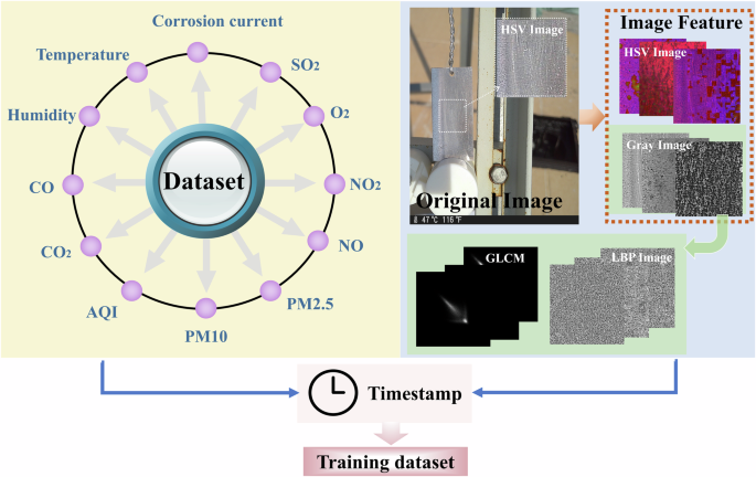
Considering these developments, we propose a novel method for detecting Q235 steel corrosion by integrating image recognition with corrosion sensor data. The goal is to rapidly assess the corrosion behavior in Q235 steel under complex environmental conditions, as illustrated in Fig. 1. First, the Contrast Limited Adaptive Histogram Equalization (CLAHE) algorithm is employed to minimize the impact of lighting variations and improve the accuracy of image analysis. Next, the image data is combined with microscopic current information obtained from a galvanic corrosion sensor, thereby integrating both macroscopic and microscopic corrosion data to comprehensively evaluate the material’s corrosion state. Machine learning algorithms are utilized to extract key corrosion features from the multi-source data. Subsequently, the corrosion degree, Qcorr, is modeled using regression analysis to provide a quantitative assessment of Q235 steel corrosion in complex environments.
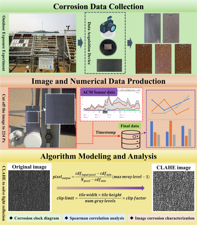
Schematic diagram of Q235 steel corrosion detection based on the fusion of image processing and corrosion sensor data.
This study proposes a novel method that integrates image recognition technology with corrosion sensor data to improve the accuracy and real-time capabilities of corrosion monitoring. The key innovations include: (1) the first-ever fusion of macro-level image texture features and micro-level current information, enabling a comprehensive assessment of corrosion states; (2) the development of an atmospheric corrosion evaluation model (Qcorr) for efficient assessment of Q235 steel corrosion under complex environmental conditions; (3) the application of the CLAHE algorithm to significantly enhance the robustness of image analysis, reducing the impact of lighting variations; and (4) the use of machine learning algorithms to extract critical corrosion features from multi-source data, substantially improving the predictive performance of the model. These advancements offer a practical and efficient new approach for corrosion monitoring in industrial environments, with broad potential for real-world applications.
Results and discussion
Analysis of corrosion sensor data
The corrosion big data clock diagram, illustrated in Fig. 2, provides a visual representation of the relative corrosion current intensity measured by sensors over a 24-h cycle. The diagram features concentric rings, each comprising 24 data points that correspond to hourly corrosion intensity readings. A color gradient is used to depict the magnitude of the corrosion current, with blue indicating lower values (representing lower corrosion rates) and red denoting higher values (indicating higher corrosion rates).
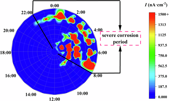
Corrosion big data clock diagrams of the ACM corrosion current.
For Q235 steel, the data indicates a distinct period of heightened corrosion activity, primarily occurring between 10:00 PM on the first day and 10:00 AM the following morning. This timeframe corresponds to the nighttime and early morning hours in Guangzhou, during which low temperatures and high humidity promote condensation. The resulting thin liquid film on the steel surface creates an electrochemical environment that accelerates the corrosion process30.
The clock diagram highlights specific timeframes of significant corrosion activity, providing an intuitive visualization of periods when corrosion is most severe. These insights are invaluable for identifying time-series data with prominent characteristics, facilitating a more targeted analysis of environmental factors and corrosion mechanisms. This focused approach enhances data interpretation, ensuring that critical periods of corrosion are effectively addressed in both research and practical applications.
Although the clock diagram intuitively shows the real-time corrosion process of Q235 steel, quantitatively analyzing the extent of corrosion remains challenging. The integral of the relative current intensity over time provides a measure of the cumulative total corrosion, as represented by Eq. (1).
Where ({Q}_{i}) represents the cumulative corrosion amount detected by the corrosion sensor, measured in coulombs (C). In is the relative corrosion current intensity at time (n=t), and ∆t is the time interval, set to one hour. Each time the relative corrosion current intensity is recorded, Qi is cumulatively calculated and plotted as a cumulative corrosion curve.
Figure 3 illustrates a sharp increase in the cumulative corrosion electric quantity (Q) of Q235 steel over a 30-day period. As time progresses, corrosion products accumulate on the steel surface, with the deepening color reflecting the advancement of corrosion. During the rapid increases in cumulative corrosion charge observed in stages 1–2 and 3–4, the number of localized corrosion spots on the surface rises significantly, accompanied by the increased presence of yellow corrosion products. This indicates a strong correlation between the cumulative corrosion electric quantity and the material’s surface morphology.
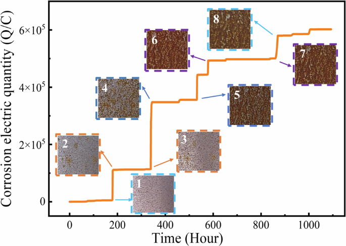
Cumulative corrosion current and macroscopic morphology diagram.
The surge in cumulative corrosion electric quantity during stages 1–4 of Fig. 3 is significantly greater than that observed in stages 5–8. The rapid increase in the early stages is attributed to oxidation reactions between the Q235 steel surface and atmospheric oxygen and humidity, resulting in the formation of iron oxides. In the later stages, the rate of increase in corrosion electric quantity gradually slows as a denser oxide layer forms on the steel surface. These corrosion products progressively cover the substrate, reducing its interaction with the environment, thereby mitigating corrosion and stabilizing the cumulative charge accumulation.
The step-like rises observed in the cumulative charge curve during this one-month observation period are notable. These abrupt changes reflect the dynamic corrosion behavior in the early stages, where environmental factors such as humidity and oxygen exposure play a significant role in the formation and evolution of iron oxides. Over longer periods, the cumulative corrosion charge would likely result in a more gradual increase in the curve, as the corrosion process stabilizes with the development of protective oxide layers. Extending the observation period could provide a more comprehensive view of the cumulative charge behavior, likely smoothing the curve and reducing the apparent sharp fluctuations.
Image preprocessing results and analysis
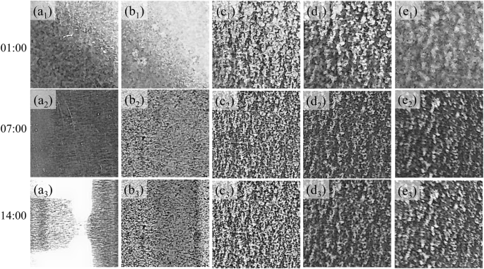
We selected corrosion images captured at 01:00, 07:00, and 14:00 on the 1st, 7th, 14th, 21st, and 35th days of the corrosion test, as shown in Fig. 4. On the first day of the experiment, the metal surface was shiny and showed no signs of corrosion. Over time, corrosion spots began to appear, with their density increasing and clustering in certain areas, making the corrosion more evident. In the later stages, the corrosion area expanded significantly, eventually covering the entire Q235 steel surface and indicating severe damage. Due to the angle of sunlight and the influence of the camera flash, the corrosion condition in some images, such as Fig. 4a3 at 14:00 and Fig. 4e1 at 01:00, was not clearly visible.
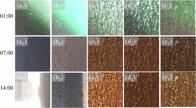
a1–a3 Day 1, b1–b3 Day 7, c1–c3 Day 14, d1–d3 Day 21, e1–e3 Day 35.
Figure 5 illustrates that the grayscale image after CLAHE processing, where corrosion spots and surface textures become more distinct, especially in the late stages (Fig. 5c–e). This leads to a clearer visualization of corrosion distribution and density. The CLAHE algorithm enhances contrast and surface detail by equalizing brightness and reducing lighting effects, thereby making even the initial stages (Fig. 5a, b) more visible.
a1–a3 Day 1, b1–b3 Day 7, c1–c3 Day 14, d1–d3 Day 21, e1–e3 Day 35.
To assess the effectiveness of CLAHE, we compared the pixel histograms of images before and after processing, as shown in Fig. 6. The original image’s histogram (Fig. 6a, b) reveals concentrated pixel intensities between 100 and 150, indicating limited dynamic range and potential detail loss. The CLAHE algorithm addresses this issue by evenly distributing pixel intensities across a broader range (Fig. 6c), enhancing both dark and bright regions, while controlling noise and improving overall image quality.
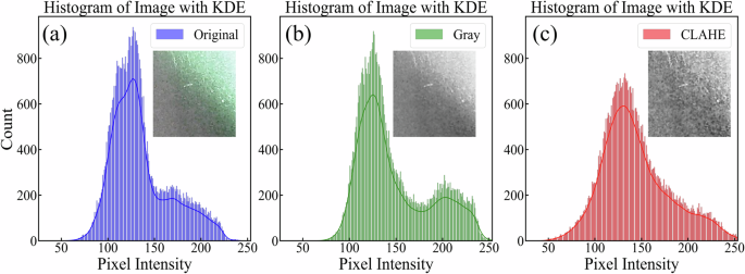
a Pixel intensity histogram of the original image, b pixel intensity histogram of the grayscale image, c pixel intensity histogram of the image processed by the CLAHE algorithm.
In terms of feature extraction, Fig. 7 illustrates that CLAHE algorithm significantly improves texture and contrast in GLCM analysis. The original image (Fig. 7a) exhibits lower contrast (572.10), while the CLAHE-processed image (Fig. 7c) achieves higher contrast (618.06), leading to sharper texture differentiation and a more compact structure. This demonstrates CLAHE’s effectiveness in both improving image contrast and enhancing texture analysis.
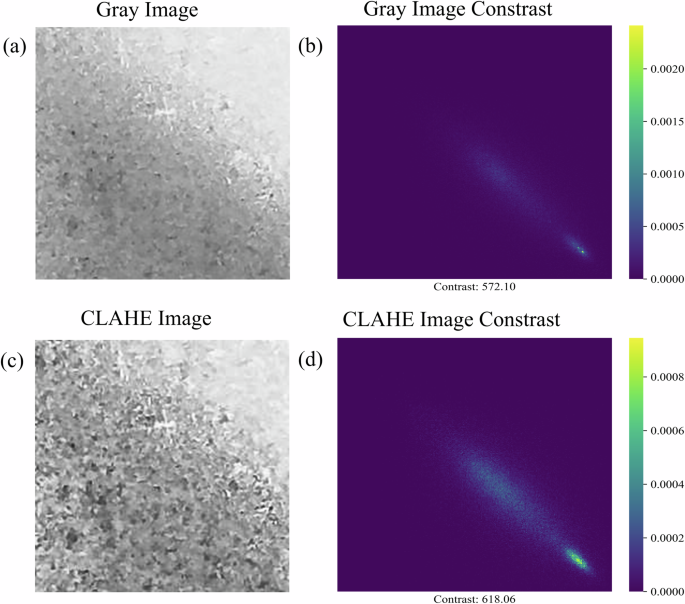
a Local details of the grayscale image, b visualization of GLCM features for the original image, c local details of the image after CLAHE processing, d visualization of GLCM features for the CLAHE-processed image.
To evaluate the impact of the CLAHE algorithm on the correlation between image features and corrosion electric quantity (Q), Spearman correlation coefficients31 were calculated for each feature before and after processing. Figure 8 illustrates that CLAHE significantly increased correlations across multiple features. By comparing the heatmaps in Fig. 8a (after CLAHE) and Fig. 8b (before CLAHE), the coefficients for LBPuniform3 and Contrast increased from 0.53 to 0.65 and from −0.70 to −0.91, respectively. These enhancements indicate that CLAHE not only improves visual clarity but also strengthens the statistical relationships between image features and the corrosion process, thereby providing a more robust framework for analyzing corrosion-related phenomena.
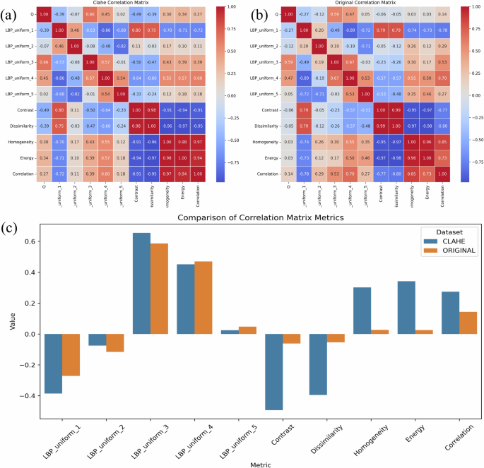
a Correlation coefficient matrix of data after CLAHE processing, b correlation coefficient matrix of original data, c comparison of correlation metrics between CLAHE-processed data and original data.
Figure 8c further highlights the improvements in feature metrics following the application of CLAHE. Specifically, the correlation between contrast and corrosion metrics increased by 30%, while homogeneity also exhibited a significant enhancement. These results confirm CLAHE’s effectiveness in strengthening the relationship between image features and corrosion metrics, thereby facilitating more robust quantitative analysis.
The effectiveness of the CLAHE algorithm in improving feature extraction has been demonstrated in the dataset used in this study. To further evaluate its performance across different materials and imaging settings, we applied CLAHE to five common metal surface images. We then calculated the GLCM features and pixel histograms for both the original and CLAHE-processed images. The results are shown in Fig. 9.
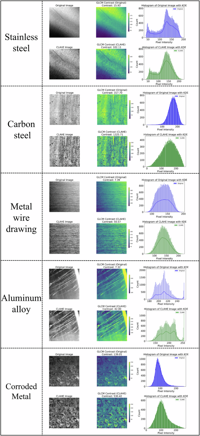
Comparison of CLAHE performance on the surface images of different metal materials.
As Fig. 9 shows, CLAHE significantly enhances contrast and detail for complex textures and rough surfaces, such as carbon steel and corroded metal. For example, the GLCM contrast for carbon steel increased from 317.70 to 1325.71, and for corroded metal from 139.01 to 530.42. Additionally, histograms became more uniform, improving detail visibility. However, the enhancement effect is more limited for smooth, highly reflective materials such as aluminum alloy and brushed metal surfaces. For instance, the GLCM contrast for aluminum alloy only increased from 7.32 to 42.00, suggesting that CLAHE’s effectiveness is influenced by the surface characteristics of the material.
Moreover, different imaging settings can significantly affect the processing results. Overall, the CLAHE method is well-suited for enhancing complex surface features and corrosion analysis, but for regular textures and smooth surfaces, it should be combined with other enhancement techniques for optimal results.
Atmospheric corrosion evaluation model
To address the limitations of traditional Q235 steel corrosion detection methods, this work introduces Qcorr, a linear atmospheric corrosion evaluation model. Traditional approaches, such as weight loss techniques and electrochemical measurements, suffer from long detection cycles, poor real-time capabilities, and high equipment requirements. Qcorr overcomes these challenges by integrating image-based features and environmental parameters to provide a rapid and accurate assessment of corrosion levels in Q235 steel. This innovative approach offers a streamlined solution for real-time corrosion monitoring in variable conditions.
To identify the most critical features influencing Q235 steel corrosion from the dataset, we applied the extra trees model to evaluate feature importance. The extra trees model excels in handling high-dimensional data and capturing nonlinear relationships, making it highly effective for feature selection32. The evaluation results from this model are shown in Fig. 10.
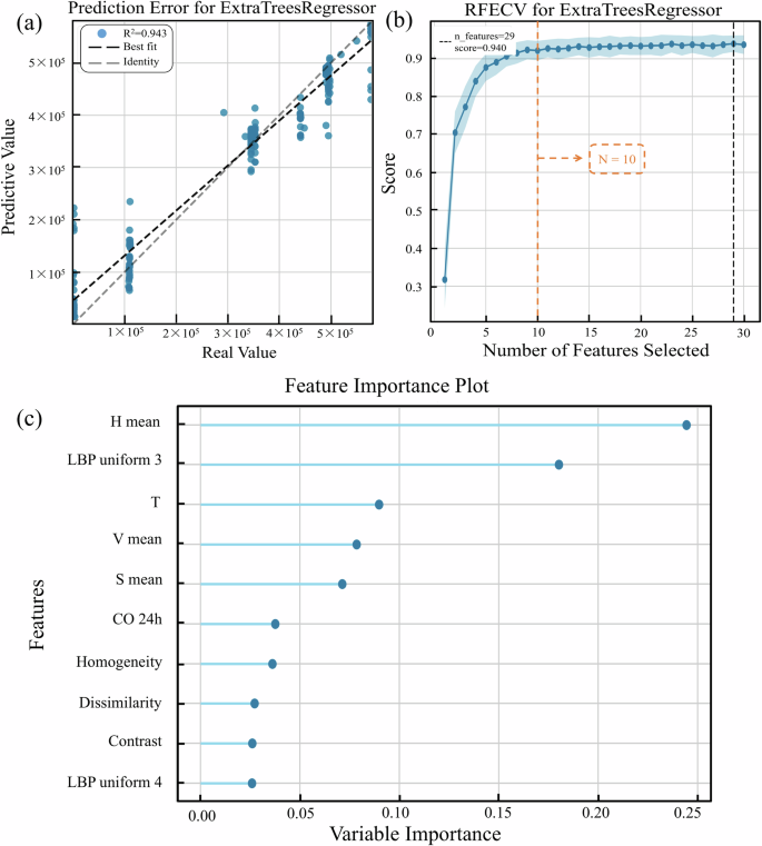
a Prediction error plot, b learning curve, c feature importance plot.
From Fig. 10a, we observe that most data points lie close to the fit line, with an R2 value of 0.943 on the test set, demonstrating the model’s strong fit. The learning curve in Fig. 10b shows that the model’s accuracy increases rapidly as more features are selected, stabilizing when the top 10 features are included. Based on this, we selected the top 10 key features for the model construction process, as shown in Fig. 10c. These features include image texture and color characteristics, along with environmental data, all of which play a crucial role in predicting the corrosion degree of Q235 steel.
Based on the selected key features, the following linear model, Qcorr, has been constructed as shown in Eq. (2):
Where β is a constant with a value of −1,454, 119.07. When i range from 1 to 3, it represents the color features of the image, specifically the mean values of the H, S, and V channels. When i range from 4 to 5, it corresponds to the image’s LBP features. From 6 to 8, i represents the GLCM features of the image. Finally, when i range from 9 to 10, it refers to environmental features. The specific feature values are listed in Table 1 under image and environmental features.
This linear model utilizes key features to accurately predict the cumulative corrosion electric quantity (Q), facilitating real-time monitoring of the Q235 steel corrosion process. To assess the model’s performance, Fig. 11 shows the evaluation results, including the model’s accuracy and prediction capabilities.
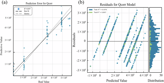
a Model prediction error, b model residual plot.
Figure 11a shows that the linear model achieves an R2 value of 0.897, indicating strong predictive performance. Figure 11b confirms that the model performs similarly on both training and testing datasets, with residuals that are normally distributed and centered around zero. This consistency validates the reliability of the Qcorr formula. By incorporating multi-source data, including image features and environmental factors, the model captures the complex influences of corrosion, effectively monitors surface changes, and quantifies corrosion-induced electrical signals—outperforming traditional methods. However, addressing data sparsity by expanding the dataset could further improve the model’s robustness and applicability to diverse conditions.
To evaluate the generalization and robustness of the Qcorr model, this study introduces a new image dataset as a validation set. The dataset contains 120 photographed images of carbon steel corrosion along with corresponding sensor data. An example of the image dataset is shown in Fig. 12, including the original image, the image in the HSV color space, the grayscale image, and the image processed with CLAHE.
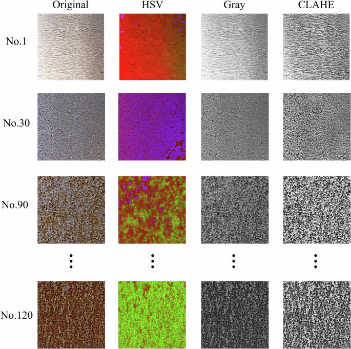
Example images from the validation dataset.
During the model validation process, the validation data is directly input into the Qcorr model for prediction, and the model’s performance is evaluated using several metrics. Figure 13 presents key performance visualizations of the model on the test dataset, including a comparison of actual vs. predicted values, residual analysis, and their distribution characteristics.
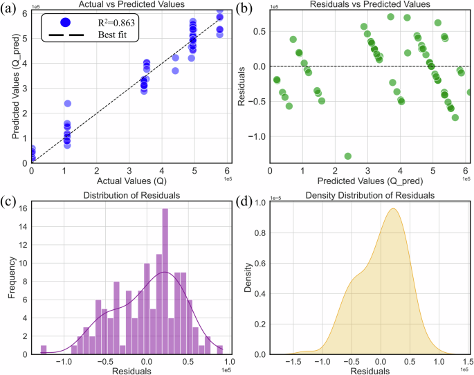
a Model prediction error, b model residual plot, c distribution of residuals, d density distribution of residuals.
Figure 13 shows the performance metrics of the Qcorr model on the validation dataset, including prediction error, residuals, and their distribution. In Fig. 13a, the model achieves an R2 value of 0.86, with most data points closely following the diagonal, indicating a strong fit despite minor deviations. In Fig. 13b, the residuals are tightly clustered around zero, showing minimal systematic bias, though larger residuals may occur due to local anomalies or feature limitations. Figure 13c shows a nearly normal distribution of residuals, with a longer right tail compared to the left, indicating occasional overestimations by the model. Finally, compared to Fig. 13b, Fig. 13d offers a clearer view of residuals tightly clustered around zero, further emphasizing the model’s stable predictive performance.
In summary, the Qcorr model demonstrates high accuracy during training and validation, highlighting its potential as a reliable tool for monitoring and analyzing the corrosion process of Q235. While its predictive performance is suboptimal in certain intervals, the model’s simplicity and strong interpretability enable rapid iteration and improvement. Expanding the diversity of the training data can enhance the model’s generalization and adaptability to a wider range of environments, further strengthening its performance under varied operating conditions.
Methods
Outdoor exposure data collection
The outdoor exposure test was conducted at the National Environmental Corrosion Platform (NECP) standard exposure test site in Guangzhou, Guangdong province, China. The experiment adhered to the ISO9226-2012 standard to ensure both data reliability and standardization. Figure 14a presents an overview of the test site. The experimental configuration included a corrosion sensor, temperature and humidity sensors, environmental sensors, an image collector, and a standard Q235 steel corrosion specimen (100 × 50 × 5 mm). A CCD camera was positioned 50 cm in front of the specimen for image acquisition (Fig. 14b). Figure 14c illustrates the configuration of the corrosion sensor, which comprises a Q235 steel working electrode and copper sheets functioning as the reference and counter electrodes. These components are separated by a 0.1 mm glass-fiber reinforced epoxy resin layer, effectively preventing direct contact between the anode and cathode. Both electrodes have an exposed area of 21 × 21 mm2. The sensor assembly was encased in epoxy resin, and its surface was polished with 1200-grit sandpaper to ensure smoothness and accurate data acquisition.
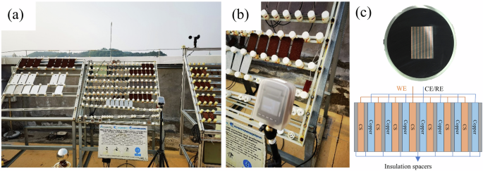
a Full view of the outdoor exposure test site, b image acquisition device, c corrosion sensor.
The data acquisition process lasted 46 days, with the corrosion sensor and environmental data sensor collecting data every minute, and the CCD camera every hour. During this period, corrosion sensor, environmental sensor, and camera data were timestamped to align the data and ensure consistency and accuracy across the multiple sources. Finally, corrosion sensor data, environmental data, and corrosion images were acquired.
Image processing and analysis
In this study, image preprocessing and analysis techniques were applied to enhance the detection of corrosion on Q235 steel surfaces under varying environmental conditions.
Image preprocessing
In computer graphics, a 224 × 224 pixel input image is commonly used to preserve essential features and details across diverse scenes and object types. This resolution effectively balances the capture of both global context and local information. Prominent models such as AlexNet, VGGNet, and ResNet have successfully adopted this approach. Following this principle, we cropped the original 2048 × 1536 pixel images to 224 × 224 pixels, minimizing redundant information while emphasizing critical areas of the corroded specimens. This preprocessing step ensures data consistency and enhances the accuracy of subsequent analyses.
To address lighting inconsistencies that could impact feature extraction, the Contrast Limited Adaptive Histogram Equalization (CLAHE) algorithm was applied. CLAHE divides each image into small, non-overlapping regions, applies histogram equalization to each, and smooths the resulting histograms using a clipping operation to avoid noise amplification. These clipped histograms were used to adjust the image contrast, and the clipped value ({L}_{c}) was calculated using Eq. (3).
Where Wt and Ht represent the width and height of the sub-blocks, respectively, while Ng denotes the number of grayscale levels, and Fc is the clipping factor. Subsequently, the CLAHE algorithm normalizes each pixel using the cumulative distribution function (CDF) to compute the output pixel value, as shown in Eq. (4).
Where ({{cdf}}_{{input}}; {rm{pixel}}) represents the CDF value of the input pixel, ({{cdf}}_{{min }}) denotes the minimum CDF value among the input pixels, and ({rm{gray}}; {rm{levle}}_{{max }}) indicates the maximum grayscale level.
To ensure a smooth transition between sub-blocks, the CLAHE algorithm employs bilinear interpolation to calculate the pixel value I (x, y), as illustrated in Eq. (5).
Where (Delta x) and (Delta y) represent the pixel offsets along the x and y axes, respectively, and ({I}_{1-4}) denotes the grayscale values of the four neighboring pixels. The final output image is obtained through the above calculations.
Feature extraction
Various image analysis techniques were applied to better understand the corrosion process on Q235 steel surfaces. Since RGB (red, green, and blue) color values are prone to environmental fluctuations33, we converted the images to the more stable HSV (hue, saturation, and value) color space for analysis. The conversion equations are provided in (6) and (7).
Where MAX represents the maximum value of R, G, and B, MIN represents the minimum, and δ is defined as MAX–MIN. H, S, and V are the corresponding components of R, G, and B in the HSV color space.
The local binary pattern (LBP) and gray level co-occurrence matrix (GLCM) algorithms were employed to extract texture features from the HSV images. For the LBP analysis, we implemented the uniform pattern method proposed by Ojala et al.34. The image was converted to grayscale, and the LBP algorithm was applied with a radius of 1 and 8 sampling points. This process involved comparing the center pixel to its 8 neighbors within a 3 × 3 window to generate 8-bit binary sequences.
The resulting LBP values effectively encode local texture features, with lower values representing uniform regions and higher values indicating complex patterns such as edges and corners. This approach simplifies texture analysis by capturing key spatial characteristics, including edges and flat areas.
The GLCM algorithm constructs a two-dimensional matrix that quantifies the co-occurrence relationships between different gray levels in specific spatial directions and distances. This matrix reveals the spatial distribution of pixel intensities within an image35. Specifically, the algorithm analyzes pairs of adjacent pixels, generates a co-occurrence matrix based on their gray levels, and extracts texture features such as contrast, homogeneity, energy, entropy, and correlation36,37,38. To ensure comparability across different images, the matrix values are normalized to represent relative frequencies.
Contrast measures intensity differences between neighboring pixels, with higher values indicating sharper edges and greater texture variability. Dissimilarity quantifies intensity variation but does so linearly, providing a straightforward measure of variability. Homogeneity evaluates texture uniformity, assigning higher values to smoother patterns and lower values to coarser, irregular textures. Energy reflects repetition and regularity, where higher values correspond to structured patterns, and lower values indicate randomness. Finally, correlation measures the linear dependency between pixel intensities, with higher values signifying more organized and predictable textures.
The distribution of the extracted image features is presented in Fig. 15, encompassing contrast, dissimilarity, homogeneity, energy, LBP uniform patterns, and the mean values of the HSV color components. The figure highlights distinct distribution patterns for each feature. For example, contrast exhibits a wide, multimodal distribution, while homogeneity and energy are more concentrated, reflecting greater consistency in these features.
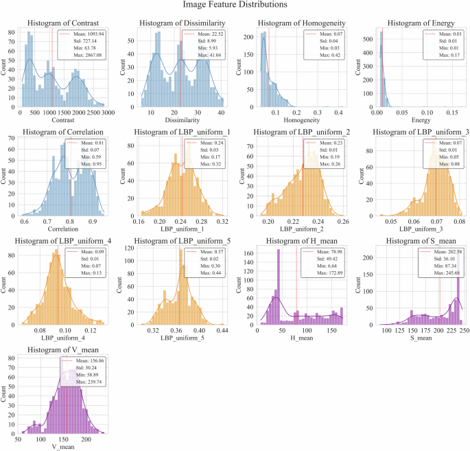
Distribution of image features.
Numerical data processing
The numerical dataset comprises corrosion sensor readings, such as corrosion current (I), temperature, and humidity, alongside environmental indicators, including PM2.5, PM10, SO2, NO2, O3, CO, and air quality index (AQI) metrics. The dataset contains only a small number of missing values. Saeipourdizaj demonstrates that the k-nearest neighbor (KNN) algorithm performs comparably to interpolation methods for handling missing environmental data39. Given the relatively stable trends observed in corrosion sensor and environmental data, linear interpolation offers a faster solution for filling missing values while effectively preserving local patterns. Consequently, we selected the piecewise linear interpolation method for addressing missing data. The linear interpolation formula is provided in Eq. (8).
Where ({x}_{i}) represent the index of a known data point, and ({y}_{i}) its corresponding function value. For a given interpolation point (x), the interval [({x}_{i},{x}_{i+1})] containing (x) is first identified. The interpolated value (y) is then calculated using the linear interpolation formula based on the known points (left({x}_{i},{y}_{i}right)) and (left({x}_{i+1},{y}_{i+1}right)).
Following pre-processing, a statistical analysis of the numerical data distributions was conducted, as depicted in Fig. 16. The distributions of key sensor features, including corrosion current (I), AQI, CO, NO2, O3, PM10, PM2.5, and SO2, are represented as histograms. The distribution patterns vary significantly across sensors. For instance, the corrosion current (I) exhibits a sparse distribution with high variance, while AQI, NO2, and PM2.5 display more concentrated, positively skewed distributions. In contrast, O3 and CO distributions are more dispersed, reflecting greater variability in these pollutants.
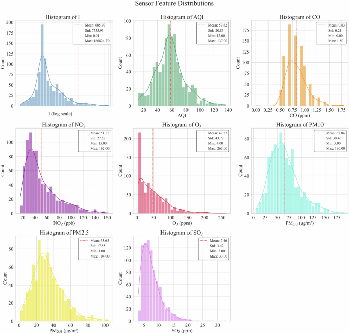
Distribution of numerical data.
Finally, the full numerical data was assembled. The LBP and GLCM features extracted from the images were then combined with the environmental data and the timestamped corrosion sensor data, as shown in Fig. 17. This integration formed the final dataset for modeling and analysis.
Fusion process diagram of corrosion sensor data and image data.

Responses