Residual strength prediction of corroded pipelines based on physics-informed machine learning and domain generalization

Pipelines are crucial for the transportation of oil and gas resources. Due to the poor service environment, pipeline corrosion degradation can frequently occur^1,2, which can lead to the material deterioration and leakage failure, resulting in financial losses and environmental pollution. Residual strength can properly reflect the pressure limit of in-service pipelines^3,4, which is an important indicator for pipeline reliability assessment. Therefore, in order to ensure the transportation safety and pipeline integrity, an accurate residual strength prediction model is necessary.

At present, numerous studies have been conducted for residual strength prediction of corroded pipelines. The empirical formulas, finite element method (FEM), and machine learning (ML) models are the most commonly used approaches⁵. The empirical formula has attracted much attention due to its simple calculation, which is established by researchers based on fracture mechanics and pipeline burst experiment. The formula NG-18 was obtained by Battelle Research Institute in the United States based on fracture mechanics and blasting experiment⁶. The American Society of Mechanical Engineers (ASME) proposed the ASME B31G standard and made improvements on this basis^7,8. In order to improve the calculation accuracy of this method, Modified ASME B31G was used to revise the expression of failure stress⁹. DET Norske Veritas and British Gas Company proposed the DNV-RP-F101 through a large number of burst experiments¹⁰, which improves the accuracy and simplifies calculation process. Battle laboratory proposed the PCORRC standard based on FEM analysis¹¹, and it used ultimate strength instead of flow stress. These empirical formulas have wide application in engineering practice due to their high computational efficiency. However, the empirical formulas are relatively conservative, and the predicted values are usually lower than actual values, which may cause unnecessary economic losses. In addition, the empirical formulas cannot be applied to pipeline steels of all strengths¹², the generalization performance is poor.

In practical engineering, the corrosion defects of pipelines are not isolated and single^13,14,15. Multiple defects may lead to the interaction between defects, which makes the prediction of residual strength more complicated. The FEM utilizes computer technology to simulate the pipeline conditions to predict the residual strength of corroded pipelines. Residual strength refers to the ultimate bearing capacity of defective pipelines, typically expressed in terms of burst pressure. Huang et al.¹⁶ developed a FEM-based model to predict the failure pressure of pipelines containing a dent-corrosion defect, the results demonstrated that the dents could reduce the failure pressure. Chen et al.¹⁷ used the FE method for residual strength prediction of subsea pipelines with asymmetrical corrosion defects. Gholami et al.¹⁸ applied a semi-empirical technique for predicting the residual strength of defective pipelines, and FEM simulation was used to assess the impacts of influence factors on the residual strength. Kere et al.¹⁹ developed a probabilistic model with correction factor to predict the burst failure pressure of thin-walled pipelines with single crack-like defect, the XFEM was conducted to obtain the numerical data. Shuai et al.²⁰ established a nonlinear FEM model to predict the failure pressure of corroded pipelines subjected to external loads. The effects of bending moment and axial force on the burst capacity were investigated. Mensah et al.²¹ proposed a novel burst pressure prediction model for corroded pipelines with interacting corrosion clusters, the numerical models established by FEM and improved composite defect shapes are proposed to improve the prediction accuracy. Although accurate prediction results can be obtained by FEM, the expensive time cost and computational burden have restricted the computational efficiency. In addition, the modifications of FEM model are required when the parameters of pipelines and defects are changed, which makes it difficult to achieve rapid assessment for residual strength.

In recent years, ML models have received attention for residual strength prediction of corroded pipelines, due to their proficiency in capturing intricate relationships. Phan et al.²² utilized the adaptive neuro fuzzy inference system (ANFIS) and principal component analysis (PCA) for evaluating the burst pressure of defective pipelines. Abyani et al.²³ proposed an efficient FEM model and several ML models for failure pressure prediction of corroded offshore pipelines, which could improve the computational efficiency. Xiao et al.¹² used the several interpretable ML models for predicting the failure pressure of corroded pipelines, the physical factors related to pipeline failure mechanisms are integrated, and the SHAP method is utilized to improve the model interpretability. Li et al.²⁴ developed a data-driven method for residual strength prediction of subsea pipelines with double corrosion defects, the Bayesian regularized artificial neural network (BRANN) was used based on the dataset generated by FEM. Phan et al.²⁵ established a data-driven approach for burst pressure prediction based on various ML models, which achieves a significant improvement of prediction accuracy. Ma et al.²⁶ established a novel hybrid model for predicting the burst pressure, which combines empirical formula and ensemble learning, it can make full use of prior knowledge. Chen et al.²⁷ utilized the multi-layer perceptron (MLP) with dropout method for residual strength prediction, which can solve the problem of inadequate training data. Miao et al.²⁸ built a novel residual strength prediction model based on based on deep extreme learning machine (DELM). The hybrid teaching-learning-based optimization (HTLBO) algorithm was designed to improve the prediction accuracy. Taiwo et al.²⁹ provided a systematic review of modeling the failure probability of water pipes, including physical, statistical, and ML models, failure probability integration methods are also discussed. El Amine Ben Seghier et al.³⁰ examined eight ML models for failure mode identification of corroded pipelines, and Shapley additive explanations approach is utilized to explain the ML model.

Although the extensive research has delved into residual strength prediction of corroded pipelines using ML techniques, however, there are still some limitations:

• Considering the opaque “black-box” system of present ML models^31,32, physical prior knowledge has been incorporated into ML models, and feature selection is performed based on the correlation analysis for improving the prediction performance. However, the feature number, prediction accuracy and model stability are all important for feature selection, which has not yet been comprehensively considered.

• In practical engineering, many factors can affect the residual strength of corroded pipelines, such as external loads, multiple defects, etc. Nevertheless, the present dataset is related to the working condition of single defect, and it is impossible to collect data under all application scenarios, so there is a notable gap in evaluating the applicability of ML models, the model generalization needs to be improved.

• ML models optimized by intelligent optimization algorithms have been frequently employed, but these algorithms are short of self-exploration mechanism and add much computational burden, which may restrict the improvement of prediction accuracy and computational efficiency.

Motivated by the above research gaps, this paper proposes a novel physics-informed domain generalization model for residual strength prediction of corroded pipelines. The main contributions of this paper are as follows:

• A physics-informed feature space containing original features and new features with physical meaning is constructed.

• The feature importance of all feature variables is evaluated to improve the model interpretability, and several feature subsets with different feature combinations are established. Feature selection is conducted considering the multi-objective factors, namely prediction accuracy, model stability and feature number.

• Based on the new feature space, a novel physics-informed domain generalization model is proposed for residual strength prediction. a deep forest (DF) model coupled with double deep Q-network (DDQN) is firstly developed to improve the self-exploration capacity and ensure the prediction performance.

• A comprehensive dataset of corroded full-scale pipelines is collected for model validation, and domain generalization performance is verified for different application scenarios, including external loads and multiple defects.

The results of feature selection

The feature importance is calculated using the Gini coefficient. The larger the value of feature importance, the more information the feature contains. Figure 1 shows the importance ranking of the input features. In the physics-informed feature space, the defect length l is of greatest importance, followed by l²/D(t–d), l²/Dt, d. It can be indicated that the features related to defect length and defect depth are more important than other features.

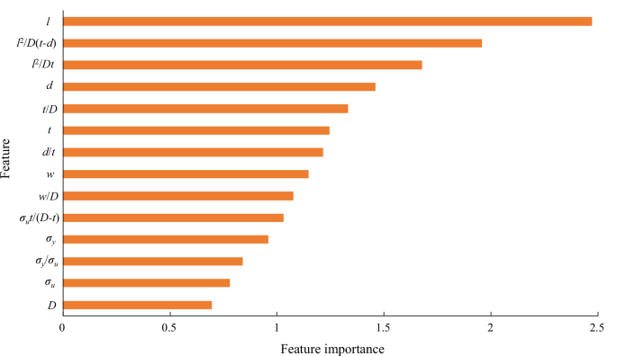
The results of feature importance.

Full size image

It is necessary to select the most suitable feature subset based on the order of feature importance, and the feature variables that have greater importance are prioritized for selection. However, an excessive number of features can increase the computational cost, while a small number of features can result in information omission.

In order to achieve desired high prediction performance and computational efficiency at the same time, feature selection is performed to select the optimal feature subset that consists of a part of input features. Therefore, this study presents an evaluation indicator considering prediction accuracy, model stability and feature number comprehensively, as shown in Eqs. (1)–(2). The ratio of optimal feature subset and total feature numbers represents the computational cost.

where μ is the ratio of feature number of feature subset and total feature number; d is the feature number of feature subset; m is the total feature number; (overline{mu }),(overline{MAPE}) and (overline{STD}) are corresponding values after normalization; w₁, w₂ and w₃ are the weight coefficients, the values are as follows³³: w₁ = 0.2, w₂ = 0.4, w₃ = 0.4.

The feature subset is selected with priority to more important features. The comprehensive evaluating indicator C in Eq. (1) is utilized to select the optimal feature subset. The smaller the value of C, the better the comprehensive performance of model. Table 1 shows the results of comprehensive evaluating indicator for different feature subsets. D_i (i = 1, 2, …, 14) represents the feature subset that contains the first i important input features. Each feature subset is input into the proposed physics-informed model. After calculation, D₈ is determined as the optimal feature subset for model input, which can simultaneously improve the prediction performance and reduce the computational cost.

The prediction results of proposed model

The mean square error (MSE), mean absolute error (MAE), MAPE, R², and STD are selected to evaluate the prediction performance, as shown in Eqs. (3)–(7). For these evaluation metrics, the closer the value of R² is to 1, the more efficient the model is. For MSE, MAE and MAPE, the lower the values of these evaluation metrics, the more accurate the model is. Also, the lower the STD, the better the model stability is.

where ŷ_i and y_i are the predicted and actual values of burst pressure respectively; ӯ is the average value of actual burst pressure; n is the number of samples.

After constructing the environment of deep reinforcement learning, the action space contains 12 actions. The capacity of experience pool is 100, the learning rate α is 0.001, and the discount factor γ is 0.99. The greediness ε is set to 0.9, which means the probability of selecting the action with the maximum Q value is 90%, and the probability of randomly selecting actions is 10%. The results of DF model coupled with DDQN and DQN for testing dataset are shown in Table 2. As can be seen from Table 3, for the DF model coupled with DDQN, MSE is 2.113, MAE is 0.913, MAPE is 6.158%, R² is 0.951, STD is 1.401. Compared with the final prediction results of DQN, the DF model coupled with DDQN has higher prediction accuracy and model stability.

In order to verify the effectiveness of new feature space, the model with the input of original features is compared with the physics-informed model. Figure 2 displays the prediction results of the models with the input of the optimal feature subset D₈ and original features (no physical information). To avoid other factors affecting the prediction results, the proposed model is both used for different input features. It can be seen that the prediction accuracy of the proposed model with hybrid features is better than that with original features, which indicates the effectiveness of physics-informed feature space.

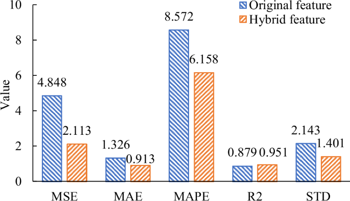
The prediction results of the models with the input of hybrid features and original features.

Full size image

The results of domain generalization

In order to verify the domain generalization performance, the application scenarios of external loads and multiple defects are introduced. The axial compression force (F) and bending moment (M) can influence the pipeline residual strength. Three groups of data for corroded pipelines with external loads are shown in Table 3³⁴. Figure 3 shows the prediction results of different models. It can be seen that the proposed model performs better in residual strength prediction under external loads than empirical formulas, the maximum relative error is 9.5%, which indicates that the proposed physics-informed model can achieve the domain generalization for external loads.

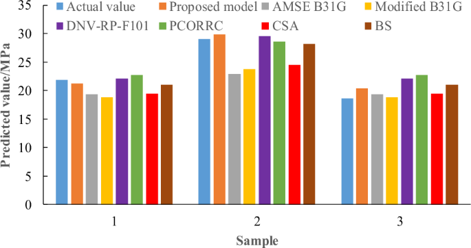
The prediction results of different models for corroded pipelines with external loads.

Full size image

The interaction between multiple corrosion defects can lead to the complex stress conditions. When the distance between two corrosion defects is small enough to a certain extent, the residual strength will be additionally weakened due to the connectivity of high-stress areas, as shown in Fig. 4. The collected data of multiple corrosion defects is shown in Table 4^24,35. The effective length and effective width are the sum of interval and defects’ length and width. The effective depth is the maximum corrosion depth of multiple defects.

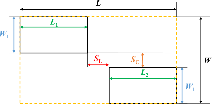
The schematic diagram of two corrosion defects.

Full size image

Figure 5 shows the prediction results of different models for multiple corrosion defects. It can be seen that the proposed model presents the best prediction performance compared to empirical formulas, and the maximum relative error and average relative error are 9.67% and 4.86%, respectively. The PCORRC also performs well in some samples for residual strength prediction, but the average relative error is 6.4%. Therefore, the proposed physics-informed model can achieve the domain generalization for the working condition of multiple corrosion defects.

The prediction results of different models for multiple corrosion defects.

Full size image

The prediction results of different models for different steel grades

The prediction models may have different prediction results for different pipeline steel grades. This paper validates the generalization performance of the proposed model and empirical formulas with the dataset of low, medium and high strength pipelines. Figure 6 shows the prediction results of different models for different pipeline steel grades. The material grades that are <X60 are set as low strength steels. X60, X65 and X70 are medium strength steels. X80 and X100 are high strength steels. Total represents the overall combination of low, medium and high strength pipelines. It can be clearly seen that the proposed model has the best prediction performance for all grades of pipeline steel. For total dataset, PCORRC has the highest prediction accuracy in several empirical formulas. Among low strength steels, PCORRC is also the most suitable model. Among medium strength steels, BS is most successful for predicting the residual strength of corroded pipelines. Among high strength steels, PCORRC and CSA both have better prediction performance. Thus, for traditional empirical formulas, PCORRC has the best applicability to different pipeline steel grades. But the prediction accuracy of proposed model is much higher than that of empirical formulas regardless of pipeline steel grades. Therefore, the proposed model has the best adaptability to various grades of pipeline steels.

The prediction results of different models for different pipeline steel grades.

Full size image

In order to verify the superiority of the DF model coupled with DDQN, several common optimization algorithms are applied for comparison, such as sparrow search algorithm (SSA), PSO, GA, grey wolf algorithm (GWO). The inputs of all models are the selected feature subset D₈ of physics-informed feature space. Figures 7 and 8 show the prediction results of testing dataset of five optimization methods. The base models are all selected as DF model. Like the proposed model, the optimization variables of DF model are the N₁, M and N₂. And the MSE is used as the fitness function of other four single-objective optimization algorithms. It can be seen that these five optimized models can successfully predict the residual strength, and the points of five models are all around the oblique line. But after comparison, the points of GA-DF are more dispersed than other models, and the points of proposed model are more concentrated around the slash. It means that the prediction values are in good agreement with the actual values.

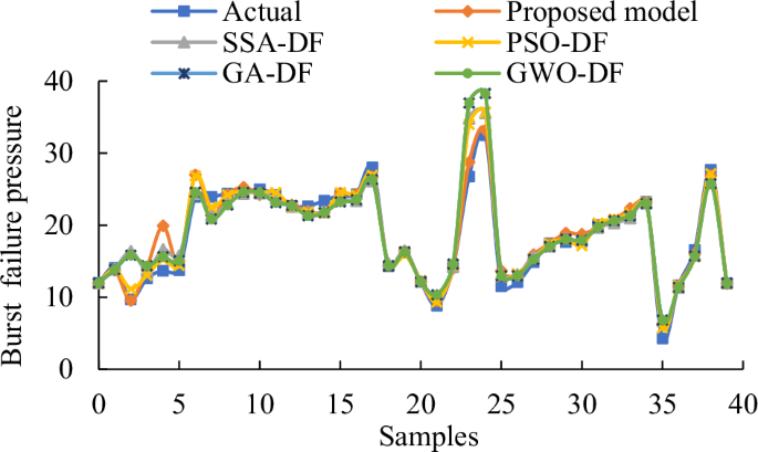
The prediction results of pipeline residual strength.

Full size image

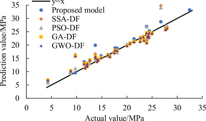
The results of correlation regression of pipeline residual strength.

Full size image

To further quantify the prediction accuracy of the five different optimization methods, Table 5 depicts the results of evaluating indicator. It can be clearly seen that the five models all achieve accurate prediction results. The values of R² are all >0.85, and the values of MAPE are all <9%. Among these models, the proposed DF model coupled with DDQN is the best in prediction results of testing dataset. The PSO-DF model also has good prediction performance in residual strength prediction. The prediction accuracy of GA-DF model is the worst, which indicates that traditional methods may easily lead to the local optimum. In addition, in terms of model stability, the proposed model also has the best performance. Consequently, the proposed model has better prediction accuracy and stability, DDQN is effective for improving the prediction performance.

The training time of different models is shown in Fig. 9, and the training epochs of these five models are all 200. It can be seen that the training time of DDQN is the shortest, and other optimization algorithms are much slower than DDQN. Although the PSO can perform well in prediction accuracy, the efficiency is the worst. Totally, the proposed DF model coupled with DDQN is more accurate and efficient than other optimization methods, which demonstrates the effectiveness of this reinforcement learning method. It is indicated that the self-learning method is advantageous in global search for the optimal hyper-parameters of DF model, which can also improve the optimization performance and computational efficiency compared to traditional optimization algorithms.

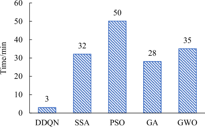
The training time of different models.

Full size image

In order to further verify the superiority of proposed model, several common ML methods are used for comparison. The RF model³⁶, BP neural network³⁷, SVR³⁸, gradient boosting regression tree (GBRT)³⁹, and extreme gradient boosting (XGBoost)⁴⁰ have been proven excellent in previous studies, so this study compares them with proposed model. The BP neural network consists of one input layer, several hidden layers and one output layer. The number of hidden layers, the number of neurons and learning rate are chosen as the optimization variables. The penalty coefficient C, allowable error ε, and kernel function coefficient γ_s are the optimization variables of SVR. For RF, GBRT and XGBoost, the number of decision trees, the maximum number of features, and the maximum depth of the decision trees are used as optimization variables. For all different ML models, the selected feature subset D₈ of physics-informed feature space is the model input.

Figure 10 and Table 6 depict the prediction results of other ML models. It can be clearly indicated that the proposed model has the best prediction accuracy among all models. The hybrid models with XGBoost, BP and RF have also achieved higher prediction accuracy, the values of R² are >0.9, and the values of MAPE are all <9%. For hybrid models, the models evolved from BP neural network have higher prediction accuracy than the models evolved from SVR. Through comparison, the hybrid ML models perform better than traditional single models. Among all models, the prediction performance of traditional BP neural network is the worst. Furthermore, the proposed model has the smallest STD, which indicates the best model stability. The results demonstrate that the proposed model has greater prediction performance than other ML models.

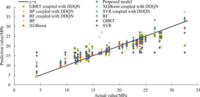
The prediction results of pipeline residual strength of other ML models.

Full size image

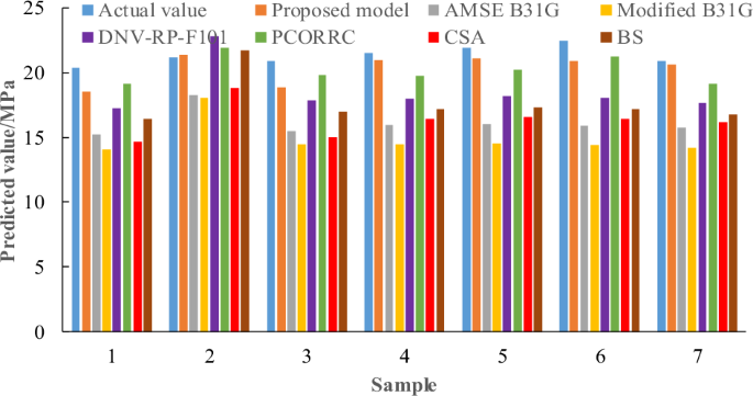
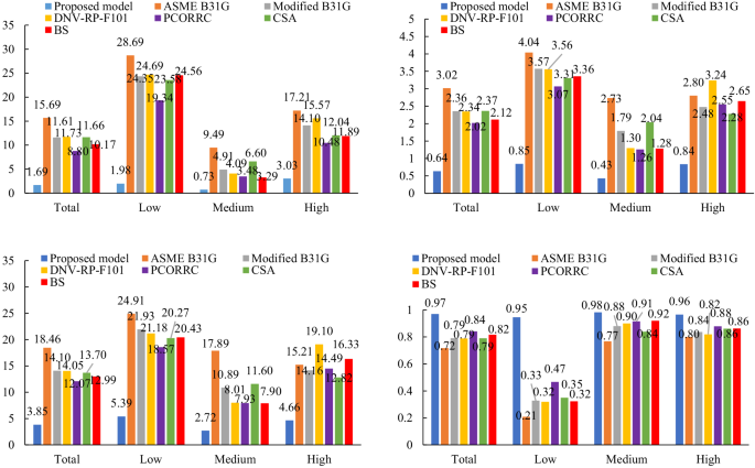
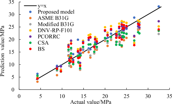
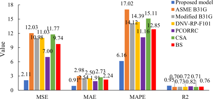
Due to the superiority in calculation speed of traditional empirical formulas, the ASME-B31G, Modified B31G, DNV RP-F101, PCORRC, CSA Z662⁴¹ and BS 7910⁴² are used to compare with the proposed model. Figures 11 and 12 display the prediction results of testing dataset of different models. Figure 11 shows that the points of traditional empirical formulas are more dispersed than the points of proposed model. For certain samples, the Modified B31G, DNV RP-F101, PCORRC and CSA models have high prediction accuracy. But for a lot of samples, these models are poor compared with proposed model. Figure 12 further shows that the results of four evaluating indicators. It can be indicated that the MSE, MAE and MAPE of proposed model are much smaller than traditional empirical formulas, and the R² of proposed model is much larger than them. Therefore, the proposed model performs better in residual strength prediction of corroded pipelines than traditional empirical formulas.

The prediction results of testing dataset of different models.

Full size image

The results of four evaluating indicators of different models.

Full size image

In summary, a physics-informed domain generalization model based on ML techniques is developed for residual strength prediction of corroded pipelines. In order to make full use of physical prior knowledge, a new feature space with physical meaning is constructed based on the empirical formulas. Based on the order of importance, several feature subsets are constructed, and the optimal feature subset can be determined considering prediction accuracy, model stability and feature number simultaneously. DF coupled with DDQN is used to establish the relationship between hybrid features and residual strength. A comprehensive dataset from burst experiment and FEM simulation is collected to verify the prediction performance. The main conclusions are as follows:

1. (1)

   By calculating the feature importance, the features related to defect length and defect depth are more important than other features. The optimal feature subset is determined as the features whose importance ranks in the top 8, which ensures the prediction performance and reduces the computational cost simultaneously.

2. (2)

   The proposed physics-informed model offers superior prediction accuracy and model stability. The MAPE, STD and R2 are 6.158%, 1.401 and 0.951, respectively. In addition, the model with the input of physics-informed feature space has better prediction accuracy than that with the input of original features.

3. (3)

   Compared with other optimization methods, the proposed model presents the best prediction performance and computational efficiency. Compared with other ML models and traditional empirical formulas, the proposed model has also significantly improved the prediction performance.

4. (4)

   For corroded pipelines of different steel grades, the proposed physics-informed model shows more excellent performance than traditional empirical formulas. For the application scenarios of external loads and multiple defects, the proposed physics-informed model also presents the best prediction performance compared to empirical formulas. The results demonstrate that this model has superior domain generalization performance.

However, this study is insufficient to investigate the influence of defect shape on the. residual strength. In practical engineering, pipeline defects can be stochastic in the appearance, thus how to consider the randomness of different defects needs to be investigated in the future.

Preliminaries

Deep forest

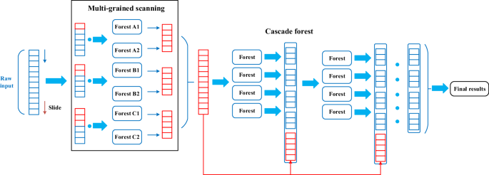
The deep forest algorithm mainly consists of multi-grained scanning and cascade forest. The multi-grained scanning uses a multiple sampling module to extract the data features⁴³. The cascade forest is a stacked structure of multiple forests, which can greatly improve the feature learning ability compared to common ensemble learning methods. In addition, compared to the deep neural network models, the hyper-parameters of DF are less, and the training efficiency is higher. Therefore, DF can provide an effective prediction for residual strength prediction of corroded pipelines.

(1) Multi-grained scanning

Multi-grained scanning is mainly inspired by convolutional neural network (CNN). Different enhanced features can be obtained by convolution kernels of different sizes. Raw data are locally multi-sampled using a sliding window for feature enhancement⁴⁴. Thus, multiple features of different dimensions are input into the cascade forest. Assuming the dimension of input sample size is S, and the dimension of sliding window is K. L represents the size of sliding step, and M represents the number of generated feature vectors. After the samples are traversed through the K-dimensional scan window, each sample subset is input into a random forest (RF) and a complete RF for training.

(2) Cascade forest

The output feature vectors of the multi-grained scanning are input into cascade forest, and the final results are output after iterative operation. It uses stacked structures to address samples layer by layer, each cascade consists of two RFs and two extreme random forests (ERF)⁴⁵. Similar to multi-grained scanning, each model in the cascade forest outputs a C-dimensional vector, so the output dimension of each layer is 4 C. The latter layer receives the feature information of the previous layer, and the output feature vectors of the previous layer are combined with the feature transformation vector P of the multi-grained scanning, which are used as the input of the next layer. The flowchart of DF is shown in Fig. 13.

The flowchart of DF model.

Full size image

Reinforcement learning

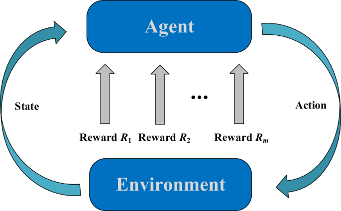
Reinforcement learning is a branch of ML methods, in which the agents can interact with the environment through a trial-and-error approach and learn the optimal strategy on the basis of the accumulated reward from previous interactions⁴⁶. It uses agents to perceive and explore the data environment, which can simulate the behavior of humans. The structure of reinforcement learning mainly includes agent, environment, state, action, and reward, as shown in Fig. 14.

The structure of reinforcement learning.

Full size image

Reinforcement learning can be divided into model-free methods and model-based methods. The model-free methods are highly flexible compared to model-based methods. Q-learning is one of the model-free reinforcement learning techniques. The learning process can be implemented during each iteration using the Q-table without prior knowledge. Deep reinforcement learning combines deep neural network and reinforcement learning⁴⁷, enabling agents to have extremely high perception and decision-making capabilities at the same time. DQN is the most commonly used method of deep reinforcement learning, and its principle is shown in Fig. 15. It integrates the neural network into Q-learning algorithm, which also belongs to model-free methods. DQN can search for optimal strategy with no need for environmental model, and the optimal strategy is determined based on the maximum cumulative reward. The prior knowledge is stored in the “experience pool”, and a certain amount of samples are extracted to train the evaluation network. Meanwhile, the target network with the same structure is introduced, and the parameters of target network are copied from evaluation network.

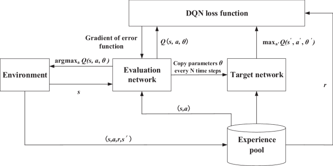
Principle diagram of DQN algorithm.

Full size image

The target Q value is calculated by the maximum of Q-value function. However, the overestimation problem of evaluated Q value may occur, leading to the super large Q value⁴⁸. DDQN model improves the calculation method of target Q, removing the parameter connection between the target Q-valued function and evaluated Q-valued function. The calculation formulas of the two methods are shown in Eqs. (8)–(9).

where t is the time; γ∈[0, 1] is the discount factor; R_t is the reward; s is the current state; a is the action; θ, θ^‘ are the parameter settings of the neural network.

In order to improve the prediction performance of ML models, the meta-heuristic algorithms are frequently used to determine the hyper-parameters with satisfactory results. However, the strategy of meta-heuristic lacks flexibility and self-exploration mechanism in the search process. In addition, some improvement on meta-heuristic algorithms is often proposed for avoiding the local optimum during optimization, which can increase the computational burden. DDQN is a method that simulates the behavior of seeking benefits and avoiding harm. Therefore, it is worth using the DDQN for optimizing the hyper-parameters of DF through self-learning, which can improve the prediction performance and computational efficiency.

Domain generalization

Domain generalization is an approach of transfer learning where the training and testing tasks are usually the same, but the data distributions in the source domains and target domains are different. Its purpose is to learn knowledge from existing source domains and generalize it to unseen target domain tasks⁴⁹, improving the model performance in different but relevant target domains. The schematic diagram of domain generalization is shown in Fig. 16. Domain generalization can eliminate the dependence on the target domain data. The source domain task is composed of multiple source domains, and the target task is based on the invisible target domains, and then the source prediction function is generalized to the unknown working condition in the target domains.

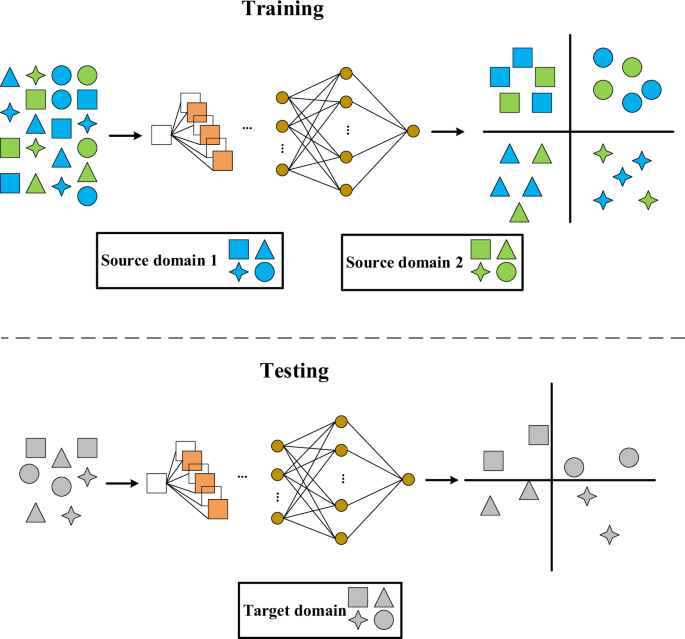
The schematic diagram of domain generalization.

Full size image

Due to the randomness of corrosion development in practical engineering, the defects may not be isolated and single. The interaction between defects can influence the pipeline safety. In addition, pipelines are mostly buried underground, so the external load can also affect the residual strength of corroded pipelines. However, it is impossible to collect the data under all working conditions from the burst experiment and FEM simulation. Therefore, it is necessary to ensure the generalization of prediction model for residual strength. The dataset of single defect collected from published literature is the available source domain, different application scenarios of external load and multiple defects are used as the target domains to verify the domain generalization performance.

Model description

The overall framework

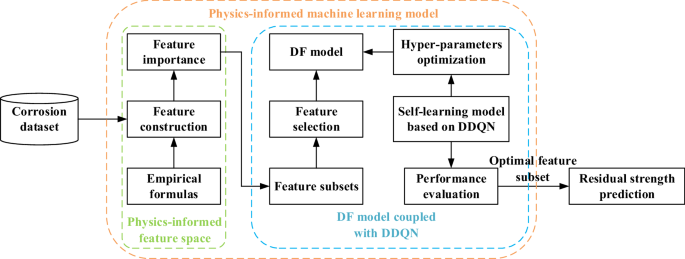
Figure 17 depicts the overall framework of the proposed model. In order to exploit the physical information, a physics-informed feature space containing original features and new features with physical meaning is constructed based on the interactive relationship between different independent variables. Feature importance is calculated using the Gini coefficient to evaluate the dependency between independent variables and residual strength. Subsequently, several feature subsets with different feature combinations are established for feature selection. The optimal feature subset can be determined comprehensively considering the prediction accuracy, model stability and feature number. Then, the DF model coupled with DDQN is proposed by introducing the self-learning parameter optimization, which can improve the self-exploration capacity and computational efficiency, and possesses significant advantages over other ML models and optimization methods. Finally, a comprehensive dataset of corroded full-scale pipelines is collected as the source domain for model validation. In order to verify the domain generalization performance, the application scenarios of corroded pipelines under external loads and multiple defects are used as the target domains.

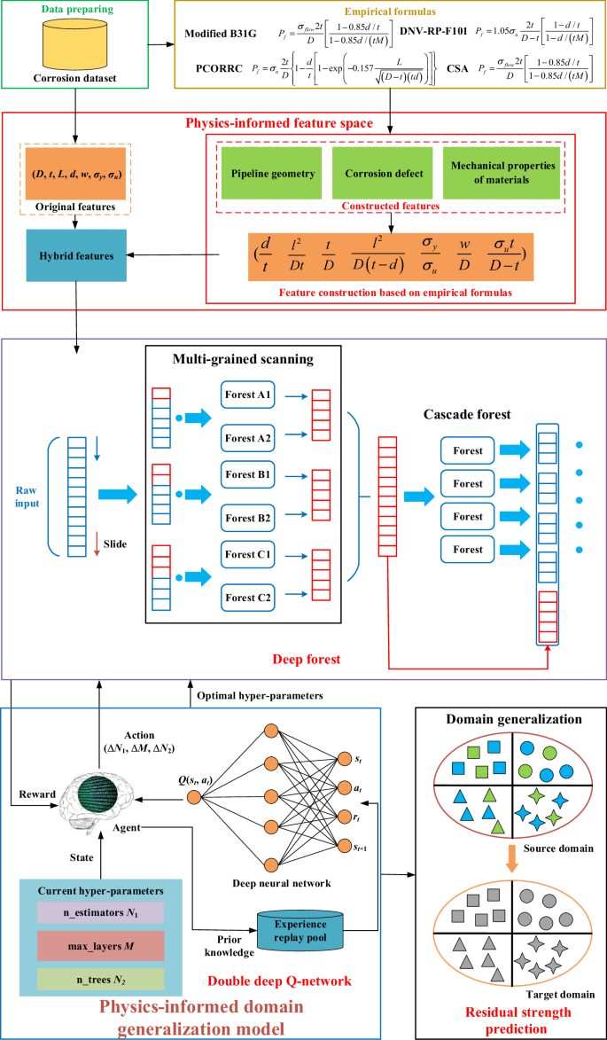
The overall framework of proposed model.

Full size image

Physics-informed feature space

Considering physical prior knowledge included in the empirical formulas, a novel feature space that incorporates physical information is constructed. In general, pipeline outer diameter D, pipeline wall thickness t, defect depth d, defect length l, defect width w, yield strength σ_y, and ultimate strength σ_u are usually used as input variables to establish the residual strength prediction model. According to the common empirical formulas in Eqs. (10)–(13), namely Modified ASME B31G⁸, PCORRC¹¹, DNV RP-F101¹⁰, and CSA Z662⁴¹, seven new features with physical meaning are constructed using feature transformation. The constructed features are d/t, l²/Dt, t/D, l²/D(t–d), σ_y/σ_u, w/D and σ_ut/(D–t), which are evolved from the seven original features. The detailed descriptions are illustrated in Table 7. Consequently, a physics-informed feature space that has a total of 14 features is established, which has three aspects: pipeline geometry, corrosion defects, and the mechanical properties of materials.

Modified ASME-B31G:

PCORRC:

DNV RP-F101:

CSA:

The DF model coupled with DDQN

The operating process of proposed physics-informed ML model for residual strength prediction of corroded pipelines is depicted in Fig. 18. The physics-informed feature space after feature selection is used as the input of DF model. Then, the hyper-parameters of DF model need to be tuned, which determines the architecture of the model and has great influence on the prediction performance. According to the structure of DF, the number of estimators (N₁), the maximum number of cascading layers (M), and the number of decision trees for each estimator (N₂) are considered for parameter optimization. In order to determine the optimal combination of DF model’s hyper-parameters, some optimization algorithms can be used, such as particle swarm optimization (PSO) and genetic algorithm (GA). However, these methods are insufficient in flexibility and self-exploration capacity. In addition, only minimizing the prediction error has been used as the objective during the optimization process, the model stability has not been considered for optimization. Therefore, DDQN is utilized to determine the optimal hyper-parameters of DF model by self-learning, which can improve the self-exploration capacity and computational efficiency compared to common optimization algorithms.

The operating process of physics-informed ML model for residual strength prediction.

Full size image

To establish the self-learning model based on DDQN, the environment of deep reinforcement learning is required to be constructed, which consists of state space, action space and reward function. The detailed descriptions are as follows.

(1) State space

According to the previous descriptions, the number of estimators (N₁), the maximum number of cascading layers (M), and the number of decision trees for each estimator (N₂) are selected to establish a three-dimensional state space. The search range of each hyper-parameter is as follows.

(2) Action space

The action space includes the changes of the three hyper-parameters. Each hyper-parameter contains three modes of change: rising, unchanged, and falling. The combination of change modes of each hyper-parameter represents an action. According to the classic environment in OpenAI Gym, the action space is normalized to the interval [-3,3]. Under different actions, each hyper-parameter changes in different ways, as shown in Eqs. (15)–(17).

(3) Reward function

The reward function is important for guiding the self-learning process of the agent, as shown in Eq. (18). The mean absolute percentage error (MAPE) can represent the prediction error. The standard deviation (STD) can display the model stability. The smaller the values of MAPE and STD, the better the prediction performance is. The coefficient of determination (R²) can reflect the model’s fitting degree. When R² is greater than 0.9, the reward is positive. For the reward value is small, the reward is increased by 10 times.

where R is the reward value.

Dataset description

The quality and quantity of dataset are important for data-driven models. Therefore, a dataset of burst experiments and FEM for corroded pipelines with different steel grades is established. In order to obtain the sufficient data for training, 402 groups of data are collected from the published literature^26,28,50.

The collected dataset consists of seven original features and one label data: pipeline outer diameter D, pipeline wall thickness t, defect depth d, defect length l, defect width w, yield strength σ_y, ultimate strength σ_u, and residual strength p_b. The corrosion defects are simplified as rectangular shapes, and only single defect has been included for the usage of source domain. The statistical results of features are illustrated in Fig. 19. In order to validate the prediction performance and generalization performance, the collected dataset is randomly divided into 90% to establish the prediction models (training set), and the remaining 10% to evaluate the model performance (testing set). In addition, testing dataset are unknown to the models for reflecting the model performance more accurately. For minimizing the prediction errors and accelerate the convergence speed, data normalization is performed to normalize the data into the range of 0–1.

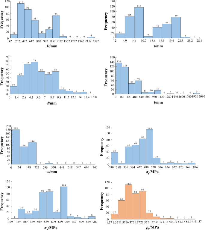
The statistical results of features.

Full size image