Accelerating the design and discovery of tribocorrosion-resistant metals by interfacing multiphysics modeling with machine learning and genetic algorithms
Introduction
Aluminum (Al) alloys are essential structural materials in a wide array of industries, including aerospace, civil infrastructure, and automotive sectors, due to their low density, high strength-to-weight ratio, good corrosion resistance, and excellent recyclability1,2,3. For example, with the demand for new energy and sustainability in the automotive field, Al alloys are gaining great interest as body parts in battery-powered electric vehicles4 due to their lightweight, high thermal conductivity5, and good corrosion resistance6. However, the inherent low mechanical strength of pure Al often poses challenges, especially in terms of wear resistance. To improve their wear resistance, Al can be hardened by alloying followed by appropriate heat treatment or aging to promote the formation of strengthening phases such as precipitates, constituent particles, and secondary phases7. Successful examples include the development of high-strength Al alloy series like 5xxx, 6xxx, and 7xxx, wherein precipitate-strengthening mechanisms play a pivotal role. Nonetheless, it is crucial to acknowledge a trade-off between mechanical and electrochemical properties often stems from such an alloying strategy. In essence, while these precipitates significantly enhance strength, they can inadvertently compromise corrosion resistance due to micro-galvanic coupling with the Al matrix, hastening the dissolution of the more anodic phase, typically the Al matrix itself8. Consequently, the endeavor to design Al alloys that concurrently exhibit high strength, wear resistance, and corrosion resistance presents a nontrivial materials design challenge.
In demanding operational environments, the degradation of Al alloys is often expedited by concurrent mechanical and corrosion attacks on metal surfaces, a phenomenon known as tribocorrosion. Consequently, designing Al alloys with robust tribocorrosion resistance is imperative to ensure the reliability and durability of Al alloy products in real-world applications. This intricate failure mechanism stems from the interplay of wear, corrosion, and wear-corrosion synergy9,10,11,12. Various material properties, loading conditions, and environmental factors—such as temperature, pressure, and corrosive agents—exert influence on tribocorrosion rates by affecting plastic deformation and corrosion product characteristics13. Generally, tribocorrosion exacerbates material deterioration and eventual failure through synergistic effects, profoundly compromising structural integrity and service longevity14. The stresses at the contacting asperities not only plastically deform the surface material, leading to the formation of wear debris, but also enhance localized corrosion on the wear track11,15,16. Notably, certain passive metals like stainless steel exhibit a counterintuitive negative stress-corrosion synergy, where corrosion-induced passive layers mitigate wear during tribocorrosion, thus reducing material loss17. However, in the case of Al alloys, such wear-corrosion synergy has often been found to enhance the corrosion process and accelerate total material loss18,19,20,21,22. In other words, the total material loss during tribocorrosion was found to be higher than the sum of pure wear and corrosion11,15,16. For example, Vieira et al.21 studied the tribocorrosion resistance of Al alloys in NaCl and NaNO3 solutions and proposed a theory attributing the enhanced localized corrosion to the galvanic coupling between the passive area and depassivated wear track during tribocorrosion. The worn area became depassivated while the unworn surface remained passivated. In our previous experimental study on Al-Mn alloys23, we found that the alloying concentration also affected the wear-corrosion synergy. The volume loss due to wear-corrosion synergy is higher in Al-20 at.%Mn than that of Al-5 at.%Mn even though the former exhibits better mechanical properties and corrosion resistance24,25. The physical origin of wear-corrosion synergy comes from two terms in Al alloys: (1) wear-accelerated corrosion and (2) corrosion-accelerated wear. The origin of wear-accelerated corrosion is confirmed by an increase in the current flow through the metal/electrolyte interface recorded on Al surfaces during tribocorrosion23. The current remains at an elevated level in order to sustain the imposed passive potential until the end of the test when the current restored to its original value due to subsequent repassivation of the worn area. For corrosion-accelerated wear, the passive oxide film, predominantly composed of alumina (Al2O3), paradoxically possesses high abrasiveness due to its low ionic potential26. During tribocorrosion of Al alloys, the wear debris containing abrasive corrosion products exacerbates material loss, fostering a positive stress-corrosion synergy, as observed in Al-Mn systems27,28,29. In other words, this previous study showed that materials with good mechanical and corrosion properties could still experience high material loss due to wear-corrosion synergy. Towards the design of high tribocorrosion resistance, it is thus essential to understand how various mechanical (e.g., Young’s modulus, yield strength, hardness) and electrochemical (e.g., exchange current density, Tafel slopes of the anodic and cathodic reactions) properties simultaneously affect the material loss from wear, corrosion, and the wear-corrosion synergy.
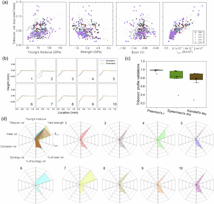
To date, tribocorrosion and wear-corrosion synergy are still poorly understood due to the very limited experimental data reported so far. We performed a literature survey of all tribocorrosion and erosion-corrosion studies from the papers published to date and found only a small fraction of tribocorrosion papers reported both mechanical and electrochemical properties. Almost 50 years of research worldwide has resulted in only about 300 such data points, upon which the property-performance, for example, the hardness-tribocorrosion rate relationship can be established. Figure 1 summarizes the hardness vs. tribocorrosion rate (i.e., the total volume loss divided by the sliding distance and the applied load) of stainless steel, aluminum alloys, CoCrMo, diamond-like carbon (DLC) on steel, and titanium alloys during tribocorrosion in 0.1–1.0 M NaCl solution from literature survey to date (1960–2024) using Scopus database. Interestingly, the data shows that the tribocorrosion rate does not show an inverse relationship with the hardness, which is predicted by the well-known Archard’s law in pure wear condition30. The scatter of the data further signifies the importance of understanding the synergy between multiple material properties on the overall tribocorrosion behavior.
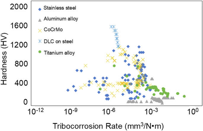
Summary of experimentally measured hardness vs. tribocorrosion rate of stainless steel, aluminum alloys, CoCrMo, diamond-like carbon (DLC) on steel, and titanium alloys during tribocorrosion in 0.1–1.0 M NaCl solution from literature survey to date (1960–2024) using Scopus database. The tribocorrosion rate is calculated using the total volume loss (mm3) normalized by the sliding distance (m) and applied load (N) for easy comparison among papers using different testing conditions.
To overcome the cost and time constraints in experimental studies, finite element analysis (FEA) modeling turns out to be a great alternative tool to study the complex and multifaceted phenomenon of tribocorrosion31,32,33,34,35. Our previous work has developed a multiphysics FEA model to simulate the stress and strain distribution, as well as the chemical and electrochemical reactions that occur in Al-Mn alloys during tribocorrosion, which is validated by experimental results32,36. Recently, we also demonstrated that such models can accurately predict the tribocorrosion current evolution of single crystal Al with different crystallographic orientations by considering the local lattice reorientation, galvanic coupling between the worn and unworn areas, as well as effects of subsurface dislocation on surface corrosion kinetics37. None of these fundamental insights could be gained through experiments alone. Using such experimentally validated FEA models, it is possible to predict the tribocorrosion performance of Al metals with high fidelity and quantify the material loss from pure wear, pure corrosion, and wear-corrosion synergy as a function of multiple material properties, such as alloy composition32, microstructure37, and surface finish38,39.
In this work, we use the experimentally validated high-fidelity FEA model36 to calculate the tribocorrosion rate as a function of six key material properties. Such data is then used for machine learning (ML) to accelerate the material design for outstanding tribocorrosion resistance. Recently, ML algorithms become increasingly popular in materials research to solve complex problems and make data-driven decisions40,41,42,43,44. These algorithms can learn complex patterns and relationships from datasets, allowing researchers to make more accurate predictions about the behavior of materials under complex conditions45,46,47,48,49. ML approaches offer several advantages, including increased efficiency, predictive power, adaptability, and the ability to uncover new insights and relationships in data that may not be apparent to physical-based models. As such, ML algorithms are poised to play an increasingly important role in tribocorrosion research and the design of tribocorrosion-resistant materials for harsh environments. By combining the ML algorithm with FEA models, a comprehensive understanding of the tribocorrosion phenomenon can be gained to optimize multiple material properties for tailored applications.
Several ML tools have been employed for a variety of tribology-related tasks, including but not limited to predicting wear rate50,51,52, designing functional materials53,54,55, estimating surface roughness56,57,58, and classifying wear particles59,60,61. Moreover, the integration of genetic algorithms (GA)62,63 with ML has been employed to enhance the pace of material discovery64,65,66. To the best of our knowledge, this work is the first attempt to use it in the tribocorrosion field, where the added physics of metal corrosion and wear-corrosion synergy renders it a highly challenging materials design and optimization problem. Herein, we present a novel approach to accelerate the design and discovery of tribocorrosion-resistant Al alloys by interfacing multiphysics FEA modeling with ML and GA. Specifically, this study establishes an ensemble artificial neural network (ANN) model that predicts tribocorroded surface profiles and total material loss of Al alloys with a wide spectrum of design parameters, encompassing mechanical and electrochemical properties previously unexplored experimentally. The uncertainty of predictions is quantified using the ensemble method, while a genetic algorithm is used to optimize the Al alloy properties by searching and identifying the optimal combination of mechanical and electrochemical properties. The data-driven model trained using a limited number (100 cases) of FEA simulations has enabled accurate predictions of material loss, with a mean absolute percentage error consistently below 10%. Moreover, the model deciphers the impacts of individual design parameters on material loss and achieves optimal material design within just three generations, effectively fulfilling the specific criterion of minimal material loss. This innovative approach shows immense promise in the domain of designing metals resistant to tribocorrosion, expanding its applicability beyond the focus on Al alloys examined in this study.
Results and discussion
Machine-learning-enabled workflow for designing tribocorrosion-resistant materials
The developed predictive modeling framework for optimizing material design for tribocorrosion resistance is structured into three main components: data preparation and preprocessing, training of the ANN model, and utilization of the ANN model in conjunction with GAs. Figure 2 illustrates the workflow visually. To prepare the training data, a Design of Experiment (DoE) was established within a defined parameter space (detailed in the next section). Subsequently, simulations of all cases were conducted using an FEA-based tribocorrosion model, resulting in a comprehensive training dataset for the ANN model. The ANN model consists of three modules: the strain module, the wear module, and the corrosion module. After training, the model undergoes an uncertainty test, and additional FEA simulations were performed in areas of high uncertainty to enhance the ANN model’s performance. Finally, a high-throughput method was used to generate a material loss map, and the optimal material design for a specific application was determined through the use of GAs.
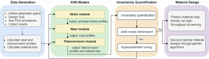
A Design of Experiment (DoE) prepares data and trains an ensemble ANN model with strain, wear, and corrosion modules, followed by an uncertainty test. High-throughput material loss mapping and GAs are employed for optimal material design.
FEA modeling of tribocorrosion in aluminum alloys
In this study, we adapted a developed FEA tribocorrosion model32 designed for Al-Mn alloys to simulate the behavior of a diverse range of Al alloys exhibiting comparable electrochemical characteristics but varying mechanical properties. The tribocorrosion behavior of Al-based alloys was measured and modeled using a ball-on-plate configuration in a 0.6 M NaCl solution, as shown schematically in Fig. 3a. In the experimental setup, an Al alloy plate is subjected to wear against a counter body consisting of a 4 mm diameter alumina ball23. The electrochemical response was measured using a 3-electrode setup, with the Al alloy serving as the working electrode (WE), along with mixed metal oxide coated titanium mesh and a commercial silver-silver chloride electrode (1 M KCl internal solution) serving as the counter (CE) and reference electrodes (RE), respectively. Throughout the tribocorrosion experiment, the Al plate undergoes concurrent wear and corrosion. Subsequently, material loss due to tribocorrosion is quantified through surface profilometry analysis of the wear track. The experimentally measured tribocorrosion rates were then used to validate the FEA model. The setup and experimental validation of the the FEA tribocorrosion model are comprehensively outlined in the “Methods” section and detailed in Supplemental Materials section 2.
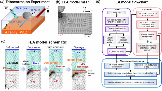
a A 3D schematic of the experimental tribocorrosion setup using a ball-on-plate configuration in 0.6 M NaCl aqueous solution, where WE (Al alloy), RE, and CE represent the working, reference, and counter electrode respectively. b FEA model geometry and mesh. c FEA model schematic and d flowchart where the worn surfaces are used as the input surface profile for the subsequent tribocorrosion simulation.
Figure 3b shows the FEA model geometry and mesh, which was constructed based on the experimental setup in Fig. 3a. The multiphysics nature of this model is that it combines wear and corrosion processes, plastic deformation, wear debris generation, and accounts for the electrochemical kinetics of the working electrode (i.e., Al alloy) from experimental measurements. Figure 3c, d provides a summary of the model schematic and flowchart, where the initial intact flat sample surface first experiences wear deformation, followed by pure corrosion on both worn and unworn surfaces, and finally, additional material loss due to wear-corrosion synergy. Prior to modeling the pure wear deformation, the mechanical response of this model was validated using experimentally measured nanoindentation results, and the contact mechanics were validated using Hertzian contact theory67 (see Supplemental Materials section 3). The wear-corrosion synergy in tribocorrosion was simulated by integrating the influence of mechanical deformation on electrochemical behavior. Specifically, the shift in anodic potential (φa) from its equilibrium value (φa0) is presumed to occur cathodically, depending on both elastic and plastic strain. Using this model, the FEA model predicted tribocorrosion volume loss of Al-Mn alloys, including both the mechanical (Vmech) and chemical wear (Vchem) during tribocorrosion, are in great agreement with those measured experimentally32. Additionally, the uncertainty quantification was carried out to evaluate the accuracy of the FEA model (see Supplemental Materials section 3). The model details, such as the governing equations and boundary conditions, can be found in the “Methods” section and the Supplemental Materials section 2.
This FEA model consists of six key material parameter inputs, including Young’s modulus (E), yield strength (σy), anodic Tafel slope (βa), cathodic Tafel slope (βc), anodic current density (ia), and cathodic current density (ic). A DoE approach is established to explore the huge parameter space, with each input parameter having five levels over its entire range to conduct the FEA simulations. The resulting 100 by 6 matrixes are plotted into a scatter plot as demonstrated in Fig. 4a while an additional 20 simulation cases within the training dataset parameter space serve as unseen validation cases. A t-SNE plot was generated to verify that all unseen cases are fully enclosed within the distribution of the training cases. The plot shows no overlap between the two groups and confirms that no unseen cases extend beyond the bounds of the training parameter space. This ensures that the unseen cases represent interpolations within the explored parameter space, rather than extrapolations beyond it. The t-SNE plot is provided in the Supplementary Materials as Fig. S8. Specifically, motivated by prior experimental results of Al alloys (see Supplemental Materials Section 1 for a summary of mechanical and corrosion properties of Al alloys from the literature survey), E and σy were varied from 55 to 95 GPa, and 1 to 5 GPa, respectively. βa and βc were varied from 0.25 to 0.29 and −0.29 to −0.25 V/decade, respectively. ia and ic were both varied from 1 × 10⁻¹⁰ to 5 × 10⁻¹⁰ A/cm2, respectively. In addition to these six parameters, corrosion potential (Ecorr) and corrosion current (icorr) were calculated based on the four electrochemical parameters (βa, βc, ia, and ic) and the equilibrium corrosion potential for Al (the anodic reaction) and hydrogen generation (the cathodic reaction), as shown in Fig. 4b. Ecorr and icorr provide a simpler and more practical way of characterizing the corrosion behavior, as they are more directly related to the overall corrosion rate.
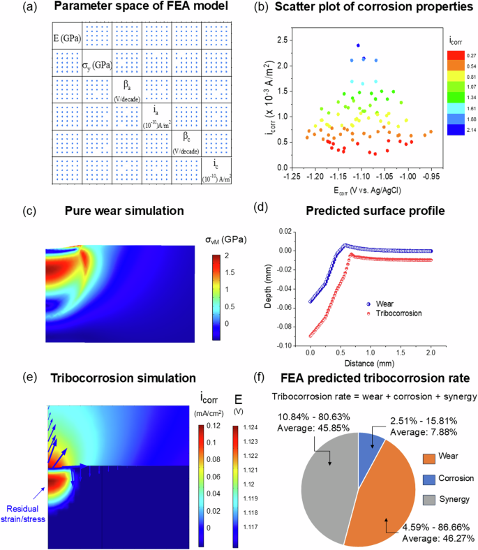
a The parameter space used in the tribocorrosion FEA model, where E (GPa) is the elastic modulus, σy (GPa) is the yield strength, βa, βc are the anodic and cathodic Tafel slope respectively, and ia, and ic are the anodic and cathodic exchange current density respectively. Each parameter has 5 levels of values. b Scatter plots of the corrosion current (icorr) and potential (Ecorr) calculated from the four electrochemical parameters (βa, βc, ia, and ic) and equilibrium potentials of the anodic and cathodic reactions. Typical FEA results of the c worn, d surface profiles, e tribocorroded surface, and f total tribocorrosion rate (material volume loss) from pure wear, corrosion, and wear-corrosion synergy of Al alloy (all FEA results from raw data are provided in Supplemental data.xls.).
Figure 4c–f summarizes the key FEA results. It has been found that subsurface residual strain develops within the wear track even after the indenter has left (Fig. 4c). Such areas are depassivated, thus showing a higher corrosion rate than those unworn regions (see the magnitude of arrows in Fig. 4e, which is proportional to local current density), which results in more material loss within the wear track area (e.g., distance of 0–0.5 mm in Fig. 4d) than that of the unworn region (distance 0.5–2.0 mm in Fig. 4d), indicating a positive synergy between wear and corrosion. Figure 4f shows the breakdown of total tribocorrosion rate (material volume loss) into contributions from pure wear, corrosion, and wear-corrosion synergy, namely, T = W0 + C0 + S. All FEA results are provided in Supplemental data.xls file. The tribocorrosion rate is primarily influenced by pure wear and synergy loss, with pure wear volume loss ranging from 10.84% to 80.63% and synergy loss ranging from 4.59% to 86.66%. On average, pure wear, pure corrosion, and synergy volume loss account for 45.85%, 7.88%, and 46.27%, respectively.
Figure 5a shows that during dry wear, the total wear rate is the smallest, with a low Young’s modulus (E) and high yield strength. Archard’s law is not obeyed here, and the wear rate does not increase linearly with 1/H as shown in Fig. 5b, yet monotonically with E/H, highlighting the importance of including the elastic response during the deformation process. In terms of tribocorrosion, the results of all 100 FEA simulations are summarized using the Radar plot depicted in Fig. 5c. This plot showcases the tribocorrosion volume loss, as well as the individual contributions from corrosion, wear, and synergy loss, along with their corresponding fractions. These parameters are plotted against two mechanical properties (Young’s modulus, yield strength) and two electrochemical properties (icorr and Ecorr). From the FEA simulation data, as depicted in Fig. 5c, the proportion of synergy material loss is notably higher, particularly when compared to corrosion material loss. In most cases, synergy material loss ranges from 30% to 60%, aligning closely with wear loss, whereas corrosion material loss accounts for only around 10%. Radar plots of 10 FEA results with the smallest tribocorrosion volume loss (i.e., tribocorrosion rate) are shown in Fig. 5d. Cases with minimum material loss demonstrate a variety of patterns, but they consistently feature high strength. Four patterns of the other three parameters emerge: The first pattern (case #1 and #2) involves an intermediate level of Young’s modulus and low icorr, resulting in a high wear volume loss and low synergy volume loss. The second pattern (case #3, #4, and #5) includes low Young’s modulus, and higher Ecorr and icorr, leading to minimal wear material loss but high synergy material loss. The third pattern (case #6 and #7) showcases high Young’s modulus and low icorr, resulting in higher wear material loss. The fourth pattern (case #8 and #9) is characterized by relatively high icorr and low Ecorr, along with low Young’s modulus, leading to high synergy material loss and low wear loss. Notably, there exists a complex interplay among mechanical and electrochemical material parameters that compromise wear and synergy material loss in case #10. Thus, it is imperative to map these trends more effectively to comprehend the intricate relationships and optimize material designs for minimizing material loss.
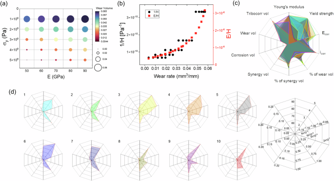
a Effects of mechanical properties on pure wear behavior of Al alloys. b Relationship of wear rate as a function of 1/H and E/H, where E and H represent elastic modulus and hardness respectively. c Radar plots of tribocorrosion, wear, corrosion, synergy volume loss, and their corresponding fractions as a function of 2 mechanical properties (Young’s modulus, yield strength) and 2 electrochemical properties (icorr and Ecorr). d Radar plots of 10 FEA results with the smallest tribocorrosion volume loss (i.e., tribocorrosion rate).
Ensemble ANN surrogate model for tribocorrosion behavior
The FEA simulation allows the calculation of material loss by analyzing the tribocorroded surface profile of the sample after tribocorrosion. The simulation input parameters and results are preprocessed into a training input file for the ML model, which includes surface profiles, material properties, electrochemical conditions, and spatial information. Figure 6a shows the ANN model for predicting tribocorrosion behavior consists of three sets of trained ANNs for uncertainty quantification using the ensemble method, with each set containing five ANNs. The preprocessed data from FEA simulations are fed to the first three ANNs, designed to predict the three principal strain profiles on the surface after wear, using input mechanical properties (i.e., Young’s modulus, and yield strength) and electrochemical properties (i.e., anodic and cathodic Tafel slopes, the anodic and cathodic exchange current density, icorr, and Ecorr) of the materials and testing conditions (i.e., indenter shape). Indenter shape is an important parameter in the ANN models, allowing for accurate prediction of the spatial distributions of principal strains, as it accounts for localized deformation effects. The fourth ANN predicts the cross-sectional wear profile based on the local strain information from the first three ANNs, linking the relationship between indenter shape, strain level, and wear profile. The final ANN predicts the cross-sectional tribocorrosion profile and calculates material loss using information from the first four ANNs. Notably, including indenter shape information in the ANN models can significantly improve the accuracy of the predicted local principal strains and overall predictions.
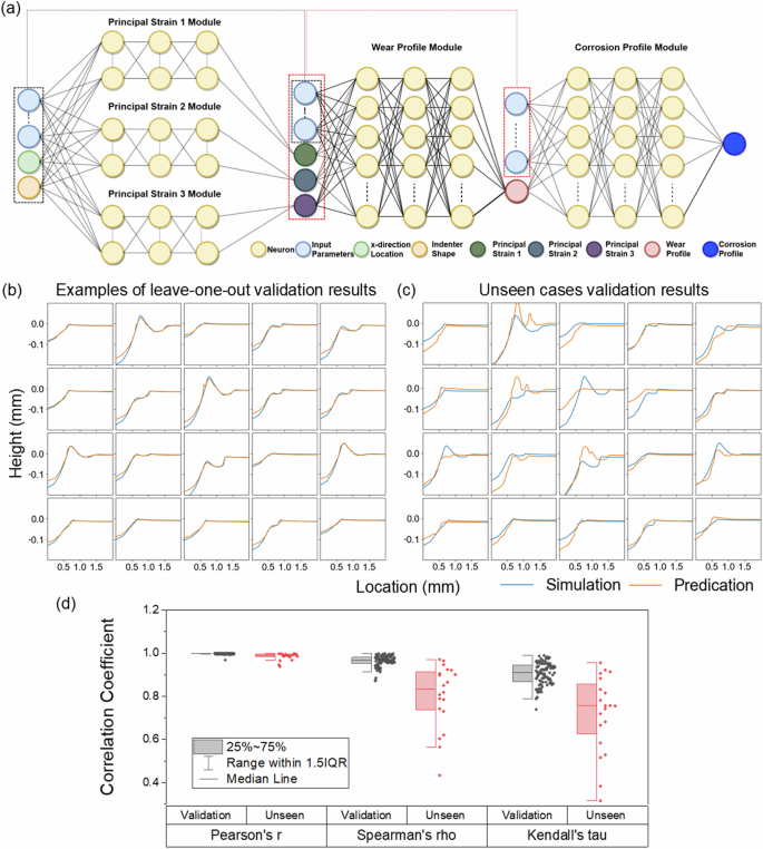
a The first three ANNs predict the principal strains after tribocorrosion based on various mechanical and electrochemical properties, and the fourth ANN predicts the cross-sectional wear profile. The final ANN predicts the tribocorroded surface profile and calculates the material loss. b, c The tribocorroded surface profiles of 20 cases of validation and unseen cases, respectively. d Quantitative analysis of the similarity between the simulation results and the ML predictions for validation and unseen cases. The analysis utilizes the Pearson correlation coefficient, spearman correlation coefficient, and Kendall’s tau.
Figure 6b displays the tribocorroded surface profiles of 20 training/validation cases. The simulated profile is obtained through the FEA model, whereas the predicted profile is generated through the ensemble ANN model using the validation (e.g., left-out) case. Profiles display a close resemblance to one another. The similarities between the two curves are evident in terms of their overall shape and amplitude. To perform a quantitative analysis of the similarity between the simulation results and the ANN predictions, we utilize the Pearson correlation coefficient68, spearman correlation coefficient68, and Kendall’s tau69, which are shown in Fig. 6d. The Pearson correlation coefficient, which measures the linear relationship between two variables, was found to be 0.99, indicating a very strong positive correlation between the simulated corrosion profile curves and the ML-predicted corrosion curves. The majority of the cases are very close to each other, with only one outlier at 0.94. The Spearman correlation coefficient, which is a non-parametric measure of correlation that is based on the ranks of the data, is found to be 0.94, indicating a strong positive correlation between the curves. There are 3 outliers between 0.85 and 0.9, suggesting that there may be some variability in the relationship between the curves for certain cases. Finally, Kendall’s tau, which is a non-parametric measure of correlation that is based on the concordance between the ranks of the data, is found to be 0.92, indicating a strong positive correlation between the curves. There is one outlier at 0.74, suggesting that there may be some disagreement between the curves for some cases. Overall, the high values of each of these coefficients suggest that the simulated corrosion profile curves and the ensemble ML model predicted corrosion curves are very similar. The high degree of similarity between the simulated and predicted profiles indicates the accuracy and reliability of the ensemble ANN model used to generate the predicted profile.
After validating the ensemble ANN model on 20 cases, it is evaluated on a set of 20 unseen cases to assess its generalizability. The results, presented in Fig. 6c, showed that although the model had limitations in predicting larger pile-ups or craters on the corrosion profiles, its overall accuracy remained satisfactory. Statistical analysis confirmed the high degree of similarity between the simulated and predicted corrosion profiles, with an average Pearson correlation coefficient of 0.99 and only two outliers of 0.93 and 0.92. The Spearman correlation coefficient of 0.83 and Kendall’s tau of 0.78 also indicated strong and moderate positive correlations, respectively, between the curves. Overall, the high values of these coefficients demonstrated the accuracy and reliability of the ensemble ML model, even for unseen cases.
ANN prediction of material loss and impact of material factors
The ensemble ANN model is further used for materials loss based on the tribocorroded surface profile. It has demonstrated satisfactory performance on both validation and unseen cases, indicating its ability to generalize and accurately predict new data. Examining the validation cases, the majority of the predicted material loss values from the ensemble ANN model closely resemble the simulated results, as shown in Fig. 7a. However, as the predicted material loss values increase, the difference between the ensemble model predictions and the simulated results also increases, with the ensemble model underestimating the material loss more significantly as the material loss becomes larger. Figure 7b shows that the ensemble model also performs well for most of the unseen cases, with the majority of the predicted material loss values being close to the corresponding simulated results, indicating satisfactory performance. However, larger differences between the predicted and simulated material loss values are observed for cases with higher levels of material loss, accompanied by an increase in uncertainty associated with the predictions. The difference in the material loss ranges between the validation cases (0–0.16) and the unseen cases (0–0.12) can likely be attributed to the fact that all unseen cases fall entirely within the parameter space defined by the training dataset. This suggests that the unseen cases represent interpolations within the parameter space rather than extrapolations into uncharted regions. As a result, the absence of edge cases in the unseen dataset naturally leads to a narrower range of material loss values. Figure 7c illustrates the mean absolute percentage error (MAPE) in the material loss for the validation cases has an average value of 0.1, with most cases having a MAPE value ranging between 0.06 and 0.13, suggesting that the ensemble ANN model is accurate in predicting the material loss for most cases. The MAPE values in the material loss for the unseen cases have an average value of 0.06, with the majority falling within the range of 0.015 to 0.17. While the model struggled to accurately predict the material loss for cases with significant topographical variations, the model’s performance has been considered satisfactory for identifying materials with less material loss ( < 0.1 mm2), which is the primary objective of this work.
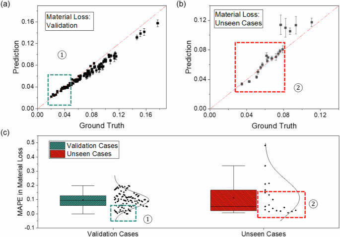
a, b The material loss predictions of leave-one-out validation and unseen cases, respectively. c Mean absolute percentage error (MAPE) of leave-one-out validation cases and unseen cases.
Utilizing the ensemble ANN model, we conducted a high-throughput study with 10,000 randomly generated input cases to delve into the expansive material parameter space and assess their impact on material loss. All four input parameters—Young’s modulus, strength, Ecorr, and icorr—are taken into account, with each range confined within the limits of the training dataset used for the ensemble ANN model. Figure 8a demonstrates that tribocorrosion volume loss slightly increases with Young’s modulus at each icorr level, suggesting that materials with higher modulus experience greater tribocorrosion. Conversely, Fig. 8b indicates that tribocorrosion volume loss decreases as strength increases, particularly when strength is less than 3 GPa, highlighting the importance of strength in resisting material loss. As illustrated in Fig. 8c, Ecorr alone does not show a clear trend at any icorr level with the tribocorrosion material loss, except at very high icorr levels, where increasing Ecorr leads to lower tribocorrosion material loss. This suggests that under extreme corrosion conditions, a more protective surface layer may form at higher Ecorr values, reducing material loss. Figure 8d shows a noticeable trend where higher icorr levels result in higher tribocorrosion volume loss at each E/H level, indicating the significant impact of corrosion current on material loss. The hardness values, denoted as H, are estimated here to be three times the yield strength70. Furthermore, we delve into the individual contributions to the total tribocorrosion volume loss, focusing on the interplay between the mechanical and electrochemical properties of the material in synergy material loss. Young’s modulus alone in Fig. 8e does not exhibit a clear trend at any icorr level with the synergy material loss, suggesting that Young’s modulus alone may not be a critical factor in determining synergy loss. Strength alone, as shown in Fig. 8f, increases with the synergy material loss at lower icorr levels, but the trend becomes less clear when icorr is high, implying that strength’s influence on synergy loss may be more pronounced under lower icorr conditions. The trends linked to mechanical properties are different from those of tribocorrosion material loss, as these properties influence tribocorrosion material loss through both wear and synergy contributions. On the electrochemical properties, Fig. 8g indicates that Ecorr alone does not have a clear trend at any icorr level with the synergy material loss, except at very high icorr levels, where an increasing Ecorr leads to lower synergy material loss. This trend aligns with tribocorrosion material loss, indicating that Ecorr may have a more pronounced impact on synergy loss under corrosion conditions, and influencing tribocorrosion material loss through synergy volume loss. Figure 8h demonstrates a monotonic increase in synergy volume loss with icorr. At low icorr levels, a higher E/H ratio correlates with reduced synergy volume loss, while at higher icorr levels, an intermediate E/H ratio yields the most significant synergy volume loss. This highlights a complex interplay between the E/H ratio and icorr. Wear volume loss, as depicted in Fig. 8i, directly affects tribocorrosion volume loss, with higher wear volume loss resulting in larger tribocorrosion volume loss at each icorr level, highlighting the importance of wear resistance in minimizing tribocorrosion. Conversely, corrosion volume loss, shown in Fig. 8j, is mostly affected by the icorr level, particularly affecting tribocorrosion volume loss more significantly when icorr is higher, indicating that controlling the corrosion rate is crucial in mitigating tribocorrosion. Finally, Fig. 8k illustrates the correlation between synergy loss and tribocorrosion loss at different levels of icorr. Interestingly, smaller synergy volume loss does not necessarily result in smaller tribocorrosion volume loss, especially when icorr levels are low. In fact, when icorr is low, a large synergy loss is more likely to lead to smaller tribocorrosion volume loss. This suggests a trade-off between synergy loss and wear loss within the parameter space.
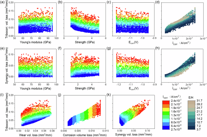
a–d Tribocorrosion materials loss plotted against Young’s modulus, strength, Ecorr, and icorr, respectively. e–h illustrate synergy material loss as a function of Young’s modulus, strength, Ecorr, and icorr, respectively. i–k display tribocorrosion loss relative to wear, corrosion, and synergy loss, respectively.
As indicated in the overview of experimentally measured tribocorrosion rates derived from our literature survey (Fig. 1) and other studies71,72, there is a generally inverse correlation between corrosion resistance and strength. Consequently, materials with higher strength typically exhibit reduced corrosion resistance, rendering them more susceptible to degradation and subsequent material loss. The lower strength allows corrosion processes to progress more rapidly, resulting in a more noticeable effect on material loss. On the other hand, icorr is the most influential factor studied, with increasing icorr leading to greater material loss. The rate of corrosion, as measured by icorr, is a crucial factor in determining the extent of material loss, higher icorr values indicate a greater rate of metal dissolution, leading to increased material loss. This is consistent with the well-established understanding that higher corrosion rates result in more significant degradation and material loss73,74. However, when delineating the individual contributions to tribocorrosion loss, it is found that a lower strength may contribute to a reduction in synergy loss, particularly when the corrosion current icorr is low. This trend aligns with our experimental findings, wherein the Al alloy with higher strength (Al-20 at .%Mn) exhibits greater synergy loss compared to the alloy with lower strength (Al-5 at .%Mn), despite having lower total and pure wear losses. This could be related to the wear-corrosion synergy described in Eq. (5), where a lower yield strength may result in a reduced cathodic shift from elastic deformation. Therefore, to minimize synergy material loss, it’s important to consider the interplay between material properties such as strength and corrosion resistance. Alloys with lower strength may be advantageous, particularly under low corrosion currents, as they can mitigate synergy loss. Furthermore, managing environmental conditions to lower corrosion rates can aid in mitigating synergy loss. This study underscores the importance of considering multiple factors when investigating material loss, as their interaction can significantly affect the outcome. The high-throughput approach using the ensemble ANN model enabled a more comprehensive analysis of the effects of these factors on material loss, providing valuable insights for future research and development of corrosion-resistant materials.
Material loss optimization through generic algorithm
Genetic algorithm (GA)-based optimization is employed to find the optimal set of input parameters that can minimize material loss. The ensemble ANN model is employed to generate 100 random cases independently from a uniform distribution for each factor within its training dataset parameter space to form the first generation of the GA population. As shown in Fig. 9a, the GA model can identify optimal material parameters resulting in low material loss as early as the third generation, requiring only 300 predictions. By the fifth generation, over 20 parameter combinations are identified. Interestingly, by the ninth generation, the GA model identified parameter combinations resulting in even lower material loss than those found by the high-throughput method. These findings show that the GA-based optimization approach with the combined ML model is an efficient and effective method for material optimization under tribocorrosion conditions.
a Evolution of each generation in parameter space of Young’s modulus, strength, Ecorr, and icorr. The effectiveness of the GA predictions is validated through b tribocorrosion profiles, c quantitative analysis of similarity with respect to FEA simulations. d The radar plots of 9 validated GA optimized cases (clockwise), including material properties Young’s modulus, yield strength, Ecorr, and icorr; and the resultant material losses (counterclockwise) such as tribocorrosion volume loss, wear, corrosion, synergy loss, and the fractions of synergy loss and wear loss.
To verify the accuracy of the GA predictions in finding optimal designs with low material loss, the top two parameter combinations resulting in minimal material loss from the last five generations were simulated using the multiphysics FEA model. Remarkably, four out of the ten cases predicted by the GA had lower material loss than the best prediction found by the high-throughput method. Figure 9b shows a close match between the simulated tribocorrosion profile curves and the GA-predicted tribocorrosion profile curves, with only two GA-predicted cases differing from the simulation validation cases. The average Spearman correlation coefficient is 0.84 with one outlier at 0.39, the average Kendall’s tau is 0.77 with one outlier at 0.28, and the Spearman correlation coefficient is 0.98 with two outliers at 0.90 and 0.95, indicating the high accuracy of the GA predictions, as shown in Fig. 9c. Overall, only one GA-predicted case (case #2) differed significantly from the simulation validation cases in terms of material loss. These results demonstrate that the GA is a reliable and effective tool for optimizing designs that minimize material loss in tribocorrosion studies.
Notably, the 9 validated GA optimized cases exhibit consistent ranges in the design parameter space for 4 material parameters, as shown in Fig. 9d. Specifically, Young’s modulus values fall within the lower range of 55 to 64 GPa, while strength values lie within the higher range of 3.8 to 5 GPa. In this study, the elastic modulus is varied across a range from 55 to 95 GPa, encompassing the typical elastic modulus range of conventional Al alloys (approximately 64–75 GPa)75,76. Similarly, Ecorr values are consistently within the medium range of −0.95 to −1.22 V, and icorr values remain in the lower range of 2.75 × 10⁻⁸ to 4 × 10⁻⁸ mA/mm2. While the high-throughput method reveals the general trend of the effects from each parameter, it is interesting that the “best” cases identified through GA optimization do not necessarily stem from the most extreme values within each parameter’s space (e.g., the highest strength values, lowest modulus, and the lowest icorr). It is clear that certain parameters can either enhance or reduce the impact of another parameter to some extent. For example, in cases #1, #6, and #8, relatively lower strength and higher modulus result in increased wear loss but reduced synergy loss, leading to an overall low tribocorrosion loss. Conversely, in case #7, when icorr is relatively high, the synergy loss dominates, necessitating very high strength and low modulus to reduce wear loss and maintain an overall minimal total loss. In cases #9 and #10, as compared to case #7, lower strength and reduced Ecorr contribute to a balance between wear loss and synergy loss. These trends underscore the importance of balancing wear and synergy material losses to minimize tribocorrosion material loss, aligning with the trends identified in the high-throughput analysis. Noteworthy that half of the GA parameters result in even lower material loss compared to the best FEA results by 5 to 10% in Fig. 5d, with 8 out of 9 GA cases exhibiting less material loss than the second-best FEA case. This suggests that the parameter combinations found by GA fall within a parameter space situated between those of the FEA parameters. It reveals trends that may not be readily discernible even with the use of DoE. This observation highlights the value of using GA, as it enables a more delicate exploration of parameter combinations and facilitates the balancing of different factors to identify the optimal combination.
In terms of computational time, simulating one new case with the FEA model takes an average of 20 min on a local workstation with an Intel XEON E5-2687W and 64 GB RAM. On the other hand, the ensemble ANN model is much more efficient and can predict 10,000 cases within 5 h. When combined with the GA algorithm, the optimal cases for material loss can be identified within 8 min, significantly improving design efficiency.
Traditional alloy design towards enhanced tribocorrosion resistance relies on low throughput and expensive experimental study to identify the optimum material properties. Due to the slow experimental approach, over the past 50 years or so, very limited property space, including both mechanical and electrochemical properties, has been explored. The literature survey conducted in this study shows that mechanical property (such as hardness) is not the only factor affecting the overall tribocorrosion rate, where the corrosion and wear-corrosion synergy also shows an important effect. During tribocorrosion of Al alloys, besides material loss from pure wear and corrosion, wear-corrosion synergy further exbate the material loss. In this work, using the experimentally validated FEA model, we show that under the invested tribocorrosion conditions, the wear-corrosion synergy could count for up to 80% of total material loss. Furthermore, we have identified combinations of properties that effectively reduce wear-corrosion synergy, a factor often overlooked in the design of wear- and corrosion-resistant alloys.
In summary, we develop a highly generalizable data-driven design framework for optimizing Al-based material design under tribocorrosion conditions by interfacing multiphysics modeling with ML and GA. The ensemble ANN model, consisting of three sub-model sets in series, provided accurate predictions of principal strains, wear profile, and tribocorrosion profile; and significantly reduced the time and computational demands compared to using only multiphysics FEA models. Through a high-throughput approach, we have found that icorr and strength both play significant roles in a total material loss to balance synergy and wear loss, underscoring the importance of considering multiple factors as their interaction can significantly affect the outcome. The GA-based optimization approach has further improved the efficiency of material design optimization, identifying optimal material designs with less material loss within minutes. The optimized designs have been validated by FEA simulations, indicating high accuracy in the optimization process. Overall, the ensemble ML model and GA-based optimization approach provide a highly efficient and accurate way of optimizing material design under tribocorrosion conditions, with promising applications in future material design research.
Methods
Multiphysics tribocorrosion finite element model
The multiphysics modeling framework involves wear, corrosion, and tribocorrosion processes in sequence, integrating plastic deformation, wear debris generation, and electrochemical kinetics, as illustrated in the flowchart (Fig. 3d). Before tribocorrosion simulation, typical abrasive wear behavior was studied by combining simulations of plastic deformation and the wear debris generation process. Specifically, the Al alloy and indenter have been identified as elastic-perfectly plastic materials without strain hardening during plastic deformation. In addition, to mimic the wear debris development, a strain-based material removal criterion was used, in which interacting asperities undergo highly plastic deformation and detach from the bulk. Based on the previous work77,78, it is assumed that the plastic strain ɛp induces material removal when it exceeds a critical value ɛc, which is set to be 0.0577 in this study. Thus, starting with the element closest to the surface, the algorithm systematically assesses the condition of each element along the z-direction. If the value of ɛp exceeds ɛc, signifying plastic deformation surpassing a critical level, the element is identified as worn and subsequently removed. The worn track surface profile is derived once this method evaluates all surface locations.
Apart from the wear process, the corrosion is simulated in 0.6 M NaCl aqueous solution. The current density (i) and the electrolyte potential (ϕ) were described by:
where Ql (e.g., Ql = 0 in a solution when positive ions are equal to negative ions) is the charge density in the solution. The conductivity of the solution σl is 0.05 S/cm in 0.6 M NaCl aqueous solution. In terms of local current density (iloc) at the electrode-electrolyte interface, the Tafel equation is used:
where the overpotential η is defined as (eta ={phi }_{{ext}}-{phi }_{{elec}}-{E}_{{eq}}). The external potential ϕext connected to the metal is equal to 0 in this study. ϕelec is the electrolyte potential and Eeq is the corresponding equilibrium potential of the reaction that occurred at the electrolyte-electrode interface. In addition, the boundary conditions are described as follows to calculate the local current density distribution:
Faraday’s law is applied to calculate the dissolution speed per unit area normal to the metal surface (Vn), as expressed by:
where n is the number of electrons transferred per ion, F is the Faraday’s constant ( = 96,485 C/mol), ρ is the metal density, and M is the molar mass. The electrolyte-electrode contact is set as a free-deforming surface, whereas the other sample boundaries are restricted displacement without deformation. The elements on the freely deforming surface can contract in accordance with the dissolution speed calculated from Eq. (4). The annotation of all boundary conditions can be found in Supplemental Materials Section 2.
On the other hand, the thickness-dependent electrical resistance of the surface film was applied to study the depassivation-repassivation process. Before the scratch starts, the thickness of the initial passive film (i.e., Al2O3 oxide film) is assumed to be 4 nm thick based on prior experimental results79, and the conductivity (σ) of Al2O3 is 1 × 10⁻¹² S/m. During tribocorrosion, it is assumed that the scratch removes this passive film and completely depassivates the surface. Thus, this oxide film thickness is reduced to 0, i.e., it is absent on the surface. Afterwards, this oxide film regrows on the surface, causing repassivation. In this model, the passive layer is treated as an electrical-resistant film whose resistance increases as the film grows thicker. Assuming at a certain location on the surface, the height loss of Al is d, and the accumulated passive layer thickness is thus 1.29 d based on the molar volume ratio of the oxide and its consumed metal (i.e., MAl2O3/MAl). With the dissolution of Al, the model generates a resistant barrier with local conductivity per unit area of 1.29σd. For the Al surface outside wear track where the passive layer is intact, a constant film thickness of 4 nm is used.
Lastly, the wear-corrosion synergistic effect in tribocorrosion is modeled by incorporating the change in electrochemical performance caused by mechanical deformation. Specifically, the anodic potential (φa) is assumed to shift cathodically from its equilibrium value (φa0) depending on the elastic and plastic strain following39,80:
where the second and third term are the shift of equilibrium potential due to elastic and plastic deformation, respectively. In Eq. (5), the stress σ is taken as the stress within the elastic deformation, and for the area that is plastically deformed, it equals the yield strength, Vm is the molar volume of aluminum (({V}_{m}=9.99times {10}^{-6}{m}^{3}/{mol})), T is the temperature (T = 298 K at room temperature), R is the ideal gas constant (R = (8.3145{rm{J}}/({rm{mol}}cdot {rm{K}})left)right.), εp is the effective plastic strain, and ({K}_{alpha }({varepsilon }_{p})) is a function denoting the dislocation density increment under plastic strain (εp), obtained by interpolating data from81. In the simulation for the tribocorrosion test, the deformed surface geometry and plastic strain after unloading obtained from wear simulation were imported as input to calculate φa following the Eq. (5) above at each single location on the sample surface. All the other parameters and settings are the same as the pure corrosion model. COMSOL Multiphysics software (version 5.3) has been used to set up the FEA model. The readers can refer to Wang et al.32 and Supplemental Materials Section 2 for the procedure of the FEA model.
Artificial neural network (ANN) model
The ANN model is written in Python, using a high-level API, Keras, which is provided by the TensorFlow platform82. Each ANN is trained using the leave-one-out method, as the validation method was driven by the small size of the dataset, which necessitated the maximization of available data for training. This method involves training the network on all but one of the 100 groups of input data and corresponding profiles and then using the trained network to predict the profile for the left-out group. This process is repeated for each group, resulting in 100 trained ANNs. The performance of each ANN is evaluated by comparing the predicted and actual profiles for the left-out group. While both the computational cost and potential risks of overfitting are higher, compared to alternative validation methods such as 5-fold and 10-fold cross-validation, the leave-one-out method allows for a lower error. In this study, the training RMSE for the leave-one-out method (approximately 0.035) was lower than that of 5-fold and 10-fold cross-validation (around 0.102), and additional measures were implemented to address the potential for overfitting. A comparison between the RMSE of 3 different cross-validation methods from strain module training can be found in the Supplementary Materials. These included the incorporation of dropout layers with rates between 0.1 and 0.3, which not only reduced overfitting but also improved the model’s robustness. The use of dropout layers lowered the training RMSE slightly (from 0.024 to 0.035) but significantly enhanced generalization, as reflected by the reduction in the mean absolute percentage error (MAPE) on unseen validation cases from 0.13 to 0.06. This improvement highlights the model’s ability to generalize effectively within the in-parameter space, ensuring reliable and accurate predictions of material loss. The structure of each module is comprised of 3 hidden layers with 10 to 200 nodes, respectively. The activation function used in all hidden layers is the rectified linear unit (ReLU). The learning rate of the model is set between 0.00125 to 0.01, and the hyperparameters are fine-tuned using the KerasTuner library to minimize the RMSE. This fine-tuning process optimizes the model’s performance and enhances its accuracy in predicting tribocorrosion material loss. More information on this process can be found in the Supplementary Materials.
Since each sub-model set has 5 ANNs that are trained individually, minimizing the error in the final result, the end-to-end training approach is used83. The separately trained ANNs are combined and trained as a single unit and allow the model to learn how to adjust each ANN’s output based on the next ANN’s predictions, resulting in more accurate final results. To implement this end-to-end training, a single model for each sub-model set that includes all five ANNs as layers is created. ANNs are combined as designed, and the final output will be the prediction of the last ANN, the tribocorrosion module. A loss function that takes into account the error of each ANN’s prediction and the error of its next ANN’s output is added for fine-tuning. Backpropagation is used to update the weights of all ANNs simultaneously. This fine-tuning reduces the risk of error accumulation that can occur when using multiple ANNs in succession. Additionally, the end-to-end approach allows the model to take advantage of the relationship between all ANNs and learn how to optimize their predictions together, potentially leading to improved accuracy in the final result.
Genetic algorithms (GA) and uncertainty quantification
GA is employed in this model to discover the most optimal material design. The model uses TensorFlow and numpy to implement a GA to find the best input data combination among Young’s modulus, strength, Ecorr, and icorr, resulting in the minimum material loss. As shown in Fig. 10, at the beginning of the GA process, the ranges for each input dataset are defined within the simulation DoE, and the population size and the number of generations are set to 100 and 10–20, respectively. The initial population is generated with random input combinations of the four properties, and the performance of each is evaluated individually. The GA is then used to select the top 25% of individuals with less material loss and low uncertainty. More specifically, the GA will search for individuals with lower material loss and reasonable uncertainty using the following equation: score = l × ϭ, where l is material loss, and ϭ is the level of uncertainty of predictions. Individuals with the bottom 25% scores will be considered the top individuals and be mutated by 0 to 10% to create a new population for the next generation. This process is repeated for the generations until a specified number of generations is reached or the minimum material loss is no longer decreasing significantly.
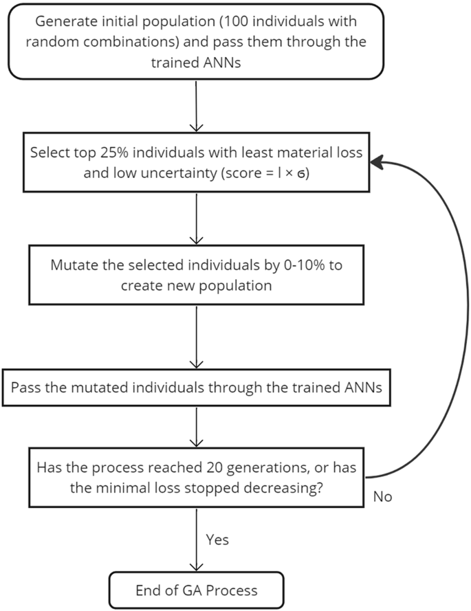
The GA process identifies optimal material properties by iteratively refining input parameters, combining material loss predictions with uncertainty quantification to achieve minimal tribocorrosion loss.
To ensure the reliability and usability of GA predictions, the model also uses an ensemble method that aims to estimate uncertainty in its predictions. The model comprises three sub-model sets, each of which is trained with the same training dataset but different hidden and dropout layers. Moreover, each of these sub-model sets predicts 2–5 times for each input dataset during the GA process. The predictions generated by these will be averaged, and the mean value will be used as the final prediction. Additionally, the standard deviation of these predictions is calculated to evaluate the uncertainty of the results. When GA selects the top individuals, the uncertainty of each individual is taken into account by assuming the final material loss equals the sum of the mean of predicted material loss and half of their standard deviation. By using this approach, a more robust prediction that takes into account the variability inherent in the data can be achieved.
Responses