Prediction of oxidation resistance of Ti-V-Cr burn resistant titanium alloy based on machine learning

The development and application of Ti-V-Cr burn-resistant titanium alloys is a direct and effective way to solve the “titanium fire” accident as well as the key basis for the successful design and production of advanced high thrust-to-weight ratio aeroengines^1,2,3,4. However, the lack of high-temperature oxidation resistance is one of the main reasons restricting its development. Alloying is one of the significant ways to improve the high-temperature oxidation resistance⁵. With the increase in the maximum operating temperature of the titanium alloys, the alloy composition system tends to be much more complicated⁶. In addition, it is necessary to accurately control the alloying elements based on the high-temperature oxidation resistance and mechanical properties of the alloys. Generally, the oxidation resistance properties of titanium alloys can be quantified and evaluated by correlating them with parabolic oxidation rate constant Kp according to Wagner’s theory of metal oxidation⁷.

The lower parabolic oxidation rate constant denotes the better oxidation resistance of alloys. Plenty of research, including isothermal oxidation weight gain experiments with different exposure durations, have been carried out to explore the effects of different alloying elements on the oxidation resistance of titanium alloys^6,8,9,10. STRINGER J. et al. originally studied the oxidation behavior of commercially pure titanium in the temperature range of 1073–1473 K in 1960¹¹. Kitashima T. et al. revealed the enhancement effect of Nb, Si, Zr, and Hf on the oxidation resistance of titanium alloy and the negative effect of Sn on its oxidation resistance by studying the oxidation behavior of binary α titanium alloy Ti-X (X = Al, Zr, Si, Hf, Nb, Ge, and Sn)^12,13. VOJTECH D. et al.¹⁴ and KNALSLOVA A. et al.¹⁵ demonstrated the effect of Si elements on the oxidation resistance of titanium alloys through oxidation experiments. Dai et al. summarized the high-temperature oxidation behavior experiments of titanium alloy and the effects of various alloying elements and coatings on the oxidation resistance of titanium alloy and titanium-aluminum alloy⁶. However, the oxidation weight gain experiment is time-consuming and laborious, and the oxidation resistance of the alloy can only be obtained at a specific combination of elements and oxidation temperature. Yang et al.¹² conducted an isothermal oxidation experiment for 500 h on nearly α titanium alloys containing Ga at 650, 700, and 750 °C. It was found that the oxidation kinetics of the alloys followed the parabolic oxidation rule at 650 °C and the cubic oxidation rule at 700 and 750 °C, respectively. Cruchley et al.¹⁶ obtained seven oxidation weight gain curves as long as 5000 h at different temperatures.

In order to tackle the issues of low efficiency and time-costing of traditional optimization methods based on experimental design, several theoretical calculation methods, namely density functional theory^17,18,19 including molecular dynamics simulation^20,21,22, phase field model^23,24,25, and phase diagram calculation (CALPHAD)^26,27,28 have been utilized to study the high-temperature oxidation behavior of titanium alloys. Ohler et al.²⁹ calculated the separation work at the interface between TiO₂ and titanium substrate by the DFT method, indicating that there is a strong bond between the substrate and the oxide film. Wu et al.³⁰ studied the diffusion of oxygen in α titanium and the impact of other solid solutions on oxygen diffusion. Bhattacharya et al.³¹ explored the effect of the Si element on the surface oxide film of titanium alloy through a molecular dynamics simulation method based on DFT. However, due to the limited computing ability and resources, such calculation methods have previously focused on studying the effects of individual elements on oxidation resistance and elucidating the oxidation mechanism of alloys^32,33,34,35. With the increase of alloying elements, the relationship between alloy properties and component elements tends to be much more complicated^36,37. Apart from that, there exists interactions between components which comes up with a greater challenge to the design and optimization of alloy components^38,39. The calculation and experimental verification costs of traditional alloy design methodologies are extremely high. Under this circumstance, new alloy composition design and performance prediction methods are still to be developed.

In recent years, the rapid development of machine learning and data science has provided new possibilities for the design of multi-component alloys⁴⁰. The concept of machine learning was first proposed by Samuel in 1959⁴¹. Based on a large number of known data and algorithms, machine learning mimics the human learning process and realizes the prediction of the relationship between alloy composition and macroscopic properties of materials through feature extraction and model training⁴². With the assistance of the trained machine learning model, a single objective or multi-objective optimization process is able to be carried out to obtain the most appropriate alloy composition combination⁴³. The active learning method inspired by machine learning and data statistics has a simple concept and clear logic, which can effectively reduce the calculation and time cost of alloy composition design⁴⁴. With respect to the machine learning algorithm for aeroengine titanium alloy, there are several specific characteristics. Firstly, Ti element can form a solid solution with Al, Nb, Cr, V, Zr, Sn, and other metal elements^33,45,46; Secondly, although the solid solubility of C, Si, N, O, and other nonmetallic elements is low, they can form precipitate phases in the substrate which has a significant effect on the plasticity and creep strength of the alloy^47,48,49,50. Thirdly, the phase transformation process of titanium alloy substrate is fairly complicated, while different alloying elements have distinct effects on the stability of phase structure⁵¹. Subsequently, alloying elements react with each other leading to the formation of complex multi-component compounds such as Ti₂AlNb and Ti₂AlC^52,53. Lastly, the number of alloying elements of high-temperature titanium alloys above 550 °C can reach 10 or even larger⁵⁴. These factors lead to a significantly complicated and implicit relationship between the element compositions and alloy properties of aeroengine titanium alloys. Therefore, the researchers modified the machine learning model by introducing special parameters and other methods to make it more suitable for titanium alloy systems. For example, Yang et al.⁵⁵ embedded the Mo equivalent and cluster equation into the model in the Ti-Mo-Nb-Zr-Sn-Ta alloy system, and five kinds of low-elastic β-Ti-alloys were designed by combining XGBoost with a genetic algorithm, which well predicted the influence of the change of Mo element content on the properties of titanium alloys. Among them, the Mo equivalent is closely related to the proportion of β phase in titanium alloy^56,57. The introduction of Mo equivalent can improve the perception of physical information in the model, and its expression is shown in equation (1).

In this work, the isothermal oxidation test experiments of Ti-V-Cr burn-resistant alloys were systematically carried out. Different machine learning models were established and trained based on experimental data and data accessed from the literature. The oxidation resistance mechanism of the Ti-V-Cr alloys was analyzed by combining the SHAP interpretability analysis, feature importance ranking, and material characterization results. Additionally, the Bayesian optimization algorithm was adopted to improve the performance of the models so that the models could accurately predict the oxidation resistance of different alloys. Through this study, the efficiency of the Ti-V-Cr alloy design process will be greatly improved. The Ti-V-Cr alloy properties database and accurate prediction models were established and verified by the comparison between the experimental results and predictions of machine learning models, which, to a great extent, provide significantly accurate guidance for Ti-V-Cr burn-resistant alloy composition design.

Performance of ML models

In the K-fold cross-validation, the average RMSE of the testing set was adopted as the return value of the objective function and the optimal hyperparameter combination in the model was searched in the direction of minimizing RMSE by BO. After obtaining the optimal solutions of hyperparameters of GBDT, BPNN, SVR, and XGBoost models, the machine learning model framework was built with them respectively. The K-fold cross-validation method was utilized to evaluate them again after training. Among them, the determination coefficients R² and RMSE introduced above were selected as the evaluation indexes of the model. The corresponding R², RMSE, and mean absolute error (MAE) of each model are shown in Table 1.

In addition, according to the results of the K-fold cross-validation method of the model, the scatter map of the predicted value and the actual value was drawn. Since the K-fold cross-validation method takes each fold as a testing set for prediction analysis, the result naturally traverses the entire dataset. Therefore, all the scatter points in the figure were used as testing sets, and lnk_p was predicted by the model, which is shown in Fig. 1. The bar chart below the scatter plot shows the difference between the predicted value and the actual value when all the samples are used as the test set, which is used to analyze the distribution of the true error of the model. Combined with the results of Table 1 and Fig. 1, the performance of four different models can be analyzed.

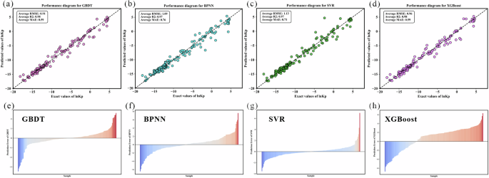
a Performance of GBDT, b BPNN, c SVR, d XGBoost, e error distribution of GBDT, f BPNN, g SVR, h XGBoost.

Full size image

GBDT model demonstrated excellent performance with an R² of 0.98, indicating a very high degree of fitting to the data. Lower RMSE (0.91) and MAE (0.59) compared to the other three models further illustrated the advantages of GBDT in forecasting accuracy and stability. This result is attributed to the continuously optimizing residuals of the GBDT model in the process of gradually building multiple decision trees thus improving the predictive power of the overall model. GBDT’s step-up mechanism can effectively handle nonlinear relationships and complex data structures.

The R² value of BPNN is 0.97, which is slightly lower than the GBDT model but still shows high fitting ability. However, its RMSE (1.09) and MAE (0.76) are relatively high, indicating that BPNN is inferior to GBDT in terms of prediction accuracy and error. BPNN can deal with complex nonlinear problems by optimizing weights through a backpropagation algorithm. Nevertheless, BPNN has high requirements on data volume and training time and it is easy to fall into local optimization resulting that its performance may not be as stable as GBDT in some cases.

The R² value of XGBoost is 0.98, which is comparable to GBDT, implying that it also has very high fitting capability. Its RMSE (0.96) and MAE (0.59) also show excellent performance in forecasting accuracy and stability. XGBoost is optimized on the basis of traditional GBDT using regularization processing to prevent overfitting and improve training speed through parallel computation. Its efficient tree structure construction and pruning mechanism make it especially good for processing large-scale data.

It can be concluded that GBDT and XGBoost have the best performance in all evaluation indicators demonstrating that they have obvious advantages in processing complex data structures and improving prediction accuracy. These two models are more appropriate for the dataset adopted in this study. In the following work, the GBDT model will be further sorted for feature importance and analyzed for the interpretability of the model.

Feature importance analysis

Feature importance analysis is a technique used to assess the extent to which input features influence the prediction results of a machine learning model. Calculating the contribution of individual features to the model output can help identify which features play a significant role in the model.

Firstly, the most influential features can be identified, thereby optimizing the feature set, removing redundant or irrelevant features, and improving the efficiency and accuracy of the model. Secondly, through feature importance analysis, the potential mechanism and hidden patterns in the data can be obtained to understand the problem domain further. In addition, feature importance analysis can improve the interpretability of the model making the model more transparent and reliable when applied to practical issues. Therefore, feature importance analysis is not only an important part of machine learning modeling, but also a powerful tool for making data-driven decisions.

Figure 2 shows the feature importance ranking diagram of GBDT and XGBoost models where the x-axis is the feature importance degree, and the y-axis denotes the feature name. In GBDT, the three most important characteristics are temperature, Ti content, and V content. In XGBoost model, besides temperature, Zr content and Cr content are the two most influential features. According to the Arrhenius equation, oxidation temperature should be the most significant feature in the oxidation process, which is consistent with the model analysis results. The V element forms a protective layer of V₂O₅ on the surface as it oxidizes, preventing further oxidation. The dense ZrO₂ oxide layer formed during the oxidation of Zr element can also protect the metal substrate from further oxidation. TiO₂ and Cr₂O₃ oxides formed by Ti and Cr elements are thermal stable at high temperatures which can reduce the oxidation rate and protect the substrate metal. Subsequently, the model analysis results can be compared with the experimental results to analyze the reliability of the model and provide guidance for the design of alloy composition.

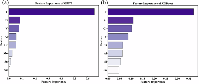
a GBDT, b XGBoost.

Full size image

Interpretability analysis of the model

SHapley Additive exPlanations (SHAP) is a game theory-based method for explaining the predictions of machine learning models. It provides a unified measure of the interpretability of the model by calculating the contribution value of each feature to the predicted result. SHAP values reflect the influence of each feature on the model output in different input cases helping to understand the decision mechanism of the model.

The necessity of SHAP interpretability analysis lies in:

1. (1)

   By quantifying the importance of features, SHAP can reveal the decision-making process of the model, making it more transparent and understandable.

2. (2)

   Help identify features that have a significant impact on prediction results and guide feature engineering and model optimization.

3. (3)

   Identifying potential model biases or complex relationships between features helps to find problems in the model and directions for improvement.

SHAP analysis plays a significant role in improving the interpretability, reliability, and validity of machine learning models and is a critical tool in data science and machine learning.

Figure 3 demonstrates the interpretability analysis of the XGBoost model using the SHAP method where the x-axis is the SHAP value, that is, the influence and contribution of each feature to the model output lnkp. The Y-axis is the name of each feature, sorted from top to bottom in order of the degree of contribution. The analysis results show that the higher the temperature, imply the greater the positive influence on the output lnkp. When the content of Ti and Al elements is higher, most SHAP is negative, indicating that the degree of negative influence on lnkp is greater and the oxidation resistance of the corresponding alloy is better. The higher the content of element V, the larger the lnkp output of the model is and the worse the oxidation resistance of the corresponding alloy is, which is similar to the experimental results. The SHAP value has both positive and negative of the higher the content of Cr element which is different from the rule obtained by the experiment and the specific reason needs to be further analyzed.

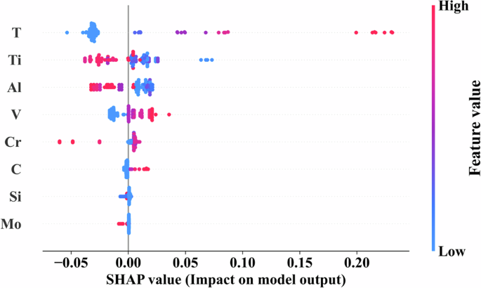
Force plot of the SHAP analysis for the XGBoost model.

Full size image

Results of oxidation experiments

The oxidation weight gain curve is a dynamic description of the alloy oxidation process. Based on the oxidation weight gain curve, the oxidation rate index and oxidation constant which measure the oxidation resistance of the target alloys can be calculated. This summary plots the oxidation weight gain curves for alloys and compares the oxidation resistance of alloys by comparing the shapes and relative positions of the curves. There were more than 60 groups of oxidation data obtained from the experiments, including the variation of V, Cr, and Al content and the corresponding results were demonstrated by the weight gain curves.

The data from the oxidation experiment are divided into three groups, and the average of the difference between the measured mass and the mass before oxidation is obtained as the oxidation gain.

The oxidation gain is the difference between the mass after oxidation and the mass before oxidation. The oxidation gain divided by the sample’s surface area gives the oxidation gain per unit surface area, as shown in Equation (2):

where M is the oxidation gain at the corresponding time and A is the total surface area of the sample.

Figure 4 shows the oxidation weight gain experiment of 1000 h. It can be seen from the figure that the oxidation weight gain of the listed kinds of Ti-V-Cr alloys meet the parabolic rule and conforms to Wagner oxidation theory. Therefore, it is reasonable to apply the parabolic oxidation rate constant as the model prediction index in the subsequent model.

The oxidative weight gain curve of the sample was plotted with time (h) as the horizontal coordinate and oxidative weight gain per unit surface area (g/m2) as the vertical coordinate. Tables 2–4 are the corresponding series and components of the alloys whose effects of Cr, V, and Al content on the oxidation resistance of the alloys were studied by using the control variable methodology and three sets of parallel experiments were carried out for each component with error calculated.

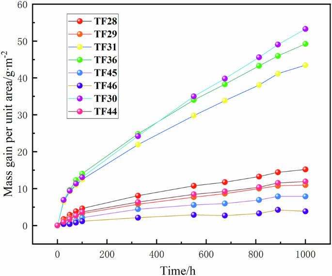
The oxidation weight gain curve of each component alloy at 1000 h.

Full size image

Non-consumable vacuum arc melting was carried out on the alloys in the table, and the samples were processed as standard samples for oxidation experiments. After the 100 h oxidation weight gain experiment, the oxidation weight gain curves of each alloy were shown in Fig. 5.

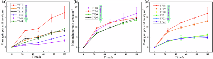
a Varying content of Cr, b Varying content of V, c Varying content of Al.

Full size image

Comparative analysis shows that other conditions remain unchanged, the higher the content of Cr in the experimental range, the better the high-temperature oxidation resistance of titanium alloy. When the mass fraction of V element is less than 0.3, the higher the content of V element, the better the high-temperature oxidation resistance of titanium alloy. When the mass fraction of V element reaches 0.3, the higher content of V element cannot improve the high-temperature oxidation resistance of titanium alloy. Only from the oxidation weight gain curve, the higher the Al content on the whole, the better the oxidation resistance of titanium alloy. However, when the content of Al element is higher than 3%, increasing the content of Al element can hardly increase the oxidation resistance of titanium alloy. It was noted that there was a data anomaly in the group of experiments with TF23, namely 6% Al content. The weight gain per unit area calculated by high-temperature oxidation for 100 h is smaller than that for 75 h. In theory, when the oxide film does not fall off, the oxidation weight gain will only become larger, not smaller. Therefore, this study speculated that there may be errors in the experiment process leading to oxidative shedding. To this end, the data of three sets of parallel experiments (oxidation gain per unit area: g/m²) were checked, as shown in Table 5.

It can be seen from Table 5 that the oxidation weight gain of the three groups of parallel experiments decreases during the oxidation period from 75 to 100 h, thus the error of experimental operation can be eliminated. The reasons for this phenomenon remain to be explained in the follow-up work.

Characterization analysis and mechanism discussion

The oxidized samples were analyzed by metallography, SEM and EDS. The oxidation film thickness of each alloy was calculated by scanning electron microscopy, and the oxidation rate constant calculated by the oxidation weight gain curve was used to evaluate the oxidation resistance of different alloy components. The oxidation resistance mechanism of Ti-V-Cr alloy was discussed based on the reports in the literature, and the influence of the change of the content of each alloy element on the oxidation resistance of the alloy was analyzed, and the reliability of GBDT and XGBoost models was verified by comparing with the analysis results obtained by the machine learning model.

Three alloys, TF12, TF18, and TF24, were selected for scanning electron microscopy, surface scan, and line scan energy spectrum analysis of their cross sections. The analysis results are as follows.

As can be seen from Fig. 6 of the section scanning electron microscope, the average thickness of the oxide film of the binary alloy TF12 (Ti-12.5Cr) containing only Cr element is 1.250 μm, which is thinner than that of the other alloys containing V and Al elements in the experiment, but the oxide film is not continuous, and the phenomenon of spalling and falling off of the oxide film is common. It has a certain effect on the oxidation resistance of the alloy. EDS results showed that the oxide film was composed of Ti and Cr oxides.

Combined with the analysis results of the machine learning model and the experimental law, the higher the content of Cr element, the better the corresponding oxidation resistance of the alloy, but too much Cr element (higher than 15%) will lead to the deterioration of the plasticity and thermal stability of the alloy. Considering the comprehensive mechanical properties, the recommended design range of the Cr element is about 15%, and the oxidation resistance of the alloy is better. At the same time, it also takes into account the requirements of mechanical properties.

Figure 6b shows the SEM and EDS characteristic results of Ti-20V-15Cr-1Al alloy. The average oxide film thickness is 5.329 μm. The oxide film is composed of Ti, V, Cr, and Al oxides, and the oxide content in the outer oxide layer of the oxide film is generally higher than that in the inner oxide layer near the matrix. The content of the Al element in the oxide film is similar to that in the matrix.

Figure 6c shows the SEM and EDS characterization results of Ti-25V-15Cr-1Al alloy. The average oxide film thickness is 6.446 μm. The oxide film is composed of oxides of Ti, V, Cr, and Al elements. The distribution of Al element in the oxide film has a polarization phenomenon. In the local high Al element region, the content of Ti is significantly lower than that in other regions of the oxide film, and the content of V and Cr elements is increased to a certain extent in this region, which may indicate the formation of a new multiphase. In order to understand the spatial distribution and concentration changes of each element in oxide film and matrix, the energy spectrum line scanning of these three alloys was further carried out.

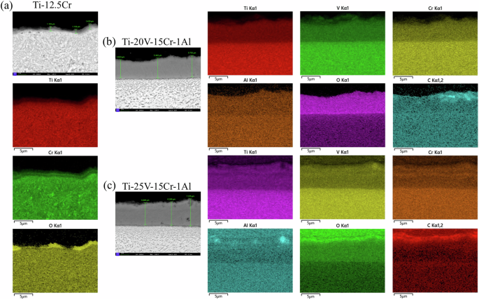
a TF12 (Ti-12.5Cr), b TF18(Ti-20V-15Cr-1A1), c TF24(Ti-25V-15Cr-1A1).

Full size image

Figure 7 shows the line sweep results of Ti-12.5Cr alloy. In the oxide film region, the content of oxygen elements gradually decreased from outside to inside, and was relatively low in the matrix, and the value of cps was close to 0. The content of Ti element increased gradually from outside to inside the oxide film. The content of Cr was different from its changing trend, from outside to inside, it increased first and then decreased, and remained stable in the matrix.

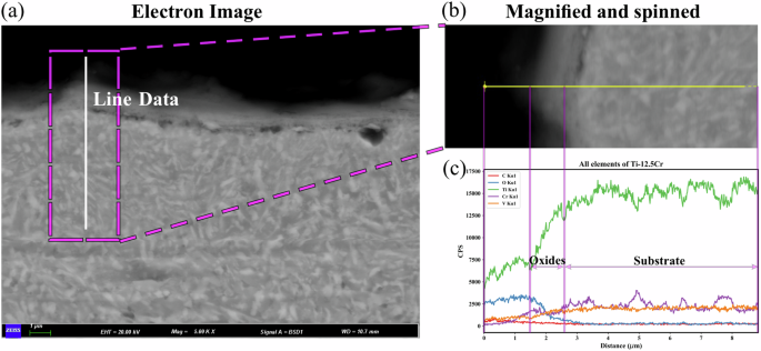
a Electron image, b magnification of rectangled area, c variation of content along the plotted line.

Full size image

Figure 8 shows the line scanning results of Ti-20V-15Cr-1Al alloy. In the oxide film region, the content of O element remains at a relatively stable level. The contents of the V element and Cr element were maintained at a stable level in the oxide film.

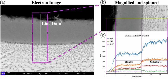
a Electron image, b magnification of rectangled area, c variation of content along the plotted line.

Full size image

Figure 9 shows the line scanning results of Ti-25V-15Cr-1Al alloy, which are similar to the results of Ti-20V-15Cr-1Al. In the oxide film region, the content of O element remained at a relatively stable level. The content of the V element and Cr element in the oxide film increased steadily, and the increasing rate was slow. Different from Ti-12.5Cr alloy, the content of Ti element in the oxide film is more evenly distributed, and there is no obvious upward trend, and only a sudden increase occurs near the matrix.

The following discussions and conclusions can be drawn from the prediction model and experimental study of the oxidation resistance of Ti-V-Cr flame retardant titanium alloy. (1) A prediction model for the oxidation resistance of Ti-V-Cr flame retardant titanium alloy was constructed. Due to sparse data when oxidation gain was used as the prediction index, the R² of the model reached only 0.81, and the corresponding algorithm was ANN; When the parabolic oxidation rate constant lnkp was used as the predictor, the data quality was higher, the R² determination coefficient of the model reached 0.98, and the maximum error was only 6.40%. The corresponding algorithm was the extreme gradient lifting decision tree XGBoost. (2) In the current oxidation experiment, the higher the content of Cr, the better the high-temperature oxidation resistance of titanium alloy. When the mass fraction of V element is less than 30%, the higher the content of V element, the better the oxidation resistance of the alloy. When the mass fraction of V element reaches 30%, the higher the content of V element can not significantly improve the high-temperature oxidation resistance of titanium alloy. The higher the content of Al, the better the oxidation resistance of the corresponding titanium alloy. (3) The feature importance and SHAP interpretability analysis results of the machine learning model show that the factors that significantly affect the parabolic oxidation rate constant of the alloy are temperature, Ti content, Al content, V content, and Cr content. SHAP analysis shows that Ti and Al elements are beneficial to improving the oxidation resistance of the alloy. The oxidation resistance of the alloy will be reduced with the increase of V content. The SHAP value of the Cr element is positive and negative, which shows that the anti-oxidation performance can be improved as a whole, which is consistent with the experimental law.

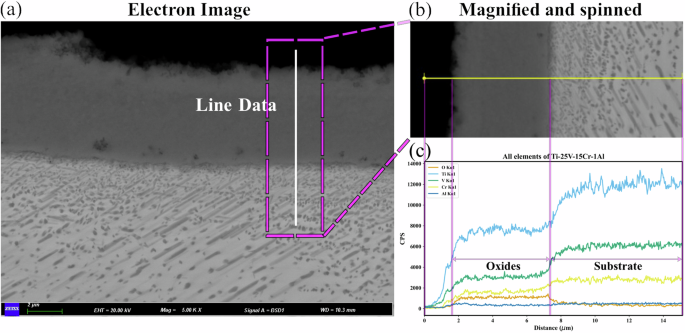
a Electron image, b magnification of rectangled area, c variation of content along the plotted line.

Full size image

Data source and quality

So as to tackle the issue of sparse data of isothermal oxidation experiments when only the Ti-V-Cr alloy system is considered. This work investigated and collected the isothermal oxidation data of high-temperature titanium alloys above 550 °C and high entropy alloys containing Ti at different temperatures that meet Wagner’s metal oxidation theory and basically obey the parabolic oxidation rule in literature. Apart from that, more than 60 groups of isothermal oxidation experiments at 600 °C were carried out, varying the content of V, Cr, and Al in the Ti-V-Cr alloy system according to the oxidation weight gain method. The results were included in the database combined with the data accessed from literature. The final database contains 156 sets of data^{6,58,59,60,61,62,63,64,65,66,67,68,69,70,71}, each of which includes element composition (wt,%), oxidation temperature (°C), oxidation time (h), oxidation weight gain per unit area (mg/cm²), and parabolic oxidation rate constant k_p. The parabolic oxidation rate constant k_p is an intuitional and quantitative index to assess the oxidation resistance of specific alloys, whereas the oxidation weight gain per unit area can only linearly obtain the overall oxidation resistance during a time period. The oxidation time and oxidation weight gain per unit area were therefore utilized only to calculate the k_p values in this research. The machine learning models adopted 19 features (including 18 alloy composition and oxidation temperature) as inputs and parabolic oxidation rate constant k_p as the prediction target.

After the database was established, the units of the data were converted. The alloy atomic ratio content (at,%) was uniformly converted into a mass fraction (wt%); The unit of oxidation temperature is uniformly converted to °C. The unit of the parabolic oxidation rate constant k_p is unified to mg²cm⁻⁴s⁻¹.

All data needed to be normalized after being converted into unified units. The purpose of normalization processing is to scale the data with different characteristics into the same range. Through this approach, the model training could be more stable and efficient. The accuracy of the model is able to be improved to a certain extent. In this paper, the Min-Max normalization method was used to scale the data to the range of 0 and 1. The Min-Max normalization equation is shown in equation (3)

where ({x}^{{prime} }) represents the normalized value of the data; (x) is the original value; ({x}_{min }) is the minimum value of the feature; ({x}_{m{ax}}) indicates the maximum value of the feature.

Due to the magnitude of feature k_p being on the order of 10⁻⁶ to 10⁻⁷ and the significant difference between its minimum and maximum values, a natural logarithm transformation (lnk_p) was applied resulting in a range of −18.13 to 4.61 for lnk_p. Table 6 presents statistical information for all features in the dataset, including lnk_p as the target for machine learning models.

The distribution of the dataset significantly impacts the accuracy and robustness of models. In addition to the information revealed in Table 6. Table 7 demonstrates the data distribution information of the whole 19 features, which are the inputs of machine learning models as well.

So as to have an intuitional knowledge about the data distribution of both 19 features and the target lnk_p, a 3D scatter diagram of all the samples within the dataset after being processed by PCA, which includes the information of all 19 features as well (Fig. 10) was plotted. Figure 11 illustrates the distribution of lnk_p. Except for the range of −15 to −10 (data obtained in experiments of this study), the values of lnk_p are approximately uniformly distributed across the intervals facilitating the subsequent model establishment.

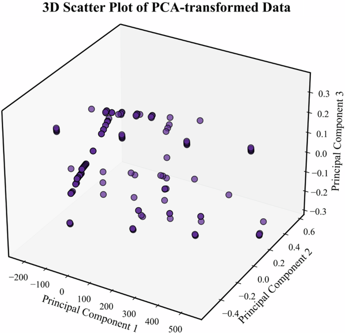
Three-dimensional demonstration of data distribution of all samples, including 19 features after PCA.

Full size image

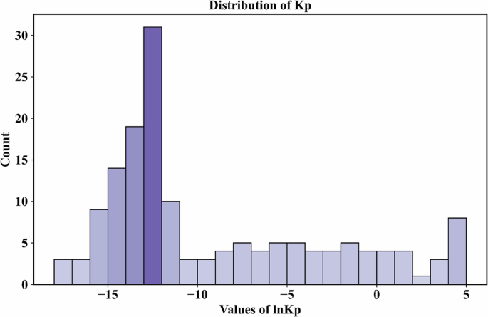
Distribution of lnkp (Values vs. Count s of lnkp in Dataset).

Full size image

Model establishment and training

In this research, machine learning models were developed using both single learners algorithm (BPNN, SVR) and ensemble learners algorithm (GBDT, XGBoost, RF). Their prediction performance was compared horizontally. The evaluation metrics for the machine learning models were the coefficient of determination R² and root mean squared error (RMSE). RMSE is a commonly utilized metric to assess the prediction performance of regression models representing the square root of the average squared difference between predicted and actual values. A lower RMSE indicates better model performance with the calculation formula shown in Equation (4):

where n represents the total number of samples which is the number of observations in the dataset as well; y_i denotes the actual value of the ith observation.

The coefficient of determination R², also known as the goodness of fitting, measures the proportion of variance in the dependent variable that is predicted from the independent variables. The R² value ranges from 0 to 1 with values closer to 1 indicating a better fit of the model to the data. It is calculated as shown in equation (5).

In the equations, (S{S}_{{res}}) represents the residual sum of squares, and (S{S}_{{tot}}) represents the total sum of squares. These are calculated using the following formulas, as shown in equations (6) and (7):

where (bar{y}) is the average value of the actual value.

All the machine learning models included in this study were verified by K-fold crossover validation method. The K-fold crossover validation method is often used to evaluate machine learning models with small data sets. In the data partitioning stage, the method divides the dataset into K subsets of roughly equal size called collapses. In the model training and verification stage, for each fold, each fold is taken as the verification set, respectively and the remaining K-1 folds are taken as the training set. After the training is complete, the remaining fold (validation set) is used to evaluate the performance of the model. This process is repeated K times while using a different fold as the verification set at each time to make sure that each fold is utilized as a validation set once. After all K tests, the performance of the model on each verification set is averaged to get the overall performance evaluation of the model. There are several advantages of the K-fold method:

1. (a)

   Throughout the process, the model was trained and validated, transversing all the data, and every data point was used for both training and validation, making the most of the limited data available;

2. (b)

   Through multiple training and verification, the performance of the model can be evaluated more reliably and the contingencies caused by data division can be avoided. Additionally, the generalization ability and accuracy of the model can be improved.

Bayesian optimization on hyperparameters of machine learning model

Bayesian optimization(BO) is an effective method for optimizing hyperparameters of machine learning models. It is especially suitable for high-dimensional and non-convex optimization problems. Through this method, the hyperparameter combinations close to global optimal solutions can be found in relatively few iterations. BO works by building a surrogate model (usually a Parzen estimator of a Gaussian process or tree structure) and optimizing the surrogate model to find the optimal hyperparameters.

The basic steps of (BO) are as follows: (1) Firstly, a set of hyperparameters is selected, and the corresponding model performance is calculated by Latin hypercube sampling or other methodologies. The initial sample set provides the initial data for Bayesian optimization; (2) Utilize the data of the initial sample set to build a surrogate model (such as the Gaussian process). This surrogate model is an approximation of the objective function (i.e., model performance or RMSE); (3) The next hyperparameter combination is determined by optimizing the Acquisition Function. The acquisition function balances exploration (trying new areas) and exploitation (fine searching in areas that are known to be optimal); (4) Evaluate the performance of the newly selected hyperparameter combination in the actual model, add the results to the sample set, and eventually update the surrogate model. (5) Repeat steps (3) and (4) until the preset maximum number of iterations is reached or a satisfactory combination of hyperparameters is found. In this study, the artificial neural network (BPNN), support vector regression (SVR), gradient lifting decision tree (GBDT) and extreme gradient lifting decision tree (XGBoost) were all optimized by using the library “scikit-optimize” in python. For example, in GBDT, the optimized hyperparameters are: learning rate (0.01–1.0), maximum depth of each tree (1–10), number of trees (n estimators: 50–500), and subsample ratio during tree training (subsample:). 0.5–1.0), min samples split of internal nodes (min samples split: 2–20), and min samples leaf required (min samples leaf: 1–20). The method was realized through optuna in python by setting the number of optimization steps to 300 performing BO for the four models. Figure 12 demonstrates the variations of RMSE values in the process of optimization for four machine learning models.

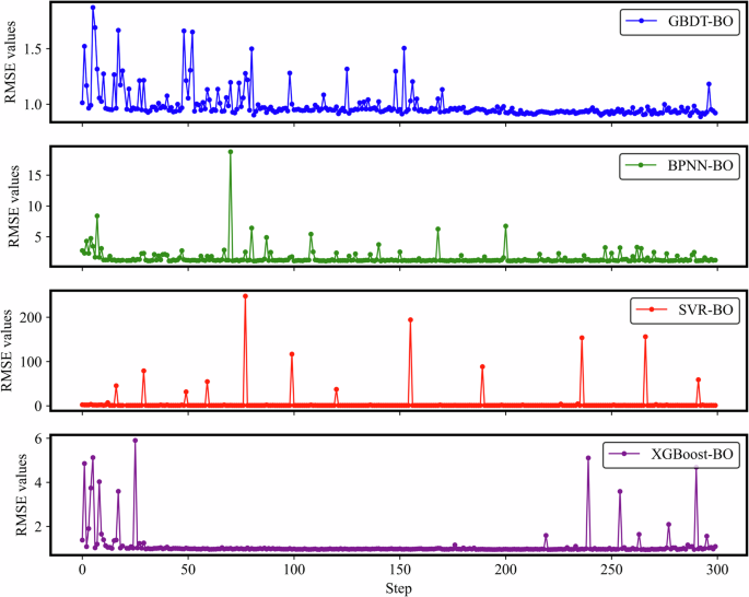
Variations of RMSE for 4 kinds of ML models during the process of Bayesian Optimization.

Full size image

Experimental methods

This experiment refers to the “Test method for the determination of oxidation resistance of steel and superalloy” and the standard indicates that this method can also be used to test the oxidation resistance of titanium alloys. The experiments in this research originally implemented more than 60 Ti-V-Cr alloys production by non-consumable vacuum arc melting and oxidation resistance tests varying the content of V, Cr, and Al. Considering the establishment of machine learning models, the performance of ML models would be compromised by utilizing 60+ groups of data. Hence, the oxidation data and behaviors of high-temperature Ti-alloys such as Ti811, IMI834, and Ti65 were collected, together with the experimental 60+ groups of data (156 samples in total), as the training dataset as well.

Experimental equipment: sample heating furnace, analytical balance, and sample container. The temperature measurement accuracy of the heating furnace is 0.5 °C while the temperature difference in the furnace is less than 5 °C. The average temperature fluctuation in the furnace is less than 3 °C, and the oxidation atmosphere is maintained in the furnace. The accuracy of the analytical balance is 0.0001 g. The container used for the test is a small crucible, and the sample is tilted in the crucible. The contact area between the surface area and the container is kept to a minimum.

During the experiment, the crucible was placed on the tray according to the fixed position. The orientation and the position of the crucible was kept, and the orientation of the tray was marked when taking out the measurement. Before the experiment, the sample was polished flat and left for 1 day. The residue in the crucible was removed and roasted at 650 °C for 5 h, and the quality was measured after being taken out and left for 2 h. Then it was roasted again and taken out to stand and measure the quality. If the difference between the two measurements is not greater than 0.0002 g, it is considered that the crucible has reached constant weight and can be put into the drying chamber for backup. Pallets were roasted in the same way. The experimental temperature was 600 °C while the total experiment time was 100 h and the sample was taken out every 25 h after standing, weighed and then returned to the heating furnace. The experiment was repeated with three samples for each component. The quality of the sample was measured before heating at 25, 50, 75, and 100 h. The oxidation weight gain was calculated, and the oxidation weight gain curve was drawn. Subsequently, the oxidation rate constant was calculated from the oxidation weight gain curve. After the experiment was completed, metallographic samples were prepared by grinding plate method, and metallographic images, scanning electron microscope images and energy spectrum images were obtained by optical microscope and electron microscope.