Assessing the feasibility of using a data-driven corrosion rate model for optimizing dosages of corrosion inhibitors

Corrosion can result in damage to equipment and long downtime in cooling water systems. Corrosion mitigation strategies commonly adopted are maintaining a small scaling deposit on the metal surface, usage of corrosion inhibitors, and treatment of the cooling water to remove corrosive constituents such as chlorides and sulphates^{1,2,3,4,5,6,7,8}. Corrosion inhibitors slow the rates of both cathodic and anodic reactions by reducing the active surface or changing the activation energy of the oxidation or reduction process⁹. The development of corrosion inhibitors and investigation of their inhibition mechanisms have been carried out with the aid of molecular modeling and quantum chemical calculations using density functional theory¹⁰. The latter is based on electron density, which carries information related to atoms and molecules. Investigating micro-mechanisms requires combining first-principles techniques based on fundamental theory, such as the density functional theory with molecular dynamics, peridynamic theory and finite-element methods¹⁰. Although these methods provide comprehensive information about the system under consideration, they are highly computationally intensive. However, their prevailing interest in the field of corrosion is apparent in obtaining insights into micro-mechanisms and interactions among components in a water matrix and the metal surface.

The addition of more than one corrosion inhibitor in cooling systems is commonly applied with the hope of synergistic effects among inhibitor compounds improving the overall inhibition efficiency. Studies have demonstrated the synergism of Zn²⁺ ions with organic corrosion inhibitors¹¹. Synergism between corrosion inhibitors has been investigated using electrochemical impedance spectroscopy by Marin-Cruz et al.⁸ and Touir et al.⁵ in cooling water systems. However, antagonistic effects among inhibitors have also been shown when water qualities change¹². Thus, the inhibitive effectiveness of corrosion inhibitors depends on complex interactions between background ions and other inhibitors^{2,3,4,5,11,12}, as well as the metal under test⁶. These effects are very difficult to predict a priori. Therefore, the determination of corrosion rates, as well as inhibition efficiency in real-life aqueous environments, is commonly done via pilot tests and time-consuming and costly experiments (e.g. using electrochemical impedance spectroscopy)^7,8.

Model development is an alternative method for capturing the synergism among multiple corrosion inhibitors and ions present in the system. Research reported on modeling corrosion inhibition using data-driven models has focused on predicting an aspect related to inhibitors, such as the inhibition efficiency. Corrosion inhibition of mild steel in sulfuric acid has been modeled by Edoziuno et al.¹³. They analyzed corrosion inhibition-related process parameters and their relationships to obtain optimal inhibitor concentration, immersion time, and acid concentration that maximized inhibitor efficiency. Omran et al.¹⁴ conducted a factorial experimental design to maximize the inhibition efficiency in a system of mild steel and water-containing plant extracts. Ansari et al.¹⁵ optimized the interactive effects of temperature, the concentration of inhibitor and immersion time for a maximum response of inhibition efficiency using the Response Surface Method (RSM) in a C38 steel/H₂SO₄ solution. Commercial software such as French-Creek models¹⁶ can optimize multiple inhibitors, but only sequentially. For instance, Ferguson et al.¹⁶ demonstrate how the orthophosphate dosage is first optimized, and subsequently, the copolymer dosage is optimized. These studies have specifically measured the corrosion inhibition efficiency and modeled it with respect to concentrations of corrosion inhibitors and ions. Corrosion inhibition efficiency can be measured using complex and time-consuming techniques such as electrochemical impedance spectroscopy and potentiodynamic polarization techniques.

Corrosion rates of cooling water are conveniently measured in large-scale plants using linear polarization resistance (LPR) in an hourly or daily basis. In the meantime, concentrations of several ions are also regularly measured and recorded. It would be advantageous to use these measurements to replace, or at least minimize the use of costly and time-consuming methods such as potentiodynamic polarization techniques for optimizing dosages of corrosion inhibitors. Due to the complexity in the corrosion inhibition process, data-driven models such as neural networks are most appropriate. These models aim to counter the complexity and the time-intensive character of pilot-scale, lab-scale or molecular modelling experiments.

Authors of the current study identify the following essential properties when using a model developed for predicting the corrosion rate for optimizing inhibitor dosages:

• The prediction accuracy of the model should be satisfactory.

• The model should identify the relationship between the corrosion rate and corrosion inhibitors sufficiently.

Data-driven modeling studies carried out in the literature have demonstrated the corrosion rate can be predicted with adequate prediction accuracy. Aghaaminiha et al.¹⁷ developed a random forest model to predict the corrosion rate of mild steel in CO₂ aqueous solutions with the mean squared error ranging from 0.005 to 0.093 as a function of time over 160 hours. Coelho et al.¹⁸ comprehensively compares the prediction accuracies of different types of data-driven models. Machine learning models that have been reported in corrosion literature are kernel-based methods such as support vector regression, back propagation neural network, deep neural network, tree-based models such as random forest, and gradient-boosted decision trees. The study by Coelho et al.¹⁸ reveals that kernel-based methods such as support vector regression have higher prediction accuracy across different corrosion topics. Although these studies have reported high testing performances, the methods employed in dividing the data set into training and test sets for a proper model evaluation were not clearly described. It is important to demonstrate that the model is capable of predicting events ahead of time. Such events can be defined as changes in corrosion rate in response to varying operational and environmental factors. A study by Zhi et al.¹⁹ demonstrates the difficulty of predicting corrosion rates in diverse conditions.

The relationship between inhibitors and corrosion rate is not as direct as that between inhibitors and inhibition efficiency. Other factors, such as pH have a higher impact on the corrosion rate than inhibitor dosages. During the training process of a data driven model such as a neural network, the model assigns weights to connections between the input variables and the output. More often than not, the model assigns high weights to a handful of variables while the significance of the remainder is diminished²⁰. Therefore, it is likely that the weights assigned to corrosion inhibitors is dependent on other variables used as inputs to the model.

The taxonomy of variable selection for model development has been discussed in several studies^20,21,22. Selection methods are most commonly classified into linear and nonlinear filter, wrapper, and embedded methods. Studies have been carried out to identify suitable variable selection methodologies per field of study^23,24. A comparison of how commonly used variable selection methods affect the corrosion rate prediction accuracy and the significance assigned to corrosion inhibitors has not been carried out to the best of the authors’ knowledge.

Therefore, the current study investigates the feasibility of reliably developing and using a data-driven model trained to predict the corrosion rate for optimizing multiple corrosion inhibitors simultaneously. In view of the stated gaps noted in the literature and challenges experienced when developing a predictive model for corrosion using cooling water data sets, the current study investigates the impact of common variable selection methods on the prediction accuracy of corrosion rate and sensitivity of corrosion inhibitors to the predicted corrosion rate.

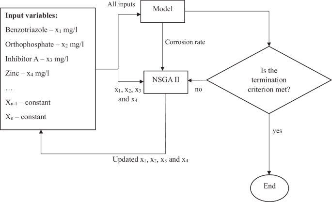
Figure 1 presents an overview of the methodology followed for demonstrating how combinations of input variables affect the prediction accuracy of corrosion rate as well as the significance assigned by the model to corrosion inhibitors. The software used in this study are mentioned in Supplementary Table 1.

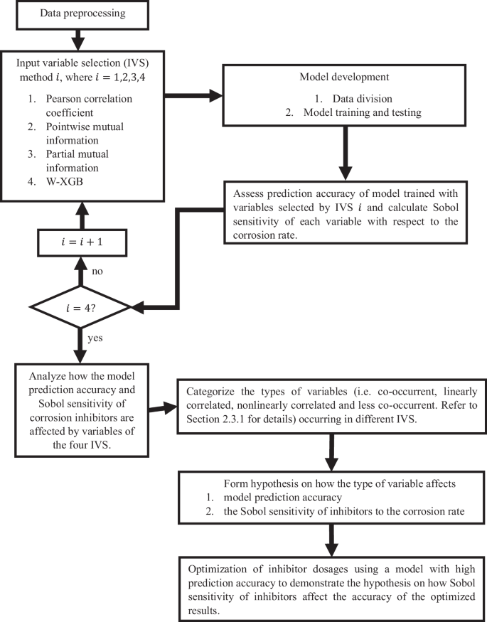
An overview of how input variable selection methods were used to assess the feasibility of optimizing inhibitor dosages.

Full size image

Data set

A data set containing daily measurements of water qualities, chemical concentrations, and corrosion rates (mm/year) of mild steel pertaining to the years 2020 to 2023 was obtained from a cooling water circuit of a chemical plant. The corrosion rates were measured using a mild steel LPR probe (linear polarization resistance) embedded in an epoxy resin (to minimize crevice corrosion) inserted into the piping of a cooling water circuit. The sensor is mounted horizontally in the side branch of a tee, with the flow entering the tee through the top branch and flowing away from the base of the sensor, towards the tips of the electrodes.

Hourly corrosion rates were recorded. As only daily concentrations of ions and inhibitors were available, the corrosion rates were averaged to daily values. Variables available in the data set are shown in Table 1. All variables in Table 1 were not used for model development. Value ranges of each variable shown in Table 1 are given in Supplementary Table 2.

The mean, standard deviation, median, coefficient of variation, skewness and kurtosis of each variable shown in Table 1 is given in Supplementary Table 3. Physical properties and concentrations in the data set had been maintained between practical limits throughout 3 years. Among the corrosion inhibitors analysed in this study, benzotriazole has the highest coefficient of variation (0.38). A kurtosis of 3.26 indicates that the standard deviation is due to frequent modestly sized deviations. Lowest coefficients of variations among the inhibitors can be observed in inhibitor A and orthophosphate (0.1 and 0.12, respectively). However, their coefficient of variation is similar to that of CWFR (0.11). The higher kurtoses of orthophosphate (5.7) and zinc (7.04) indicate that most of their values are closer to the mean. The coefficient of variation of zinc (0.24) is higher than inhibitor A, orthophosphate and CWFR. The correlation coefficients and the p-values for testing the hypothesis that there is no relationship between the variables and the corrosion rate (null hypothesis) are mentioned in Supplementary Table 4. The relationship between the corrosion rate and the variables are nonlinear as the corrosion process is a complex phenomenon. Therefore, the values of the correlation coefficients are low. However, as evident in Supplementary Table 4, the low p values of the variables indicate that the null hypothesis (that no relationship exists between the corrosion rate and the variables) can be rejected. Therefore, the data is suitable for model development.

All variables shown in Table 1 affect the corrosion rate. Orthophosphate is a widely known corrosion inhibitor²⁵. Benzotriazole is commonly used to mitigate corrosion of copper²⁶. However, it has also been proven effective for mild steel²⁷. Inhibitor A is a proprietary chemical tailored to minimize corrosion. Zinc acts as a cathodic corrosion inhibitor by forming complexes with hydroxide ions and precipitating on metal surfaces²⁸. Phosphates and phosphorous based compounds provide anodic as well as cathodic protection to metals^29,30. However, phosphorous-based compounds and TOC could contribute to microbial corrosion³¹. Microbial corrosion is an unavoidable phenomenon in cooling systems³². Therefore, the bacterial count is as an important factor affecting corrosion rate. Ca²⁺ and Mg²⁺ contribute to scaling deposits that often act as a protective covering preventing corrosion of metal surfaces³³. Therefore, antiscalants that are added to regulate scaling deposits affect corrosion. Minute amounts of copper dispensed from copper-containing parts of the cooling system could plate on steel surfaces and induce rapid galvanic effect on them as the distance between steel and copper is high in the galvanic series³⁴. Effect of Nitrate ions on corrosion varies depending on water chemistry, type of metal and physical parameters such as temperature. Nitrates could aggravate corrosion through adsorption and reduction to ammonium^35,36 while also reducing the chances of corrosion by passivation³⁷. Halogenated organic compounds (AOX) are harmful to the environment. The addition of benzotriazole contributes to the AOX concentration²⁶. Variables such as free chlorine, chloride ions, pH, conductivity and temperature are widely known to affect corrosion.

In addition to variables shown in Table 1, historical values of benzotriazole, inhibitor A, orthophosphate, zinc, and flow rate were also considered. Historical values refer to values of a variable from a previous time period. For example, zinc(t-1) refers to the zinc concentration from a day prior to the considered day. Historical values of the corrosion rate were not considered in the first part of this study, as the significantly higher sensitivity of historical corrosion rates makes it difficult to assess the diminished impact of other variables on the predicted corrosion rate. However, they are considered when the final model is presented with an example-result on how inhibitors are optimized at the end of this study. Historical values for inhibitors (i.e. benzotriazole, inhibitor A, orthophosphate and zinc) are considered up to three days (i.e. t-1, t-2, t-3). Those of CWFR was considered up to 4 days as the corrosion rate was visually highly correlated to CWFR, as shown in Fig. 2. It is assumed that high flow rates contribute to greater shearing of the corrosion fouling layer³⁷. As the development of the corrosion fouling layer is time-dependent, longer historical CWFR could be relevant to the prediction of the corrosion rate.

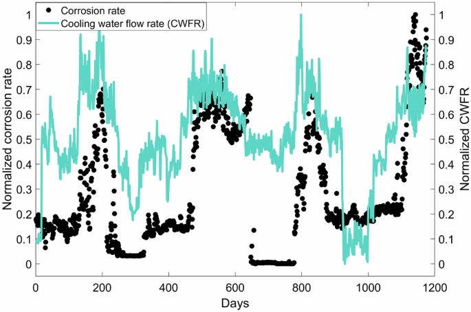
Filled black circles represent measured corrosion rate over time. The light blue-green continuous line represents the corresponding cooling water flow rate maintained in the circuit.

Full size image

Data preprocessing

All variables were normalized between 0 and 1 using Eq. 1 as

Outlier removal was carried out using a method known as the ‘local outlier factor’ (LOF). This method is based on computing the local density deviation of a given data point with respect to its neighbors and was implemented using the sci-kit learn python library³⁸. The LOF method was found to be superior to Z-score method. The Z-score method is highly reliant on the mean of the data. As pointed out by May et al.²⁰, the mean will be affected if a large number of outliers is present in the data set.

Variable selection

Five variable selection methodologies were applied in this study.

1. 1.

   Pearson correlation coefficient (PCC)

   PCC is determined by

   $${rm{PCC}}=frac{sum left({x}_{i}-bar{x}right)left({y}_{i}-bar{y}right)}{sqrt{sum {left({x}_{i}-bar{x}right)}^{2}sum {left({y}_{i}-bar{y}right)}^{2}}}$$

   (2)

   where, ({x}_{i}) and ({y}_{i}) are i^th input vector and output value in the sample; (bar{x}) and (bar{y}) mean values of x and y.

   PCC is a popular linear method of examining the correlation between two variables. The magnitude of the correlation suggests the degree of the linear correlation existing between two variables, while the sign of the value obtained suggests whether the variable is enhancing or inhibiting to its counterpart.

2. 2.

   Point-wise mutual information (point-wise MI)

   Point-wise MI is determined by

   $${rm{Point}}-{rm{wiseMI}}left(x,yright)=log frac{Pleft(x,yright)}{Pleft(xright)Pleft(yright)},$$

   (3)

   where (Pleft(x,yright)) is the joint probability distribution of x (an input variable) and y (the output variable). Reader is referred to May et al.³⁹ for further details on point-wise mutual information. A Gaussian kernel was used to estimate the probability distributions. MI is a nonlinear filter used to quantify the correlation between two variables. Variables with high positive pointwise MI values are ranked high.

3. 3.

   Partial mutual information (Partial MI)

   Partial MI uses the same concept as mutual information; however, it enables the reduction in uncertainty in predicting the output while quantifying the additional mutual observation gained by adding another variable (Z) into a set of already established variables (X). The algorithm employed for implementing partial MI is shown in Supplementary Figure 1. Further details of the partial MI algorithm have been presented by May et al.³⁹. The last step of the algorithm involves selecting a variable that maximizes the pointwise mutual information (({rm{I}}left({rm{v;u}}right))). It was noted that the values of ({rm{I}}left({rm{v;u}}right)) were negative. Therefore, selecting the highest value of ({rm{I}}left({rm{v;u}}right)) could be done as per the magnitude of ({rm{I}}left({rm{v;u}}right)) or based on the more positive value of ({rm{I}}left({rm{v;u}}right)). Thus, partial MI was implemented in two ways¹: positive partial MI – selection of variables giving priority to more positive pointwise mutual information (({rm{I}}left({rm{v;u}}right))) and² magnitude-based partial MI – selection of variables giving priority to the magnitude of pointwise mutual information (({rm{I}}left({rm{v;u}}right))).

4. 4.

   Model-embedded weights-based variable selection using the XGBoost implementation of gradient-boosted decision trees

   XGBoost regression has been successfully used in a multitude of applications including corrosion for prediction and computing feature importance⁴⁰. Feature importances were extracted from an XGBoost model trained with data. The xgboost python package was used for this purpose. Readers are referred to Pedregosa et al.³⁸ for more details of the method.

The methods discussed from 1 to 4 provide a ranking of variables in the order of importance. The selection of the optimal number of variables for model development was done as displayed in Supplementary Figure 2.

Linearly correlated, co-occurrent, and less co-occurrent variables

Three terms are used to categorize variables encountered in this study: linearly correlated, co-occurrent, and less co-occurrent variables. The term ‘linearly correlated’ refers to variables that are considered most relevant by PCC. Co-occurrent variables are considered most relevant by positive point-wise MI. Less co-occurrent variables are high in the magnitude of point-wise mutual information and top-ranked by magnitude-based partial MI, yet not by positive partial MI.

Sensitivity analysis of variables

Sobol sensitivity analysis of input variables was carried out to evaluate the impact corrosion inhibitors had on the predicted corrosion rate. The main purpose of the analysis is to identify how different types of variables affect the Sobol sensitivity of corrosion inhibitors. Most modeling studies that had been carried out on optimizing corrosion inhibitors had focused on predicting quantities such as corrosion inhibition efficiency^13,14,15, which is a more direct consequence of the inhibitors than the corrosion rate. Therefore, it is important to get a clear understanding of the sensitivity of corrosion inhibitors in a model trained to predict the corrosion rate.

Data division

Definition of the test data set to evaluate the model’s ability to predict future events

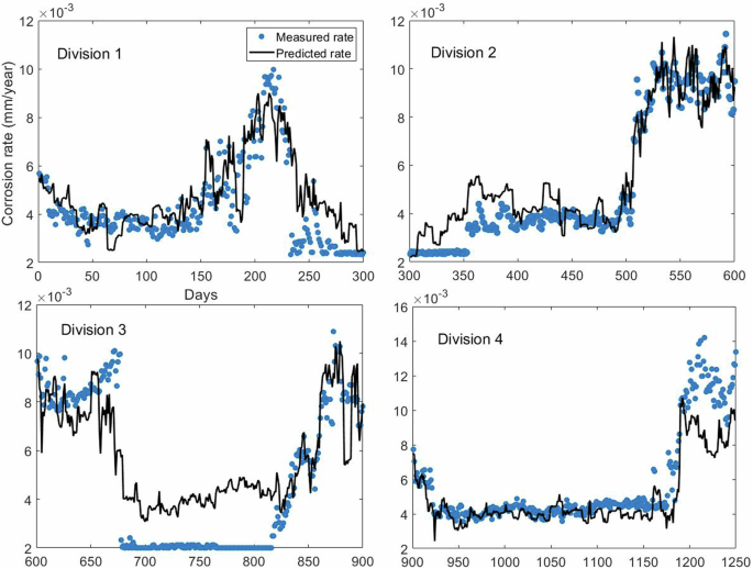
According to a review by Bowden et al.⁴¹, optimal data division for applications in water resources requires ensuring similar statistical properties among training, validation, and test data sets. While paying due consideration to statistical properties warrants adequate training, defining a test data set based on statistical properties does not guarantee that corrosion events will be well predicted. Therefore, cross-validation was carried out by dividing the time-series data, as shown in Fig. 3.

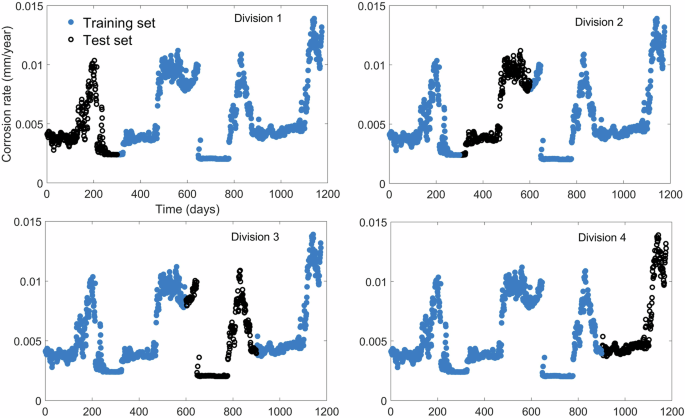
Filled blue circles represent data points allocated to the training data set. Black clear circles represent data points allocated to the test data set.

Full size image

The corrosion profile was divided into divisions of approximately 300 consecutive days where each division defines an event. The model was trained with nearly 900 daily measurements, shown by blue markers in Fig. 3, and tested with the remaining 300 consecutive daily measurements represented by the black continuous line in Fig. 3. For example, when the first 300 data points were defined as the test data set, the remaining 900 were used for training. Thus, a total of four models were trained, one per each division using data points represented by filled blue circles. Each model was tested with data points indicated by black clear circles.

The corrosion profile shown in Fig. 3 pertains to 4 years of data. Periodical increases in corrosion rate noted in Fig. 3 correspond to summer months when the cooling water flow rate is increased to meet the required cooling capacity. As the temperature of cooling water, which is generally drawn from a nearby water body, is high during summer, CWFR is increased to enhance the circuit’s heat capacity. As previously mentioned, increasing the flow rate may result in the shearing of the barrier layer between the metal surface and the bulk fluid. As the barrier layer is formed by inhibitors and corrosion fouling deposits, the removal of the barrier layer enables easier access for corrosive ions towards the metal surface.

The events denoted by the four divisions of Fig. 3 are unique. The test data set of Division 1 demonstrates corrosion rates well within the total range of the data set without any special occurrences. Division 2 represents corrosion rates that are influenced by the occurrence of filtered substances, likely due to an operational event that was only noted in this time period. Division 3 consists of lowest corrosion rates available in the data set. Division 4 consists of highest corrosion rates available in the data set. Therefore, the model’s generalization ability, extrapolation ability and its capability of handling responses to operational changes are tested through the division shown in Fig. 3.

Data division in input variable selection

Input variable selection was carried out using the entire data set. Training and test data sets used for input variable selection were defined based on statistical properties, i.e. the mean and the standard deviation of the training data set were made to be approximately equal to those of the test data set⁴¹. Such an equitable distribution was ensured by first condensing all variables to one variable using principal component analysis and it was used to generate a normal distribution curve as shown in Fig. 4. The distribution curve was partitioned into sections of constant width (e.g. (w=)0.1) where two consecutive partitions were allocated to the training data set and the third consecutive partition was allocated to the test data set. The process was repeated from the negative-most Z-score to the positive-most Z-score.

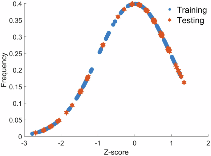
Blue circles represent data points allocated to the training data set. Orange stars represent data points allocated to the test data set.

Full size image

The Z-score was computed as

where (mu) is the mean and (sigma) the standard deviation of the data set.

The width (w) is varied from 0.1 to 0.4 at intervals of 0.1, and the algorithm in Fig. 4 is repeated each time. The width (w) is changed to make sure that the performance of the selected variables remains high through varied apportioning of data points in the test data set in an informed manner.

Support vector regression

As per a comprehensive review on the use of machine learning in corrosion by Coelho et al.¹⁸, support vector regression has demonstrated high generalization ability and prediction accuracy across several corrosion topics.

The mathematical model of SVR is given by Eq. 5.

where ‘k’ is the number of support vectors; (alpha), ({alpha }^{* })– Lagrange multipliers; ({x}_{i}) – input vector of support vector; b – bias; (x) – input vector; y – output, (Kleft({x}_{i},xright)) is the kernel, for which the radial basis function was used.

More information on the support vector regression model can be read in Welling⁴².

Parameters that need to be tuned in a SVR are the box constraint (C, which was set to 1), error sensitivity parameter (ε, set to 0.005) and the smoothing parameter of the radial basis function (γ, set to 0.7). Values of the parameters were determined using a global exhaustive search method.

Optimization

The purpose of presenting the results of optimization in this paper is to demonstrate the implications of using a data-driven model that assigns low weight and sensitivity to optimization. Other aspects of optimization are not within the scope of this study. In order to ensure high prediction accuracy, historical values of the corrosion rate up to 7 days (i.e. CR(t-7)) was used as an input variable. Therefore, in practice, the model developed can only be used for optimizing dosages of the following 7 days. The reason for choosing a week’s time for the historical values of corrosion is to ensure that all allowances are made for the response time required for a change in the inhibitor dosage to take effect. The remaining variables required for developing the model used in this section were selected using the most effective input variable selection method out of Section Variable selection. The inhibitors (i.e. benzotriazole, orthophosphate, zinc and inhibitor A) were also included as input variables.

The NSGA II evolutionary algorithm⁴³ was used for optimization of inhibitor dosages. NSGA II facilitates multi-objective optimization with faster convergence and evaluation of solutions over a larger search space than methods such as gradient descent or particle swarm optimization. The method of optimizing inhibitor dosages using NSGA II is demonstrated in Fig. 5. It should be noted that the inhibitors were varied to determine the optimum values per data point while the remaining input variables of the SVR were fixed as constants (at recorded values), per data point.

Concentrations of benzotriazole, orthophosphate, inhibitor A and zinc are varied such that the required dosages of inhibitors are minimized, while maintaining the corrosion rate at a minimum possible value. The termination criterion used in this study is the number of iterations of the algorithm.

Full size image

The objective functions were defined as stated in Eq. 6

Equation 6 represents two objective functions. The first objective function ({f}_{1}) demonstrates how the concentrations of the inhibitors are weighted. Benzotriazole is weighted higher than the remaining inhibitors. Therefore, the NSGA II algorithm gives higher priority to reducing the concentration of benzotriazole over others, due to its harmful environmental impact. In the meantime, the algorithm also minimizes the corrosion rate that is resultant from minimized concentrations of inhibitors. The constraints imposed on this algorithm are that the concentrations of the inhibitors are always maintained between the minimum and maximum values in the available data set.

Variable selection

The current section presents results of variables selected for model development by the four input variable selection methods discussed in Section Variable selection. The variables are listed in the descending order of importance as specified by each method. The number of variables per method was selected according to the algorithm shown in Supplementary Figure 2. The results obtained are presented in Table 2.

A similarity can be noted among the variables chosen by PCC, positive point-wise MI, and positive partial MI. W-XGB ranks variables based on the overall weights assigned by a trained XGBoost implementation of gradient boosted decision trees to each variable. Therefore, the method captures the phenomenological relationship between the corrosion rate and the input variables than PCC, pointwise MI or partial MI. Therefore, W-XGB identifies the importance of nonlinear and less co-occurrent variables such as Nitrate. Partial MI enables identifying variables that further reduce the uncertainty surrounding the corrosion rate that is gained by the additional mutual observation of a variable³⁹. Therefore, variables selected by partial MI complement the information already embedded in the first set of variables. The first set of variables were set as corrosion inhibitors in the system. Thus, the remainder of the variables are expected to complement the information embedded in the data pertaining to the inhibitors. As noted in Table 2, CWFR is considered an important variable by all variable selection methods. Additionally, the variable named filtered substances is considered important by all methods shown in Table 2, even though it corresponds to a one-time event that occurred in Division 2 of Fig. 3. W-XGB recognizes N-containing compounds as well as historical values of Inhibitor A and orthophosphate as important variables as opposed to PCC, point-wise MI, and partial MI.

Test results from predicting events demonstrated in Fig. 3 using the trained SVR with input variables in Table 2 are illustrated in Supplementary Figs. 3 to 6. The models developed by all variable selection methods have predicted the rate of corrosion in Division 1 with reasonable accuracy. PCC and MI have best predicted the corrosion rate in Division 2. None of the models were able to successfully extrapolate less than the minimum corrosion rate or higher than the maximum corrosion rate in the training data set, as evident from the predicted corrosion profiles in divisions 3 and 4. The minimum corrosion rate occurs in Division 3, while the maximum corrosion rate occurs in Division 4.

As stated in Section on Variable selection in the Methodology, partial MI in Table 2 was implemented such that variables with high positive point-wise mutual information were given priority. Positive point-wise MI suggests that variables co-occur with the output, i.e. variables that respond at the same time as corrosion with a high probability. According to Table 2, there is a significant similarity among variables selected by partial MI and PCC. It appears that the most linearly correlated variables are similar to the most co-occurrent variables. However, variables with negative point-wise MI cannot be deemed irrelevant as only a value close to 0 is considered irrelevant⁴⁴.

Partial MI determines water quality measurements that support the prediction of the corrosion rate, in addition to the starting fixed set of pre-determined variables (i.e. benzotriazole, orthophosphate, inhibitor A, and zinc). In doing so, most variables were noted to have high negative point-wise MI. High negative point-wise information indicates that a variable does not co-occur well with the output variable. In other words, such a feature is of a probability distribution complementary to that of the output variable. A comparison of features selected by magnitude-based partial MI and positive partial MI, as well as magnitude-based point-wise MI and positive point-wise MI is given in Table 3. Nitrate was ignored from variables under magnitude-based point-wise MI as it is highly correlated to TIN. Similarly, HCO₃^– was ignored as it is highly correlated to TIC.

Variables selected by magnitude-based partial MI shown in Table 3 include those that co-occurs less with the corrosion rate, such as organic phosphorous, total phosphate, and AOX. KS4.3, HCO₃⁻, inhibitor A (t-1) and TIC are common with magnitude-based partial MI and W-XGB. The main difference between the sets of variables selected by positive point-wise MI and magnitude-based point-wise MI is that the latter identifies nitrates and TIN as important variables. As observed in Table 2, Nitrate is also identified as important by W-XGB. As W-XGB is capable of identifying nonlinear variables that significantly affect corrosion, it appears that magnitude-based partial MI ensures the inclusion of variables that are non-linearly correlated and less co-occurrent with the corrosion rate. However, due to the lack of linearly correlated/co-occurrent variables among magnitude-based partial MI variables, the prediction accuracy has declined, as shown in Supplementary Table 5.

None of the variables selected by magnitude-based partial MI are sufficiently co-occurrent and/or linearly correlated to the corrosion rate. Therefore, the prediction accuracy of a model trained with these variables is not adequate. In order to facilitate predicting the corrosion rate using data-driven models, the presence of one or more co-occurrent/linearly correlated variables seem essential. This was demonstrated by the addition of two co-occurrent variables: CWFR and [Ca²⁺]. As shown in Fig. 2, CWFR is highly correlated to the corrosion rate. As scaling contributes to the formation of a barrier layer between the metal surface and the solution, Ca²⁺ ions contribute to the inhibition of the corrosion rate. Ca²⁺ concentration has also been listed as a highly linearly correlated variable under PCC in Table 2. Therefore, CWFR and Ca²⁺ were included among the top-ranked variables along with benzotriazole, inhibitor A, orthophosphate and zinc. The remaining variables were selected by re-implementing the partial MI algorithm in May et al. (2008). The number of variables was determined with the algorithm shown in Supplementary Figure 2. The variables resulting from repeating the magnitude-based partial MI algorithm were Ca²⁺, CWFR, benzotriazole, inhibitor A, orthophosphate, zinc, COD, AOX, zinc(t-1), total phosphate, zinc(t-3), zinc(t-2), and organic phosphates. A comparison of prediction accuracies of models trained with positive partial MI, magnitude-based partial MI and the latter with Ca²⁺ and CWFR is given in Supplementary Table 6. It can be observed that the addition of linearly correlated and co-occurrent variables improved the predictive ability of the model trained with magnitude-based partial MI variables.

Sensitivity analysis

Sobol sensitivity analysis⁴⁵ was carried out based on SVR models developed using input variables selected by PCC and magnitude-based partial MI by calculating first-order and total Sobol indices. The purpose of the analysis is to understand the difference between the impact of linearly and nonlinearly correlated variables on the sensitivity of inhibitors. Dissolved zinc was omitted as a variable for model comparison as it is correlated to the total amount of zinc. Filtered substances was also omitted as a variable, as its values correspond to a single operational change. The main objective of the model is to optimize dosages of benzotriazole, inhibitor A, orthophosphate and zinc. Therefore, including variables highly correlated to the four inhibitors will provide redundant information and inconvenience optimization of the inhibitors from having to account for the correlations with the input variables. Orthophosphate and inhibitor A are slightly correlated to total phosphates. However, the model prediction accuracy demonstrated in Figs. A3 to A6 are also not perfect. In the meantime, total phosphates are highly influenced by antiscalants added to cooling water. As antiscalants are not accounted for by the variables included in this study, total phosphates were not excluded. The results of the Sobol sensitivity analysis are given in Table 4.

When comparing 1^st order Sobol sensitivities of magnitude-based partial MI with and without CWFR and Ca²⁺, the relative sensitivities assigned to corrosion inhibitors, especially benzotriazole, decline notably upon the addition of variables more linearly correlated to the corrosion rate. As observed in Fig. 6, the Sobol sensitivity of zinc is low in both instances when magnitude-based partial MI was used. Based on Table 4, historical values of zinc appear to have a higher influence on the corrosion rate than the present value. Among variables considered by PCC pH, benzotriazole and CWFR, have the highest 1^st order Sobol indices. Therefore, they have the highest sensitivity to corrosion rate.

Total Sobol index is an overall sensitivity accounting for sensitivity of a variable to the output as well as interaction effects among other variables. The highest total Sobol indices of PCC variables can be observed in pH, benzotriazole, and zinc.

The 1^st-order Sobol sensitivity of benzotriazole among magnitude-based partial MI (without CWFR and Ca²⁺) and PCC variables are similar. The sensitivity of benzotriazole is low when the model is trained with partial MI variables with CWFR and Ca²⁺. Therefore, unique combinations of variables have an impact on the Sobol sensitivity of an inhibitor. It appears that linearly correlated and co-occurrent variables are suitable for predicting trends of corrosion rate, whereas, magnitude-based partial MI variables ensure a high Sobol sensitivity of corrosion inhibitors to the corrosion rate.

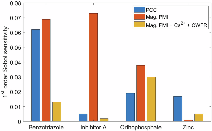
The 1^st order Sobol sensitivity of benzotriazole, inhibitor A and orthophosphate are highest among variables chosen by magnitude-based partial MI. The decline in the sensitivity of zinc is due to zinc (t-2) and zinc(t-3) being correlated to zinc, which have higher sensitivities as presented in Table 4.

Full size image

Optimization

Model prediction accuracy and sensitivity to corrosion inhibitors were considered vital for optimization of corrosion inhibitors in this study. Although PCC variables demonstrated the highest prediction accuracy, it is apparent from Supplementary Fig. 6 that the predictions largely fluctuate from the measured rates. Therefore, historical values of corrosion rate were included as an input variable. As described in Section on Optimization in the Methodology, the historical value of the corrosion rate 7 days prior to the considered time ‘t’, CR (t-7), were used as historical values. The remainder of the input variables (in addition to the inhibitors) were selected using PCC. Variables used for model development are benzotriazole, inhibitor A, orthophosphate, zinc, CR (t-7), CWFR, CWFR (t-7) and benzotriazole (t-7). Sobol sensitivity indices with respect to the variables are given in Table 5.

It is clear from Table 5 that the sensitivity of CR(t-7) is significantly higher than other variables. The Sobol sensitivities of benzotriazole, inhibitor A, orthophosphate and zinc are notably lower than the Sobol sensitivity of CR(t-7). Prediction of events indicated in Fig. 3 is shown in Fig. 7.

Model prediction accuracy for the four divisions shown in Fig. 3 The R² and RMSE of the predictions of the four divisions are given in Table 6.

Full size image

A significant improvement of the prediction accuracy can be observed upon the addition of CR(t-7) as a variable. In order to demonstrate how model structure affects prediction accuracy as well as Sobol sensitivities of inhibitors, the SVR was compared with two other models that have frequently demonstrated high predictive performance in the corrosion literature: XGBoost implementation of gradient based decision trees (XGB) and Gaussian process regression (GPR). Apart from the fact that they are all regression models SVR, GPR and XGB differ from each other. SVR is deterministic (each input always provides the same output), GPR is probabilistic based on Bayesian inference (provides a distribution over functions that fit the data) with uncertainty quantification. GPR is non-parametric with complexity adapting to the data while SVR is parametric and assumes a specific form of the function it fits (e.g., polynomial). XGB builds an ensemble of decision trees sequentially, where each new tree corrects errors made by the previous trees, while SVR uses mathematical optimisation to try and find the hyperplane that best fits the data (with kernel functions to deal with non-linearity in the data). Input variables indicated in Table 5 were used for the model comparison. As demonstrated in Supplementary Figure 7, the prediction accuracies of GPR and XGB are similar to SVR. As shown in Supplementary Table 7, Sobol sensitivity analysis reveals that GPR and XGB models also assign the highest sensitivity to the most linearly correlated variable (CR(t-7)).

The model was used to optimize inhibitor dosages and minimize the corrosion rate as described in the section on Optimization under the Methodology. It should be noted that the inhibitors were varied to determine the optimum values per data point while the remaining input variables of the SVR shown in Table 3 were fixed as constants (at recorded values), per data point.

According to Fig. 8 the optimized concentrations of benzotriazole is set to nearly zero throughout the entire time period. Optimized concentrations of orthophosphate, inhibitor A and zinc are also set to minimum values for 1100 days. However, the optimized corrosion rate follows the trend of measured rates despite the significant decreases in the inhibitor concentrations. The model appears to depend on CR(t-7), which is the most linearly correlated to the corrosion rate, to make predictions. The lack of sensitivity to inhibitors has resulted in the model barely accounting for the large decreases in inhibitor dosages.

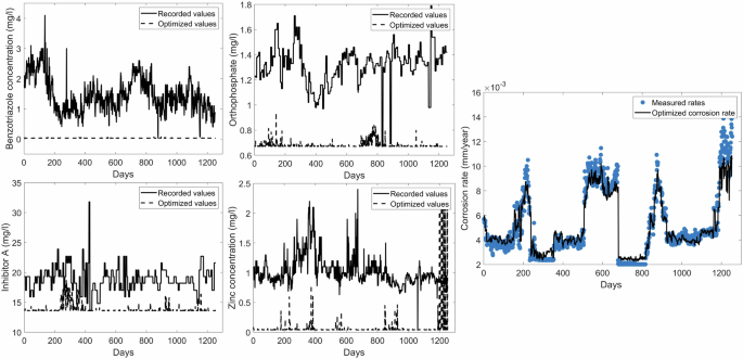
Figure 8 demonstrates how the corrosion rate responds to the optimized concentrations of benzotriazole, inhibitor A, orthophosphate and zinc.

Full size image

The optimized corrosion rate is slightly higher than measured rates at low corrosion rates. The increase in corrosion rate in response to decreases in inhibitor dosages can be expected. The optimized corrosion rates appear to be less than measured rates at high corrosion rates. However, the inhibitor concentration transported to the surface of the metal decreases as the inhibitor dosages decreases as drastically as shown in Fig. 8. This should result in an increase in the corrosion rate. Studies carried out by Barmatov et al.⁴⁶ and Khan et al.⁴⁷ demonstrate how the corrosion rate increases when the inhibitor dosages are decreased at high flow rates.

Therefore, regardless of the high prediction accuracy, inhibitors cannot be optimized using a data-driven model if it overlooks the impact of inhibitors by assigning insignificant Sobol sensitivities. It is apparent that in any data-driven model trained to improve the prediction accuracy of the corrosion rate, linearly correlated or co-occurrent variables are given the highest priority.

As discussed in the Section on Variable selection in the Methodology, variables selected using magnitude-based partial mutual information give higher priority to inhibitors. The shortcoming of magnitude-based partial mutual information was that the model prediction accuracy was not sufficient. However, it is possible to use deep neural networks (DNNs) for improving the prediction accuracy of corrosion rate based on these variables. Although, DNNs can capture nonlinearities well, they are extremely data-hungry models. Therefore, the only remaining alternative is to integrate mechanistic aspects of corrosion with a data-driven component. As corrosion is a complex process involving several reactions, it is not possible to rely on a mechanistic model alone. Therefore, a combination of mechanistic as well as data-driven, also known as a hybrid modelling approach must be employed to facilitate optimizing inhibitor dosages.