XGBoost model for the quantitative assessment of stress corrosion cracking

Corrosion phenomena are of significant concern in modern industry, given their profound environmental and economic implications¹. For instance, recent studies project that by 2030, carbon dioxide (CO₂) emissions from steel replacement due to corrosion could represent up to 9.1% of worldwide emissions, challenging efforts to meet international climate targets^2,3. From an economic standpoint, corrosion’s impact is equally substantial. A consensus exists that the financial ramifications of corrosion may account for 3–5% of a nation’s annual gross domestic product (GDP), approximating $2.2–$2.5 trillion annually^4,5. However, these figures reflect only direct costs in preventive measures and corrosion management⁶. Other indirect costs, such as productivity losses, damage payouts, and environmental impacts, lack a standardised measurement framework^2,4. Nonetheless, it is hypothesised that indirect costs attributable to corrosion could be on par with direct ones; consequently, the cumulative economic impact of corrosion might surpass 6.2% of the global GDP^4,7.

As a result, considerable research has emphasised the importance of mitigating heinous forms of corrosion, principally stress corrosion cracking (SCC)^8,9,10. It is a type of environmentally assisted cracking (EAC), responsible for the catastrophic fracture of materials due to the synergistic interaction between mechanical loads, external, residual or both, and an aggressive environment¹¹. Stress corrosion cracking is pervasive and leads to premature failures of structural alloys used in various industrial sectors, including oil and gas, nuclear power, nuclear waste storage, and aerospace¹².

Among the many strategies to prevent SCC, the selection of corrosion-resistant alloys (CRAs) is often the preferred approach to ensuring the service life of materials across a wide range of severe environments^13,14. Fundamentally, CRAs are engineered to exhibit reduced corrosion rates—when compared to carbon steel—by promoting the formation of protective passive surface films^14,15. The protective passive layer minimises the susceptibility to localised corrosion attacks (i.e., pitting, crevice, and intergranular corrosion), which are precursors to various EAC mechanisms, including SCC, certain forms of hydrogen embrittlement (HE), and corrosion fatigue (CF)¹⁶. Despite their advantages, CRAs can still be susceptible to SCC under specific stress-environment-metallurgical state combinations. Meanwhile, much debate remains regarding the underlying SCC mechanisms and how metallurgical conditions (e.g., composition and microstructure) influence SCC resistance^15,17.

The development of CRAs has largely been unfolded through trial-and-error, aided by laboratory testing and field experience¹⁴. Thus far, the prevalent methodology in metallurgical alloy design consists of selecting a primary component to meet specific property requirements, while conferring secondary properties with a variety of alloying additions, thermomechanical processing, and heat treatments¹⁵. Following this approach, several investigations have provided insights into diverse alloy systems resistant to SCC^{17,18,19,20,21,22}. Consequently, a broad spectrum of multicomponent alloys has been developed and commercialised, centred around a main component, and integrating diverse alloying constituents to achieve the desired balance of in-service properties²³.

In examining the design of CRAs, it is essential to understand the specific roles and contributions of the alloying elements involved. For example, stainless steel (SS) alloys are primarily based on iron (Fe) on account of its formability, enabling easy shaping, manufacturing, and cost²⁴. Nickel (Ni) forms the basis of Ni-base alloys due to its high melting point and capability to dissolve elements such as chromium (Cr), molybdenum (Mo), and tungsten (W) without forming secondary phases^25,26. Cr is responsible for the formation of a passive film in both SS and Ni-base alloys, and it is well-known for its effectiveness in oxidising conditions^15,27. Other alloying elements, such as Mo, W, nitrogen (N) and copper (Cu), are added to promote repassivation in chloride-containing solutions, and to enhance corrosion resistance in reducing environments¹⁵. Furthermore, additions of carbon (C), titanium (Ti), and aluminium (Al) can be incorporated to increase overall strength, or to improve high-temperature oxidation resistance²⁵. Nevertheless, the synergies among alloying elements have been empirically inferred, with no comprehensive theoretical framework to assess their interactions and effects on SCC resistance quantitively¹⁴.

Due to its inherent complexity, SCC necessitates a multidimensional research approach. Thus, machine learning (ML) techniques present a promising avenue. These data-driven methods have extensively been employed in computational alloy modelling^28,29. Recent ML applications have facilitated comprehensive analyses of complex corrosion processes, including coupled chemical and electrochemical reactions, solid-state dynamics, and biological interactions^30,31,32,33. An extensive review of ML applications in corrosion engineering has been elegantly detailed by Coehlo et al.³¹

The current study introduces an ML regression model to quantify SCC susceptibility. Emphasis is placed on the complex interactions between alloying elements and the applied stresses contributing to SCC. The dataset utilised compiles the information from the seminal works of Copson³⁴ and Staehle et al.³⁵, encompassing 269 diverse Fe-Cr-Ni alloys tested in boiling magnesium chloride (MgCl₂). Our preceding publication³⁶ thoroughly interrogates these data and their associated SCC failure patterns using unsupervised learning techniques, such as feature extraction and clustering. The present work builds upon and extends the insights derived from the aforementioned ML study.

Since SCC is a multivariate phenomenon, we employ extreme gradient boosting (XGBoost)³⁷, an ensemble learning method renowned for handling highly dimensional data³⁸. Recently, the XGBoost algorithm has effectively predicted corrosion-related parameters across several engineering domains, including the safety assessment of pipelines, steel property optimisation, and structural damage estimation^39,40,41. In this study, our XGBoost regression model evaluates the SCC susceptibility of SS and Ni-base alloys based on tensile toughness (herein denoted as U_T); a fundamental property generally regarded as the amount of energy (or damage) that a material can withstand before fracturing⁴². By leveraging the relationship of U_T with alloy composition and mechanical properties, we investigate SCC resistance as a function of both, the variations in chemical constituents within a given alloy and the applied stress conditions. Ultimately, we employ interpretable artificial intelligence (AI) on the XGBoost regression model to quantitatively determine the impact of alloying features and their interactions. Principally, Shapley additive explanations (SHAP) are exploited to elucidate the contributions of alloying constituents toward SCC resistance.

In the following section, we present an overview pertinent to the present investigation, detailing critical insights into the publications by Copson³⁴ and Staehle et al³⁵.

Relevant Background

Several investigations have focused on modifying the chemical composition of alloys to mitigate SCC^{43,44,45,46,47}. Within this field of study, the influential work by Harry Copson³⁴ in 1959 established the beneficial effect of Ni on increasing SCC resistance. Copson’s methodology involved documenting the failure times of wire samples composed of Fe-Cr-Ni alloys with Ni concentrations ranging from 8 to 77 wt%. These samples were subjected to a 30-day test in a boiling 42% MgCl₂ solution under constant tensile loading. The outcomes of this study have been captured in textbooks as the so-called Copson’s diagram (Fig. 1a), which is used to indicate the onset of immunity to SCC at 45 wt% Ni.

a Original Copson Diagram³⁴. Herein, the colour shows the stress conditions for each specimen. Red depicts samples stressed below 90% ({sigma }_{{YS}}), while blue represents those stressed at 90% ({sigma }_{{YS}}) or above. The samples in this study range from 8 to 77 wt% Ni, 18–20 wt% Cr, with minor inclusions of Si, Mn, Mo, C, N. b Modified Copson Diagram incorporating data from Staehle et al.³⁵ The colour differentiation indicates groups of alloys based on chemical compositions. Group I comprises Fe-Cr-Ni ternary alloys. Group II represents samples with alloy bases of Fe-15Ni-20Cr, Fe-50Ni-5Cr, Fe-76Ni-15Cr, and Fe-45Ni-30Cr, combined with minor additions of elements possessing atomic diameters nearly equivalent to Ni. Group III involves samples with an alloy base of Fe-15Ni-20Cr, and additions of Be, Al, and C. Group IV comprises specimens with 10–15 Cr + 10–20Ni + 0.1–1.25 Be + 0.1–1.25 Al. Group V indicates commercial SS and Ni-base alloys. Adapted from³⁶.

Full size image

However, Copson’s work has been the subject of debate. Upon reviewing the findings from Copson’s research³⁴ by 1959, it was deduced that alloy 600 was the most suitable for industrial applications (chiefly in the power generation sector), as its Ni content surpasses 72 wt%. Nevertheless, the persistent occurrence of SCC in this type of alloy led to a series of debates aimed at validating Copson’s claims. In this regard, the publications by Staehle and Féron^48,49 thoroughly examine the historical context and the impact of Copson’s research comprehensively.

Several studies have presented conflicting evidence regarding the influence of Ni on SCC resistance^{19,20,21,50,51}. A chief example is the investigation by Staehle et al.³⁵, in which the SCC susceptibility of a broad range of Fe-Cr-Ni alloys was examined under experimental conditions analogous to those in Copson’s work. The results of this study demonstrated that alloys with a Ni content exceeding 50 wt% experienced SCC in boiling MgCl₂. Interestingly, it was found that minor additions of Al and beryllium (Be) increased SCC resistance, even in samples containing 5 wt% Ni. Figure 1b shows the results from Staehle et al.³⁵ using the relationship between Ni content and time-to-failure, thereby facilitating a comparative analysis with the results from Copson’s study.

In their seminal investigations, Copson³⁴ and Staehle et al.³⁵, adopted a descriptive approach that focused on the correlation between alloying elements and SCC resistance, as measured by time-to-failure under constant loading conditions. Nonetheless, pertinent aspects of material mechanics, such as strength and ductility, were incompetently addressed. The exclusive focus on chemical composition constrained the exploration of the interrelationships among factors contributing to SCC (i.e., environment, stress, and material).

Recognising such limitations, Rojas et al.³⁶ recently employed advanced ML techniques to re-analyse the data from Copson³⁴ and Staehle et al.³⁵, thereby offering a holistic examination of the metallurgical factors influencing SCC resistance. A key aspect of this study was the application of t-distributed stochastic neighbour embedding (t-SNE) for feature extraction and clustering. Despite the complexity of the high-dimensional dataset, comprising 37 features and 269 data items (refer to Table 1), the t-SNE algorithm facilitated data segmentation into coherent clusters. Remarkably, the alloying systems within each cluster exhibited significant similarities in failure times, chemical composition, and mechanical properties, namely yield strength (({sigma }_{{YS}})), strain at failure (({varepsilon }_{f})), ultimate tensile strength (({sigma }_{{UTS}})), as well as U_T.

After statistical evaluations within each cluster, Rojas et al.³⁶ corroborated the positive contribution of Ni to SCC resistance, albeit it was found to be inconsistent above 45 wt% Ni. This was observed in alloys with Ni content between 20 and 45 wt%, which surpassed 20 days in SCC testing in boiling MgCl₂. Conversely, alloys exceeding 45 wt% Ni failed consistently around the 10-day mark. Furthermore, minor alloying additions such as Si and Mn were detrimental to SCC resistance. In this case, alloys containing between 15 and 40 wt% Ni, and up to 20 wt% Cr, diminished markedly their failure times due to the presence of both Si and Mn. Apart from this, the discrepancies between Copson’s and Staehle et al.’s studies were attributed primarily to variations in stress conditions. Whereas Staehle et al. maintained a consistent approach by loading the samples at 90% of their yield point, Copson used two fixed loads (i.e., 227.5 and 310.3 MPa), resulting in the irregular testing of numerous specimens. As depicted in Fig. 1a, several alloys in Copson’s study were stressed below 90% ({sigma }_{{YS}}).

Rojas et al.³⁶ also indicated that U_T is an important feature in examining SCC resistance. Fundamentally, U_T relates to the area under the stress-strain curve of a specific alloy, encompassing its main mechanical properties (i.e., ({sigma }_{{YS}}), ({varepsilon }_{f}), and ({sigma }_{{UTS}})), which are largely dependent on the chemical composition and processing history. Thus, the authors suggested that U_T was vital in the pattern recognition analysis and the subsequent characterisation of SCC failure rates, as U_T was the most distinctive feature in differentiating each cluster within the data.

In corrosion engineering, U_T is one of the metrics that enables quantifying the susceptibility to SCC in relevant environments. Researchers routinely determine SCC resistance by comparing stress-strain curves, which are often obtained from slow strain rate testings (SSRTs) in both, an inert control environment and specific test solutions⁵². In this regard, SCC results in a notable decrease in mechanical properties compared to the control case. Thus, SCC susceptibility is quantified using well-established formulae of the form⁵³

Hence, an SSRT ratio approximating 1.0 indicates a low susceptibility to SCC under the conditions of interest. In contrast, SSRT ratios significantly below 1.0 suggest poor resistance to SCC. Nevertheless, there is no agreement on a threshold to define an acceptance criterion.

Aside from U_T, other metrics derived from SSRTs are customarily used to evaluate SCC. These include the changes in time-to-failure, maximum load achieved before failure, or elongation at fracture. Alternatively, SCC analyses can be complemented by post-test information, such as the reduction in area, the plastic strain leading to failure, and the segment of the fracture surface indicative of SCC⁵³. Although SSRT-derived data offer insights into SCC resistance, they may not provide a comprehensive understanding of the multiple factors involved in SCC. In fact, the reliability of SRRT information is subjected to interpretations given its dynamic conditions, where the test variables (mainly strain rate) and evaluation criteria are arbitrarily established and based on experience¹¹. Furthermore, inconsistencies can arise in comparative analyses using SSRTs due to issues in achieving repeatability and reproducibility. In this respect, Beavers and Koch⁵⁴ have documented several SCC studies where SRRTs yielded false positives and negatives, showing discrepancies compared to other SCC test methods (e.g., constant load and strain tests) and field observations.

Another frequently employed metric for evaluating the corrosion resistance of CRAs is the pitting resistance equivalent (PRE), given by^55,56

The PRE is used to measure the susceptibility to localised corrosion, which can further lead to SCC. However, PRE is a simplified empirical fitting of experimental data with critical limitations. Taylor et al.¹⁴ highlighted that PRE does not consider the synergistic effects among alloying elements and the influence of various factors, such as microstructure, processing or stress conditions, and environmental variables. Moreover, the PRE model proves inadequate in evaluating CRAs with novel compositions, particularly when these encompass elements besides Cr, Mo, N, and W. Therefore, the authors emphasised the need to develop robust models and metrics grounded in scientific principles and data-driven methodologies. Such models seek to establish how variations in alloying element ratios, along with metallurgical, technological, and mechanical properties, influence localised corrosion and SCC susceptibilities. To address this need, the current study presents a data-driven approach that utilises the XGBoost algorithm to elucidate the impact of alloying elements and their interactions on SCC resistance, with U_T playing a pivotal role in its realisation.

Data Processing

To evaluate susceptibility to SCC, we harness the ratio of U_T to the time-to-failure observed during SCC testings in boiling MgCl_2. This ratio, hereafter denoted as α, serves as the target variable for the XGBoost regression model. The basis of this approach lies in the properties of U_T, which quantifies the energy absorbed per unit volume until rupture occurs⁵⁷. More importantly, U_T integrates the mechanical properties (i.e., ({sigma }_{{YS}}), ({varepsilon }_{f}), and ({sigma }_{{UTS}})) into a single measure, which in turn is fundamentally influenced by the chemical composition. Thus, we conceptualised α as the volumetric rate of energy absorption (in units of kJ m^–3 s^–1), providing a holistic metric that reflects how efficiently alloy systems absorb energy relative to their durability under SCC-inducing conditions.

The time-to-failure data used to calculate α were acquired from SCC tests under constant tensile stresses (see Table 1), specifically adjusted to each sample’s elastic limit. These loadings could therefore be either above or below the respective yield points. Additionally, U_T values were estimated by the Ramberg-Osgood model (see Methods section), using the mechanical properties measured at relevant testing conditions, as reported by Copson³⁴ and Staehle et al.³⁵ Accordingly, α approximates the energy absorption rate of a metallic alloy under sustained tensile stresses, whether above or below the yield point, which gradually leads to failure in a chloride-rich environment.

By using α, the XGBoost regression model is strategically tailored to employ predictors such as the chemical compositions of the samples and a stress state parameter, specifically ({sigma }_{R}) which is the ratio of applied tensile load to yield strength (see Methods section). Thereby, the matrix representation of the XGBoost model adopts the following form

where X is the matrix of predictor variables used for training the XGBoost regression model, ({x}_{i{rm{j}}}) represents the j-th chemical constituent for the i-th sample, and ({sigma }_{{Ri}}) represents the stress state parameter for the i-th sample. Y is the vector of target values for the XGBoost regression model, with ({alpha }_{i}) being the corresponding target value for the i-th sample.

Figure 2 illustrates the behaviour of the energy absorption rate α, as well as its normalised form used for training the XGBoost regression model. Figure 2a depicts the progression of α values from the most to the least SCC-resistant samples. Here, lower α values suggest gradual energy absorption, which correlates with prolonged times in SCC testings with boiling MgCl₂. Conversely, higher α values indicate a rapid energy absorption, resulting in accelerated failures due to SCC. As shown in Fig. 2a, the energy rate α behaves exponentially, introducing a high level of non-linearity. This issue is addressed by normalising α values through the Box-Cox model⁵⁸. It is a parametric power transformation technique that conveniently stabilises the variance in the target variable, allowing the XGBoost algorithm to effectively learn the non-linear relationships between α and the predictive features. Figure 2b illustrates the Box-Cox transformed values of α, which exhibit a more normally distributed and homoscedastic behaviour. Notably, the Box-Cox transformation maintains the ordinal relationship between α and SCC susceptibility, meaning that the highest transformed α values correspond to the highest energy absorption rates in Fig. 2a and, therefore, the lowest resistance to SCC.

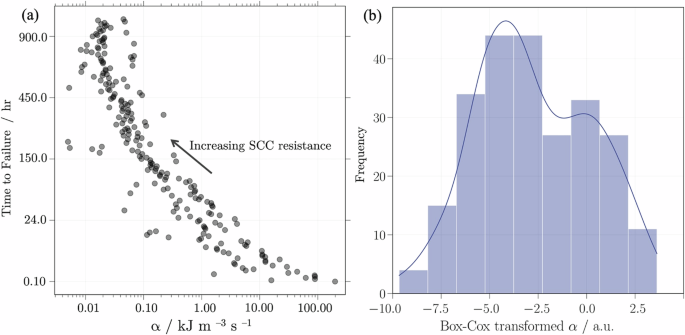
a Energy absorption rate α relative to the time-to-failure in SCC testing in boiling MgCl₂. Here, α indicates the increase in SCC susceptibility, transitioning from the most to the least resilient samples in SCC tests. Therefore, the high α values suggest that the alloys absorb substantial energy from both stress and the environment, leading to accelerated failures by SCC. b Distribution of the Box-Cox-transformed α. The histogram demonstrates the effectiveness of the Box-Cox transformation in normalising the distribution of the target variable. Positive values of the transformed α correlate with the highest energy absorption rates, indicating increased susceptibility to SCC.

Full size image

Given the high dimensionality of the dataset, conventional outlier detection was not feasible. Instead, we implemented a filtering strategy that removed 49 specimens to maintain consistency in the training dataset and prevent bias in the model’s performance. For model training, therefore, specimens subjected to stress conditions exceeding 50% ({sigma }_{{YS}}) were selected from the compiled dataset. As observed by Denhard⁴⁷, alloys under very low tensile stress tend to sharply increase the failure time in SCC tests. Such conditions may outweigh the impact of chemical composition, which in turn bias the XGBoost training. Furthermore, hardened samples from Copson’s study³⁴, possessing a very low ductility (({varepsilon }_{f}le 5 %)), were excluded to ensure that the XGBoost model is trained with data points whose SCC failure behaviour is not unduly affected by hardening processes.

Feature selection

Feature selection was initially required to address the high dimensionality of the dataset since, in many ML applications, not all measured features significantly contribute to the underlying phenomena⁵⁹. Thus, we employ the mutual information (MI) method to score the most relevant features in relation to α. Grounded in information theory, MI quantifies the uncertainty reduction of one variable given a known value of another⁶⁰. In the context of supervised learning, the MI approach measures the dependency between each input variable and the target variable, regardless of their linear and nonlinear dependencies⁶¹. Hence, features with higher MI scores were selected to train the XGBoost model, as they are more informative regarding α.

Figure 3a presents the MI scores for regression modelling, estimated via the Python library sci-kitlearn⁶². Complementing this, Fig. 3b depicts the correlation matrix, offering insights into the relationships between features and the target variable. Figure 3a shows that some elements—namely Au, Co, Ir, Pd, Pt, Re, Ru, V, W, and Zn—have a minimal influence on α. Correspondingly, these elements exhibit weak correlations with other features in the dataset, as demonstrated in Fig. 3b. Therefore, these alloying elements were excluded from the XGBoost model training. Furthermore, Fig. 3b highlights significant multicollinearity among features. For example, an increment in either Fe, Ni, or Cr is indicative of a decrease in the others. Additionally, minor additions of C, N, O, H, Mn, and Si are positively correlated.

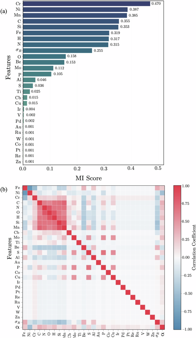
a MI scores of features for predicting α. This feature selection method indicates that Au, Co, Ir, Pd, Pt, Re, Ru, V, W, and Zn exhibit minimal relevance in the prediction of the target variable α. b Correlation Matrix. The relationships among features and target variable α are illustrated. The dataset shows a high level of multicollinearity among the chemical constituents. However, adding Au, Co, Ir, Pd, Pt, Re, Ru, V, W, and Zn correlates poorly with other variables, including α.

Full size image

For clarity, multicollinearity is often a concern in regression analyses, as variations of one predictor variable are interconnected with changes in other predictor variables. Particularly, multicollinearity makes it difficult to isolate and evaluate individual effects of explanatory variables on the target variable⁶³. This characteristic in the data underpins our selection of the XGBoost algorithm, as its regularisation and penalisation mechanisms mitigate multicollinearity effects. Nonetheless, optimal hyperparameter tuning is required to materialise the XGBoost’s advantages^64,65. The following section details the model optimisation process using nested cross-validation (CV) and Bayesian hyper-parameter optimisation (BHO), as well as the overall performance of the XGBoost regression model.

Evaluation of Model Performance

In this study, the framework provided by the Python libraries Optuna⁶⁶ and Ray⁶⁷ facilitated the implementation and monitoring of the nested CV protocol. An integral part of this process was employing the Box-Cox transformed values of α. This strategy not only normalises, but also ensures uniformity across different magnitudes of α. Thus, our predictions and error metrics are hereafter reported regarding the Box-Cox transformation.

Figure 4 summarises the performance evaluation of the XGBoost regression model during both, nested CV with BHO and the final training process. Figure 4a illustrates the BHO performance during the nested CV process, which evaluated 3000 hyperparameter sets. Here, high values of root-me represent pruned trials that the BHO method deemed unpromising. The optimal XGBoost configuration achieved a minimum root mean square error (RMSE) of 1.418 ± 0.12. Table 2 summarises the hyperparameter intervals for the XGBoost model and the optimised values obtained through nested CV with BHO.

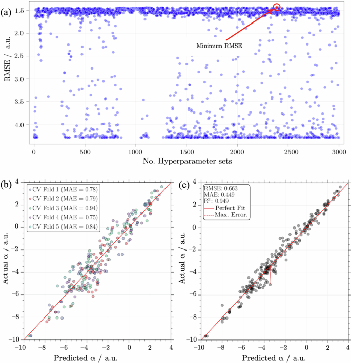
a Performance visualisation of nested CV coupled with BHO after evaluating 3000 hyperparameter sets. Here, the red point highlights the optimal XGBoost hyperparameter set, achieving a minimum RMSE of 1.418 ± 0.12. b XGBoost model performance across validation subsets during k-fold CV, with a MAE range from 0.75 to 0.94. c Overall performance of the XGBoost regression model, demonstrating the close fit between actual and predicted values of α values. Key metrics highlight the model’s predictive proficiency, with a high R² value of 0.949 and a low MAE value of 0.449, while an RMSE value of 0.663 indicates larger prediction deviations. The maximum error predicted was 1.408. All results and metrics are based on the Box-Cox transformed values of α.

Full size image

Figure 4b and c present the final phase results of the XGBoost model’s training and validation. Figure 4b compares the predicted and actual α values across CV folds (i.e., validation subsets). In this figure, the proximity of the points to the diagonal line indicates, in principle, that the model effectively avoids overfitting and can generalise well to unseen data⁶⁸. In terms of the mean absolute error (MAE), the XGBoost model’s predictions of α differ from actual observations in a range from 0.75 to 0.94.

Figure 4c further illustrates the XGBoost model’s performance, showing a good fit between the predicted and actual α values using the entire dataset. The maximum error made by the XGBoost regression model was 1.408, which is within the RMSE range observed during the nested CV process. The model’s prediction error was quantified using key metrics such as RMSE and MAE, which yielded values of 0.663 and 0.449, respectively. The low MAE demonstrates that, on average, the predictions made by our XGBoost regression model align closely with the actual αvalues. Apart from that, the coefficient of determination (R²) was 0.949, indicating the proportion of the variance in the target variable α that is predictable from input variables. In other words, the XGBoost regression model accounts for approximately 95% of the variability in the entire dataset.

Feature contribution analysis

Having an XGBoost regression model with adequate precision to predict α, we interpret the individual contributions of each input feature to the model’s output through permutation importance (PI) and SHAP. Figure 5 compares the results of these ML interpretation methods. In this case, PI provides a global overview of the feature importance in the XGBoost regression model. Comparatively, SHAP allows for a more granular understanding of feature effects at the level of individual predictions.

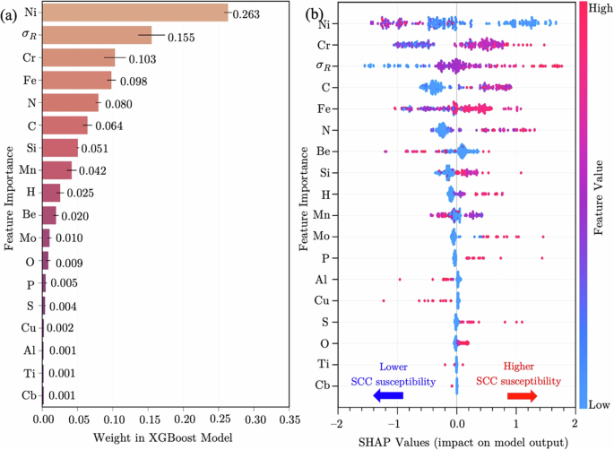
a Global impact of attributes based on PI scores. The error bars represent the standard deviation of PI scores. Significant additions of Ni, Fe, Cr, and ({sigma }_{R}) collectively provide a weight to the model’s output from 0.573 to 0.661. b Local contributions via SHAP values. Here, data points are spread horizontally, reflecting the feature effect on the model’s predictions. A rightward shift suggests higher α values and increased SCC susceptibility, while a leftward shift implies lower α values and reduced SCC vulnerability. The SHAP values are expressed in the Box-Cox transformed scale of α. The colour gradient going from blue (low) to red (high) indicates the influence of the feature magnitude.

Full size image

Figure 5a depicts the PI scores calculated using the Python package ELI5⁶⁹. The features are ranked in descending order of importance, allowing for the identification of key attributes that significantly impact the model’s performance. The PI approach centres on the premise that perturbing the values of a critical feature leads to a significant decrease in model accuracy. Thus, the PI scores indicate that Ni, with a weight of 0.263 ± 0.005, stands out as the most influential predictor in the XGBoost regression model. It is followed by ({sigma }_{R}), as well as Cr and Fe, with a weighted impact of 0.155 ± 0.019, 0.103 ± 0.15, and 0.098 ± 0.006, respectively. These results suggest that the XGBoost model’s predictions of α depend primarily on the concentrations of major alloying elements, coupled with the applied tensile loading. However, their combined influence results in a global impact ranging from 0.5733 to 0.661, meaning that the model’s outputs are considerably sensitive to minor additions, as their collective effect can vary from 0.311 to 0.349.

Figure 5b depicts the SHAP summary plot obtained via the TreeSHAP explainer implemented in the Python package SHAP⁷⁰. The features in Fig. 5b are arranged in descending order of importance based on the mean absolute value of their Shapley values across all samples. Each point represents a sample in the dataset, and its position on the horizontal axis indicates the feature’s impact on the XGBoost model’s predictions. Positive (rightward) shifts in SHAP values indicate an increase in the prediction of α values, suggesting a higher susceptibility to SCC. Conversely, negative (leftward) shifts indicate a decrease in the prediction of α values, implying reduced vulnerability to SCC. The colour gradient shows the feature’s magnitude, ranging from red for high values to blue for low values. For clarity, the specific ranges of feature values were previously reported in Table 1.

At an individual level, the SHAP values reveal feature contributions that align closely with the global results from PI. As shown in Fig. 5b, Ni remains the most influential factor in the XGBoost model’s predictions. Here, high Ni concentrations result in leftward shifts of SHAP values, indicating a decrease in the values of α, and thus enhanced resistance to SCC in boiling MgCl₂. Furthermore, Cr was identified as the second most important feature. Its position can be attributed, in principle, to its influence on improving localised corrosion resistance in chloride-rich environments⁷¹. This aligns with the established understanding that localised corrosion events often precede SCC¹¹. Interestingly, Fig. 5b reveals that high Cr concentrations (approaching a maximum 40 wt%) seem to render more vulnerable alloys to SCC in boiling MgCl₂, as indicated by the positive shift in the associated SHAP values. However, the distribution of negative SHAP values for Cr appears more heterogeneous than that of Ni, implying that its effect on α depends on the interaction with other alloying elements.

As seen in Fig. 5b, the significant impact of stress conditions is evident in the positive shift of SHAP values with the highest ({sigma }_{R}) (i.e., ({sigma }_{R}ge 1)). This observation indicates that plastically stressed samples experience a substantial increase in the predicted values of α, leading to accelerated SCC failures. Apart from this, samples containing additions of Be, Al, and Cu frequently resulted in a leftward shift in SHAP values, pointing out to an increase in SCC resistance. In contrast, the highest concentrations of other minor alloying elements (i.e., C, N, Si, H, Mo, Mn, and O) and impurities (i.e., P and S) consistently yielded positive SHAP values, suggesting a detrimental effect on SCC resistance.

Table 3 summarises the feature effects from the SHAP analysis on the XGBoost regression model (see Fig. 5b). Here, the mean absolute SHAP values and contributions to α are outlined for each feature, indicating their impact of on SCC resistance in boiling MgCl₂, as shown by the direction of SHAP values.

The specific contribution of Ni was further examined through the behaviour of SHAP values, as illustrated in Fig. 6. Interestingly, Ni content was found to modulate the impact of other input variables. This is observed in Fig. 6a, where a distinct shift in mean absolute SHAP values occurs when Ni content reaches 14.5 wt%. At this point, the mean SHAP score for Ni markedly decreases from 0.98 to 0.44, which is accompanied by a significant drop in the average impact of some minor additions, particularly C, H, Si, Mn, Mo, P, and S. While such alloying additions can be detrimental to SCC resistance, their diminished SHAP values beyond 14.5 wt% Ni suggest that their effects are relatively mitigated when Ni is present in higher amounts. In contrast, the mean absolute SHAP values for Fe, Cr, and ({sigma }_{R}) remain relatively stable across varying Ni levels, indicating a persistent influence (whether positive or negative) on predicting α and, therefore, on SCC resistance.

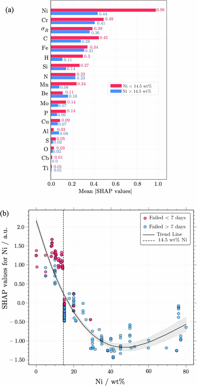
a Shifting feature impact with increasing Ni. The mean absolute SHAP values for Ni and minor alloying elements (mainly C, H, Si, Mn, Mo, P, S) change markedly at 14.5 wt% Ni, signalling a reduction in their impact on SCC susceptibility. b SHAP values as a function of Ni content illustrate the non-linear relationship between Ni concentration and SCC resistance. A maximum SCC resistance is observed around 40 wt% Ni, whereas SCC susceptibility increases when Ni content exceeds 45 wt%. The SHAP values represent the fluctuations of the Box-Cos transformed values of α. Data points are colour-coded to differentiate samples that failed within(red) and beyond (blue) seven days in boiling MgCl₂, as reported by Copson³⁴ and Staehle et al.³⁵.

Full size image

Figure 6b further elucidates the influence of Ni content on SCC resistance, as reflected through SHAP value behaviour. Here, a downward trend in SHAP values is observed as Ni content surpasses 14.5 wt%, indicating increasingly negative contributions to α, and thus a corresponding reduction in SCC susceptibility. In fact, most specimens with over 14.5 wt% Ni exhibited SCC resistance exceeding seven days in boiling MgCl₂, surpassing the median failure rate observed in the experiments of Copson³⁴ and Staehle et al.³⁵ In Fig. 6b, SHAP values reach a local minimum around 40 wt% Ni, indicating optimal SCC resistance at this concentration. However, as Ni content rises above 45 wt%, a notable increase in SHAP values is observed, signalling a decrease in SCC resistance. This trend aligns with experimental observations from Copson³⁴ and Staehle et al.³⁵, wherein samples containing 20−45 wt% Ni demonstrated superior durability in boiling MgCl₂ compared to those with greater Ni content. More importantly, these results highlight the XGBoost model’s ability to predict increased SCC susceptibility at very high Ni concentrations.

Analysis of model output

To showcase the explanatory capabilities of the XGBoost regression model and SHAP feature attributions, we examined the SCC resistance of four specific CRAs. In this analysis, we predicted α values of SS and Ni-base alloys using the XGBoost regression model. Subsequently, the most important features contributing to the predictions of α were interrogated through SHAP local explanations. Table 4 provides the chemical compositions of the selected samples, their performance during SCC testings in boiling MgCl₂, and the predicted values of α. As previously noted, the energy rate α was Box-Cox transformed to ensure data uniformity, allowing its use as a standardised proxy for evaluating SCC susceptibility, with lower values indicating reduced propensity for cracking.

Figures 7 and 8 present SHAP waterfall plots, which decompose local feature effects for the selected alloys into positive and negative contributions to α. The features are ranked by their absolute impact on the predictions. These plots enable a comparative analysis of the 10 most important features for each selected specimen. Essentially, the SHAP waterfall plots depict the input feature effects as cumulative steps, starting from an average prediction (i.e., base value ({phi }_{0}) = – 2.703) and sequentially building up to the final value of α through the influence of each feature.

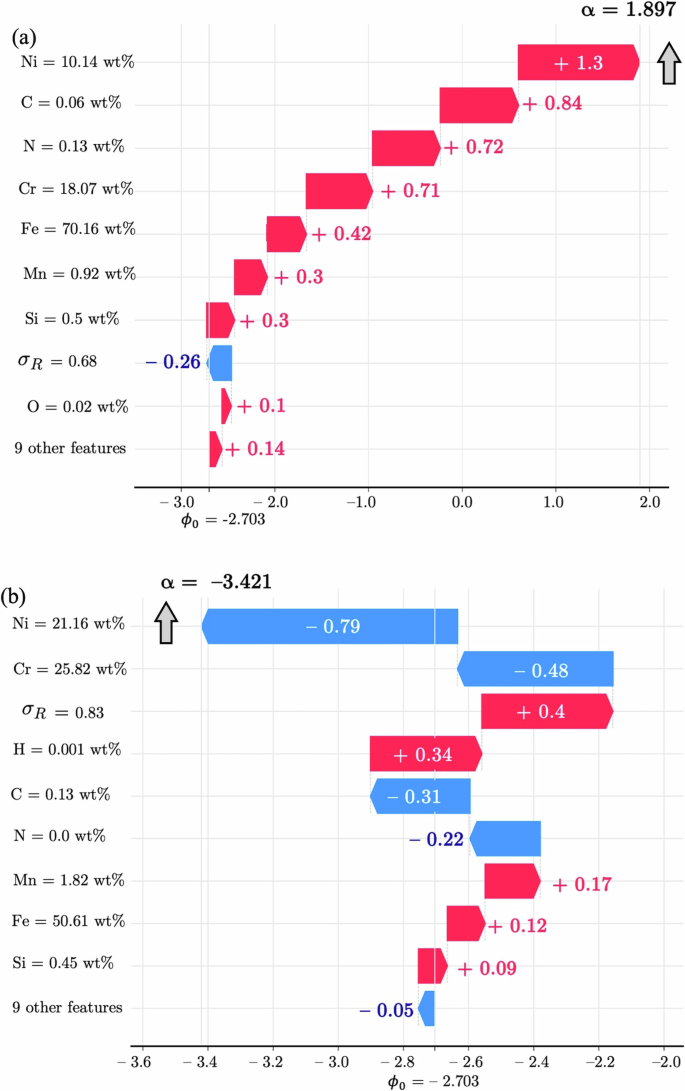
Comparative analysis of SCC susceptibility in SS alloys S30400 (a) and S31000 (b). Here, SHAP waterfall plots illustrate the contribution of each feature to the predicted energy absorption rate α. Each bar indicates the directional effect of a feature, with positive (red) contributions increasing α, and negative (blue) contributions decreasing α, starting from the base value ({phi }_{0}) = – 2.703. a The combined effect of alloying elements in S30400 results in a positiveα value of 1.897, indicating a relatively high susceptibility to SCC. b The high Ni and Cr content in S31000 contribute to a low value of -3.421, indicating enhanced SCC resistance.

Full size image

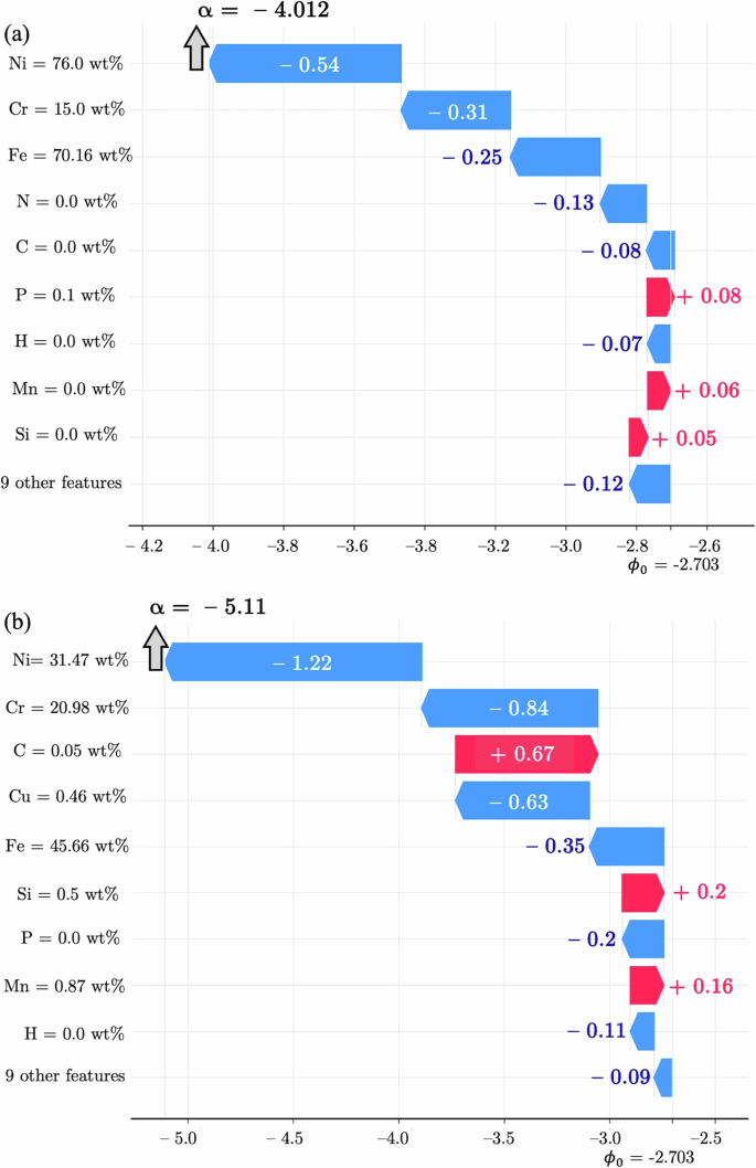
Comparative analysis of SCC susceptibility in Ni-base alloys N06600 (a) and N08810 (b). The bars represent a feature contribution to the predicted energy absorption rate α. Positive (red) contributions increase α, while negative (blue) contributions decrease α, starting from the base value ({phi }_{0}) = – 2.703. a In alloy N06600, Ni and Cr contribute the most to the α value of – 4.012, with other elements and ({sigma }_{R}) having minimal impact. b In N08810, the synergistic effect of Ni, Cr, and Cu results in a lower α value of – 5.11, enhancing its SCC resistance compared to N06600.

Full size image

Figure 7a and b compare two SS samples, alloys S30400 and S31000, respectively. Here, our XGBoost model predicted a considerably lower susceptibility to SCC for alloy S31000 (α = –3.421) compared to alloy S30400 (α = 1.897). This prediction aligns with the observed lifespans of these alloys in SCC testings with boiling MgCl₂, where specimen S30400 failed after 0.416 days, while specimen S31000 endured for 9.49 days. As illustrated in Fig. 7a, all interactions among chemical constituents in alloy S30400 synergistically contributed to a higher energy absorption rate α, even under a relatively low tensile stress (σ_R = 0.68). Comparatively, the bulk chemical composition of specimen S31000, particularly the high Ni and Cr levels, conferred significant SCC resistance. Figure 7b shows that despite being stressed slightly below its yield point (σ_R = 0.83), the combined effect of Ni and Cr justifies the S31000 sample’s resistance to SCC, accounting for over a third of the α value (i.e., –1.27).

Figure 8a and 8b compare two Ni-base samples, alloys N06600 and N08810, respectively. These specimens possess similar compositions and were tested under identical tensile stress conditions (σ_R = 0.9) in boiling MgCl₂. According to the XGBoost regression model, alloy N08810 has superior SCC resistance (α = –5.11) compared to alloy N06600 (α = – 4.012). These results are consistent with the experimental observations, where specimen N08810 endured 24.45 days in SCC testing, over twice as long as N06600. In Fig. 8b, SHAP analysis reveals that the synergistic effect of Ni, Cr, and Cu is the primary contributor to the enhanced SCC resistance of N08810. Specifically, the combined contribution of Ni, Cr, and Cu in N08810 accounted for over half of the total negative α value (i.e., –2.69). In stark contrast, specimen N06600 exhibited greater susceptibility to SCC despite its elevated Ni content, as shown in Fig. 8a.

Building upon the seminal investigations of Copson³⁴ and Staehle et al.³⁵, this study introduces a data-driven methodology to assess the susceptibility of Fe–Cr–Ni alloys to SCC. Unlike our previous publication³⁶, the current work moves beyond examining empirical observations (e.g., the beneficial effect of Ni), and leverages the XGBoost-SHAP analytical framework to quantify the impact of alloying elements and tensile stresses on SCC resistance. Central to our methodology was the use of the energy absorption rate α as a unifying metric, which enabled the XGBoost algorithm to infer how variations in alloy composition and loadings influence SCC failure rates in boiling MgCl₂.

Previous studies have explored using a single parameter to encapsulate the relationship between alloy composition, stress, and SCC susceptibility, although they have exhibited significant limitations. For instance, Parkins⁷² introduced the SCC index (SCI), which aimed to describe the effect of alloy composition and mechanical response on cracking propagation. The SCI was derived from linear regression analyses of time-to-failure data from SCC testings (i.e., SSRT and constant strain) and electrochemical potentials. However, this approach was limited in accuracy (i.e., R² ≈ 0.77) and failed to fully explain the influence of multiple alloying additions. Specifically, SCI models confirmed the positive impact of Cr and Ti on SCC resistance in a range of environments (i.e., nitrate, hydroxide, and carbonate-bicarbonate solutions), while the effects of other elements such as Mo, Cu, Ni, and Al remained unclear.

Similarly, Hines and Jones⁷³ investigated the effects of alloy composition on the SCC behaviour of austenitic Cr−Ni steels in boiling MgCl₂ using polynomial regression analysis. This study employed samples with varying Cr (8–26 wt%) and Ni (6–12 wt%) content, along with minor additions of C, Mo, Ti, Cu, Mn, and Si. The time-to-failure from constant-load tests served as the target variable in their regression models, while chemical compositions of specimens were used as predictors. The proposed polynomial model primarily elucidated the influence of minor additions, such as C and Mo. However, the individual contributions of Ni and Cr could not be discerned due to their mutual correlation, which is a common problem arising from multicollinearity between predictors.

The relationship between alloy composition and SCC resistance has also been associated with the stacking fault energy (SFE)⁷⁴. The SFE has been analysed as a predictor of SCC in various environments, including boiling MgCl₂⁷⁵. Here, materials exhibiting high SFE often demonstrated enhanced SCC resistance, whereas those with low SFE were more prone to cracking due to localised deformation mechanisms, chiefly transgranular SCC. In this context, linear regression models have been proposed to predict SFE values based on alloying additions in austenitic SS, thereby elucidating the impact of compositional variations on SCC susceptibility^76,77. These models successfully identified the positive influence of increased Ni content on SFE, correlating it with improved SCC resistance. However, the regression models were constrained to a few elements (i.e., Ni, Cr, Mn, Si) and did not fully capture the observed non-linearity between alloying additions and SFE.

Comparatively, the XGBoost-SHAP framework employed in this study effectively addresses the challenges of high-dimensional data and non-linear interactions inherent in multiple alloy systems. Notably, our ML regression model effectively isolated the effects of compositional variations and tensile stress, thus elucidating their bearing on SCC failure trends in boiling MgCl₂. For instance, the SHAP analysis of Ni’s influence on SCC resistance (see Fig. 6) revealed a critical threshold at 14.5 wt% Ni. Below this level, Fe-Cr-Ni specimens often failed within seven days, indicating a significant SCC vulnerability. This pattern appears to correlate with SCC susceptibility of SS alloys in hot chloride solutions, where intergranular and transgranular fractures initiated from localised attacks (i.e., pits) are commonly reported^78,79,80. Many of these SCC cases may, in turn, be influenced by minor additions (mainly C and Si), which can induce sensitisation, and thereby triggering localised changes in the passive film⁸¹.

Furthermore, our XGBoost regression model predicted increased SCC susceptibility when Ni content exceeds 45 wt%. This finding is consistent with other studies observing similar SCC failure patterns in high-Ni content alloys. For instance, Coriou⁸² reported that alloys with over 70 wt% Ni (i.e., N06600) often undergo SCC in pure and chlorinated water at elevated temperatures (i.e., ≥ 350 °C). However, alloys with 20–65 wt% Ni (e.g., N08800 and N06690) have demonstrated superior SCC resistance under these conditions^48,49. In boiling MgCl₂, alloys containing 30–34 wt% Ni have also exhibited comparable or slightly better resistance than those with 70 wt% Ni, predominantly failing through intergranular fracture^19,83.

The SHAP value analysis (see Fig. 5b) also highlighted that high Cr concentrations were detrimental to SCC resistance. This observation is consistent with our previous findings from Copson³⁴ and Staehle et al.³⁵, where samples exceeding 20 wt% Cr were susceptible to SCC in boiling MgCl₂, particularly when not balanced with sufficient Ni³⁶. Other investigations on SS alloys have shown similar results, where a Cr content up to 15 wt%, combined with around 10 wt% Ni, reduced SCC susceptibility^11,79. However, an increase in Cr content within the range of 18–25 wt% proved detrimental in boiling MgCl₂.

The XGBoost regression model also identified that stress conditions, particularly those inducing plastic deformation, can exacerbate SCC failure rates. However, it is important to note that certain alloy systems may not necessarily experience accelerated cracking under high-stress conditions, on account of the influence of specific minor additions. For example, Staehle et al.³⁵ observed that Fe-Cr-Ni alloys with Be additions did not fail after 30 days of exposure to boiling MgCl₂, even when subjected to constant tensile loads far exceeding their yield point (i.e., σ_R ≥ 1.5). This observation is supported by the SHAP analysis (see Fig. 5b), which showed a positive impact of Be additions on SCC resistance. The addition of Be is well-known to enhance the resistance of Ni-base alloys to SCC and CF at elevated temperatures, with optimal concentrations ranging from 1.8 to 2.75 wt%^25,84.

The XGBoost assesses other minor alloying elements in line with experimental observations in existing literature (see Table 3). For example, additions of Al and Cu have been proven to enhance SCC resistance. Specifically, adding Al up to 6 wt% promotes the formation of an aluminium oxide (Al₂O₃) film in both Fe- and Ni-base alloys, increasing their resistance to oxidation and sulfidation at high temperatures (i.e., over 600 °C)²⁵. In chloride-rich environments, such as boiling MgCl₂, Al additions above 0.1 wt% are reported to improve SCC resistance in a range of SS alloys⁸⁵, although Al was detrimental below 0.04 wt%⁵⁰. Similarly, Cu addition provides corrosion resistance in reducing acids and salts²⁵. Moreover, recent studies indicate that Cu enrichment (up to 5 wt%) decreases the severity of pitting corrosion in Ni–13Cr–10Fe alloys exposed to chloride environments⁸⁶. This has been attributed, in principle, to a reduction in the active dissolution rate within pits, and an increase in the local pit pH.

Conversely, the XGBoost regression model identified C, N, Si, Mn, Mo, P, and S as detrimental to SCC resistance in boiling MgCl_2. In this regard, numerous publications have extensively investigated their impact on cracking development in chloride-rich environments. For example, Loginow and Bates⁸⁷ reported the detrimental effects of increasing the N and C content (within the range of 0.001–0.1 wt%) in 18Cr–10Ni alloys when exposed to boiling MgCl₂⁸⁷. Similarly, N concentrations above 0.05 wt% have been associated with SCC of various 16–20Cr + 20Ni base alloys^20,21,50,51. The influence of Mn and Si appears to vary in boiling MgCl₂. Typically, the presence of Mn in SS does not effect SCC resistance unless its concentration is between 2–4 wt%^88,89. The addition of Si to Ni-base alloys is generally detrimental, although it has been observed to enhance the SCC resistance of SS, providing that the Si content remains below 2.0 wt%^25,43. In the case of Mo, it enhances the resistance of SS to pitting corrosion, although content exceeding 0.9 wt% has been shown to detrimentally affect the SCC resistance of 18Cr–10Ni alloys in boiling MgCl₂^17,90_. The synergy between P and S in both SS and Ni-base alloys is usually detrimental to cracking resistance^11,87. In this case, it has been experimentally observed that SS alloys can increase their resistance to SCC in boiling MgCl₂ when P content is below 0.003 wt%⁹¹.

Overall, the energy absorption rate α used for training our XGBoost model permitted a holistic assessment of factors contributing to SCC resistance. However, it is important to acknowledge that α is merely a theoretical construct designed to apply ML regression analysis. Therefore, the physical meaning and applicability of α require further validation. This could be achieved through experimental validation across diverse environmental conditions, or by developing a theoretical framework grounded in damage mechanics⁸⁸, aimed at linking α with underlying cracking mechanisms (e.g., dislocation dynamics or crack propagation). One potential path for theoretical work lies in energy-based descriptors such as fracture fatigue entropy (FFE)^89,92. It derives from irreversible thermodynamics principles and represents the accumulated entropy generated until fracture. Due to its material-specific nature and independence from testing conditions (i.e., frequency, stress amplitude, geometry, or environment), FFE is being employed in predicting the fatigue life of components under fluctuating damage conditions^93,94. Another limitation of the present study is the lack of microstructural information in the dataset (e.g., grain size and orientation, phase composition, precipitates), which is known to influence SCC occurrence. Additionally, the XGBoost model may be inadequate for evaluating alloys that exhibit singular effects in elastic properties, such as abrupt decreases in bulk or shear modulus due to the addition of specific alloying elements (e.g., Cr or Al). In this regard, no significant microstructural details or singularities in material properties were reported in the studies by Copson³⁴ and Staehle et al.³⁵

Despite the dataset’s limitations, the analytical framework combining the XGBoost algorithm and SHAP analysis yielded valuable insights into the influence of alloying elements on SCC resistance in boiling MgCl₂. By introducing the ratio between tensile toughness and time-to-failure, denoted as α, we were able to quantify SCC resistance and reveal the cooperative effects among alloy constituents. The synergy between the XGBoost algorithm and SHAP holds significant practical potential for materials engineering, allowing for exploring extensive compositional spaces with minimal experimental effort. Consequently, it can enable informed adjustments to concentration ratios in alloy systems, examining non-intuitive compositional combinations, and predictive assessments of material properties that enhance SCC resistance.

Dataset

We employ the dataset compiled by Rojas et al.³⁶, which contains the observations documented by Copson³⁴ and Staehle et al.³⁵ Table 1 provides a comprehensive overview of the 269 samples in this dataset, detailing their chemical composition, mechanical properties, tensile loading, and time-to-failure in SCC testing conducted in boiling MgCl₂.

Additionally, other features, such as stress ratio (({sigma }_{R})) and ({U}_{T}) were estimated for each sample in the data frame. Specifically, ({sigma }_{R}) refers to the ratio of applied load (({sigma }_{{app}})) to ({sigma }_{{YS}}) and enables the evaluation of the stress state of the samples, which can be elastically (({sigma }_{R}) < 1) or plastically (({sigma }_{R}) > 1) stressed. Hence, ({sigma }_{R}) is given by

Regarding ({U}_{T}), we approximate this property by calculating the area under the stress-strain curve defined by the Ramberg-Osgood equation of the form⁵⁷

wherein (sigma) is stress, (E) denotes Young’s modulus, (varepsilon) is the strain, and ({varepsilon }_{f}) represents the strain at failure. The constants, (H) and (n), represent the strength coefficient and the strain hardening exponent, respectively. To approximate (H) and (n), the elastic zone is assumed to be negligible, such that the yield point at a strain of 0.2% is within the plastic region of the stress-strain curve. Thereby, the values of (H) and (n) can be determined using the following expressions⁹⁵

Machine learning workflow

Figure 9 illustrates the three-stage workflow used in the current study. The initial stage relies on data preparation, comprising preprocessing and feature selection. These steps are critical for converting the dataset into a format suitable for training the XGBoost regression model. In this context, preprocessing involves configuring the input variables in relation to a designated target variable, which centres on ({U}_{T}). Here, the target variable was normalised using the Box-Cox transformation. This is a statistical technique that stabilises variance and makes data more normally distributed. It is particularly useful when dealing with non-linear, skewed, or heteroscedastic datam, which is is defined as⁹⁶

where (y) is the original data, and (lambda) is the power parameter. The optimal value of λ is chosen to maximise the normality of the transformed data, typically by using a maximum likelihood estimation method⁵⁸.

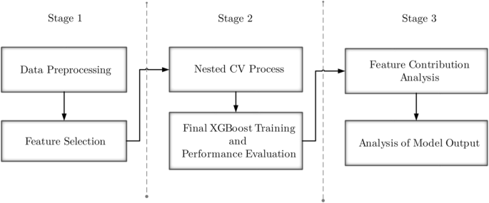
Three-stage workflow implemented for this study.

Full size image

Subsequently, feature selection is required to identify the most relevant predictors of the target variable. Further details on both the preprocessing and feature selection are outlined in the Results section. It is important to clarify that the XGBoost algorithm was primarily considered due to its capacity to handle substantial data dispersion, effectively model non-linear relationships, and demonstrate reduced sensitivity to outliers relative to linear or kernel-based models^64,97.

In the second stage, we employ a nested CV process with five resampling folds, which optimise the hyperparameters of the XGBoost regression model. This time-intensive procedure ensures that the model is finely tuned for maximum predictive accuracy. More importantly, nested CV allows for optimal utilisation of small datasets. It has been reported to be relatively free of bias and yields reliable results even with datasets containing fewer than 600 samples, as is the case with our dataset^98,99. It is noteworthy to specify that Bayesian optimisation is applied during the nested CV process, which efficiently explores the hyperparameter space, identifying the optimal combination that maximises the model’s performance, while minimising computational resources.

Thereafter, the overall model’s performance is rigorously examined through a final training and validation phase. Importantly, the nested CV and subsequent final evaluation employ three metrics to assess the performance of the XGBoost model: RMSE, MAE, and R², calculated as follows

where, ({y}^{(i)}) and ({hat{y}}^{(i)}) are the actual and predicted values, respectively, of the dependent variable for the i-th observation. The symbol (n) denotes the total number of observations, while (bar{y}) is the mean value of the dependent variable over all (n) observations.

The third stage focuses on the interpretative analysis of the XGBoost regression model, aiming to elucidate the contributions of each input feature to the model’s predictions. This is achieved through explainable AI methods, specifically PI and SHAP. In this feature contribution analysis, we quantitatively assess the synergies among alloying elements and their bearing on SCC resistance. Lastly, we further analyse the model’s ability to quantify SCC susceptibility of selected CRAs. Here, the XGBoost outputs are interrogated through SHAP feature attributions, offering a comprehensive assessment of how chemical constituents affect SCC resistance individually. The overview of the ML workflow provides the necessary context for the ensuing sections, which elaborate on the ML algorithms techniques employed in the present work.

Machine learning algorithms

Extreme gradient boosting

Developed by Chen and Guestrin³⁷, the XGBoost algorithm serves as a scalable and highly precise computational technique, which is applicable for classification and regression tasks in numerous domains¹⁰⁰. Fundamentally, XGBoost employs an ensemble learning strategy based on the gradient boosting (GB) framework, which was initially proposed by Friedman¹⁰¹. Therefore, the XGBoost algorithm generates a sequence of weak learners (i.e., classification or regression trees) designed to constitute the final predictive model⁹⁷.

In contrast to algorithms that construct regression trees in parallel (e.g., Random Forest¹⁰²), the sequential approach of XGBoost follows an additive training strategy⁹⁷. First, it trains a single tree to generate an initial prediction. Subsequently, the model is refined by introducing additional trees based on the residuals obtained⁶⁴. Thus, the output of the XGBoost model is the aggregation (either averaged or voted) of outputs from a series of trees, which may be expressed as

where K corresponds to the total number of trees, (k) represents the k-th tree, ({x}_{i}) is the feature vector corresponding to sample (i), ({hat{y}}_{i}) corresponds to the predicted score from this tree, while (F) is the space of regression trees.

Notably, the objective function in the XGBoost algorithm consists of two parts: 1) the loss function that measures the difference between the predicted values and the true values; and 2) the regularisation term, which controls the complexity of the model to prevent overfitting³⁷. Thereby, XGBoost is aimed at minimising the objective function (({obj})) expressed as

where (n) is the number of samples, ({y}_{i}) is the actual value of the i-th target; ({hat{y}}_{i}) is the predicted value of the i-th target. Hence, the (Lleft({y}_{i},{hat{y}}_{i}right)) is the training loss function that quantifies the discrepancies between predictions and data points, while(,varOmega left({f}_{k}right)) is the regularisation term that can be defined as

here, (T) is the number of leaves, and ({omega }_{j}) is the score of the j-th leaf. The coefficient (gamma) stands for the minimum loss reduction required to split a new leaf, while (lambda) is a regularisation coefficient.

During the boosting process, the predicted output is updated of the t-th iteration as follows

hence, the objective function takes the form

Particularly, XGBoost uses the second-order Taylor expansion of the loss function, which allows for faster optimisation and improved performance¹⁰³. The second-order Taylor expansion of the objective function can be written as

where ({g}_{i}) and ({h}_{i}) are the first and second-order derivatives of the loss function, respectively.

By combining the Taylor second-order expansion with the objective function and regularisation term, the approximated objective function becomes

where ({I}_{j}=left{i,|, qleft({x}_{i}right)=jright}) is the set of indices of data points assigned to the j-th leaf.

The XGBoost algorithm efficiently learns the tree structure and leaf weights by minimising the approximated objective function. The final equations for the optimal weight ({omega }_{j}^{* }) of leaf j, and the corresponding optimal value of the objective function ({{obj}}^{* }) are

Bayesian hyperparameter optimisation

Hyperparameter optimisation is critical for ML applications, as many algorithms rely on hyperparameters; these are settings that determine operational characteristics during training^104,105. For XGBoost and comparative ML algorithms, the hyperparameters play a critical role in shaping the model’s performance and generalisation capabilities¹⁰⁶. Nonetheless, identifying the most suitable hyperparameters is a challenging and labour-intensive task. It often necessitates navigating complex search spaces, which comprise numerous combinations of continuous, discrete, and conditional hyperparameters¹⁰⁷. To address this issue, BHO is extensively employed, as it builds a probabilistic surrogate model to predict the outcome of an objective function based on past evaluations¹⁰⁸. Thus, the surrogate model facilitates understanding the relationship between hyperparameters and model performance¹⁰⁹. In other words, BHO learns which regions in the parameter space are worth exploring and which are not by making full use of previous evaluation information¹¹⁰.

In the current study, we implement BHO using the tree-structured Parzen estimator (TPE) approach, obviating the need for predefined initial values or training sets^111,112. Initially, the TPE algorithm stochastically explores the hyperparameter space. The collected samples are then divided into two distinct categories. The first one includes the parameter samples that have been evaluated as the most effective based on a cost function, while the second consists of the remaining samples. Subsequently, TPE models the likelihood functions for these two categories: (l(x)) for the best-performing samples and (g(x)) for the rest¹¹³. The fundamental premise is to identify a parameter set that exhibits a higher probability of belonging to the first category. Thus, the expected improvement (({EI})) per iteration is calculated to guide the selection of new samples, which is given by¹¹⁴

Compared to traditional techniques, such as grid search and random search, BHO using TPE is advantageous due to its efficiency in exploring the parameter space, reducing computational complexity through skipping low-performing parameter samples^110,115. Moreover, BHO effectively finds optimal hyperparameters, especially for high-dimensional problems^115,116.

Nested K-fold cross-validation

Nested CV is a robust validation technique in supervised ML. This CV protocol performs outstandingly when hyperparameter tuning is integral to model building^117,118. Specifically, nested CV is based on the dual-layered partitioning of the dataset into multiple training and test subsets, thereby facilitating both hyperparameter tuning and model evaluation in a manner that minimises the risk of overfitting^119,120.

The nested CV protocol comprises two nested loops: 1) the inner loop for hyperparameter optimisation, and 2) the outer model-evaluation loop^119,121. The inner loop identifies the optimal hyperparameter values for the ML models. Subsequently, the model with the optimised hyperparameters is evaluated in the outer loop using a separate data partition, which was not involved in the hyperparameter tuning process. While computationally expensive, nested CV ensures that the evaluation metrics are not overly optimistic, providing a more realistic assessment of the model’s generalisability to unseen data¹²¹.

This study uses a nested CV process with five rounds of sequential hyperparameter tuning, combined with k-fold CV. As illustrated in Fig. 10, the dataset is randomly split into training and test subsets with a ratio of 80:20 (i.e., 80% of the data for training and 20% for testing). Each training subset within the outer loop is nested to a five-fold CV in the inner loop (with a validation partition equal to 10% of the outer training set), whereby potential hyperparameters for the XGBoost regression model are determined. The search for optimal hyperparameters is optimised via BHO throughout the five-fold inner CV. Subsequently, the XGBoost model performance is evaluated across all test folds in the outer loop. Upon the conclusion of the five rounds, the hyperparameter set achieving the highest accuracy is then selected.

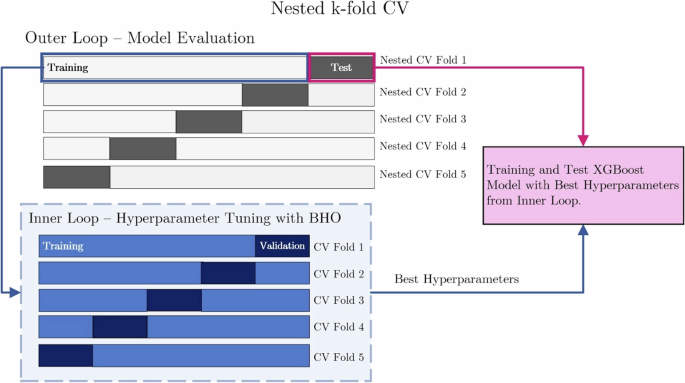
This method adjusts the XGBoost model’s hyperparameters using BHO, evaluates the model across all test folds, and selects the best hyperparameters after five rounds. Here, data is cycled through outer and inner loops to optimise the XGBoost model’s settings, improving its prediction accuracy. In the outer loop, data is partitioned into training and test subsets at a ratio of 80:20. Subsequently, within the inner loop, the outer training subset is further partitioned into training and validation sets with a ratio of 90:10.

Full size image

Permutation importance

In supervised ML studies, the PI method quantifies the impact of individual variables on the target outcome¹²². In this respect, Breiman¹⁰² and Fisher et al.¹²³ proposed a specific approach for PI analysis that divides the dataset into training and test subsets. Subsequently, a single model is trained using the training data. The test data for each input feature is then randomly permuted, and the model’s predictions are evaluated. If the performance decreases considerably, it indicates that the feature in question is critical for the model performance¹²⁴. Our work employs PI analysis to assess the specific weights associated with each input feature in the XGBoost model.

Shapley additive explanations

Shapley additive explanations employ a game-theoretic framework to elucidate the outcomes of an arbitrary ML model¹²⁵. Essentially, the SHAP approach is based on the Shapley value theory, a construct from game theory that fairly distributes the gain of a cooperative game among its players¹²⁶. In the context of ML, the features of a given data instance act as players in a coalition, and Shapley values tell us how to fairly distribute the payout (i.e., the prediction) among the features¹²⁷. In the context of SHAP, the model prediction is expressed as:

Here, (f({rm{x}})) represents the original model output, while (gleft({{rm{z}}}^{{prime} }right)) is the SHAP explanation model. The term ({phi }_{0}) is a base value when all inputs are missing, while ({phi }_{i}) corresponds to the SHAP value for the i-th feature, which quantifies the feature contribution to the difference between the actual prediction and base value. The term ({z}_{i}^{{prime} }in left{mathrm{0,1}right}) represents a binary variable, indicating the presence (1) or absence (0) of the i-th feature. Thus, SHAP decomposes the prediction into a linear combination of binary variables. M is the total number of features. Herein, we employ the SHAP method implemented for tree-based ensemble models, typically referred to as TreeSHAP¹²⁸.