Maximal steady-state entanglement in autonomous quantum thermal machines

Quantum thermal machines are open systems of interacting quanta that harvest spontaneous interactions with thermal reservoirs to perform a designated task. These machines have been proposed as quantum mechanical counterparts to the classical thermal machines of the industrial age, for instance, for work extraction, heating, cooling and keeping time^1,2,3,4,5. In recent years, they have also been implemented in experiments^6,7,8,9,10. However, quantum thermal machines can go further, and perform tasks that themselves are inherently quantum mechanical. The paradigmatic example is the generation of entanglement. It is well-known that entanglement can be generated via dissipation, and the topic has received much interest^{11,12,13,14,15,16}. When operating out-of-equilibrium, it is achieved by external driving of the system^17,18,19 or engineering of the quantum reservoirs^20,21,22.

This progress spurred the question of identifying the minimal resources to generate steady-state entanglement in dissipative out-of-equilibrium systems, i.e. with a time-independent Hamiltonian, no external work sources and no quantum bath engineering. The challenge is to rely only on spontaneous interactions with an uncontrolled environment while the system is not in equilibrium. Interestingly, an affirmative answer has been given. Two interacting qubits that are individually coupled to reservoirs of different temperature can end up in an entangled steady-state²³, due to a heat current through the system²⁴. Unfortunately, however, the generated entanglement is weak and unable to defy several notions of classicality²⁵. Going beyond the two-qubit systems, maximal entanglement is possible by using networks of several qubits^26,27. However, in aiming for a minimal machine that produces maximal entanglement, several works have considered supplementing the two-qubit system with some additional, non-autonomous, resources to amplify the two-qubit entanglement^{22,25,28,29,30,31}. Amplification of the entanglement has been possible also in the fully autonomous setting³², in particular by leveraging a voltage bias instead of a temperature bias³³. Nevertheless, none of these approaches have been able to deterministically generate maximal, or even nearly maximal, steady-state entanglement.

In this work, we identify the minimal thermal machine for generating any pure entangled state between the degrees of freedom of two physically separated qubits, using only time-independent, i.e. autonomous, resources. The machine exploits a chemical potential bias between two fermionic reservoirs at equilibrium, and involves three qubits subject to Coulomb repulsion and pairwise flip-flop interaction. Our machine, illustrated in Fig. 1a, thus uses the third qubit as a mediator for entanglement generation. Furthermore, we show that the machine performs well beyond the ideal regime of operation; reasonable Coulomb forces and potential biases, small detunings, and coupling strength variations all lead to nearly-maximal steady-state entanglement. Motivated by this, we investigate the conceptually deeper question of whether autonomous machines based only on two-body Hamiltonians are able to generate maximal entanglement between any number of qubits. We answer this in the positive by identifying a generalisation of our machine, which features 2n − 1 qubits, and prove that it can render n of these qubits in a W-type steady-state.

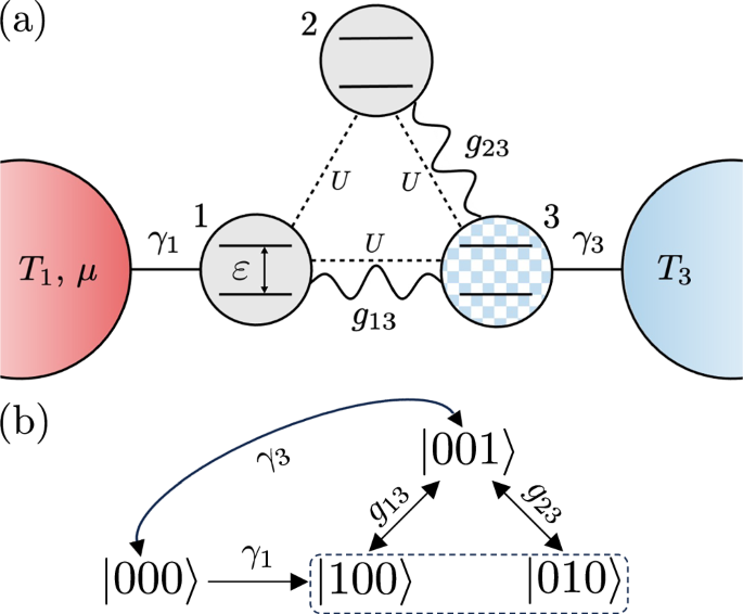
a The three-qubit autonomous thermal machine. The chemical potential of the left reservoir is the key resource for entanglement generation. The steady-state for the ideal regime of operation, has the solid gray qubits in the state (leftvert {Psi }^{-}rightrangle) while the shaded-blue qubit in the state (leftvert 0rightrangle). b A representative flow chart showing the relevant states of the three qubits. The states (leftvert 100rightrangle), (leftvert 010rightrangle) and (leftvert 001rightrangle) effectively form a lambda system⁴⁹. The dashed box indicates the entangled subspace corresponding to the steady-state.

Full size image

Model

We consider a setup of three interacting qubits, as shown in Fig. 1a. The excited state of each qubit corresponds to the energy gap ε. Qubit pairs 1-3 and 2-3 interact via flip-flop interactions with coupling strengths g₁₃ and g₂₃ respectively. Every qubit pair also interacts electrostatically via a Coulomb repulsion of magnitude U. The Hamiltonian of the three qubits is therefore given by (ℏ = k_B = 1),

where ({sigma }_{+}^{(j)},({sigma }_{-}^{(j)})) is the raising (lowering operator) for qubit j. Such a model can be realized in quantum dot systems³⁴ with spin-polarized electrons. For example, in Refs. ^35,36 such a triangular system was studied in a two-dimensional electron gas. The authors managed to bring all excitation energies into resonance³⁶ and suitable values of Coulomb interactions and tunnel coupling could be achieved³⁵. Alternatives could be based on pilar structures³⁷ or graphene bilayers³⁸, where such triple dots have been realized. A further interesting approach could apply ultracold fermionic atoms³⁹. Similar to the transport experiments^35,36, we take qubits 1 and 3 to be coupled to equilibrated reservoirs of non-interacting fermions, with bare coupling strengths γ₁ and γ₃. Throughout this article, we restrict ourselves to the regime of operation in which γ_j ≪ max{T_j, ∣ε ± g_ij − μ_j∣}, where T_j and μ_j are the temperature and chemical potential respectively, of reservoir j. Then, the evolution of the system can accurately be modelled by a Lindblad master equation. Further imposing g_ij ≪ max{T_j, ∣ε − μ_j∣} ensures that the dissipation acts locally on the qubits^40,41. Therefore, the Lindblad equation takes the following form,

where the dissipators are ({mathcal{D}}[L]rho :=Lrho {L}^{dagger }-frac{1}{2}left({L}^{dagger }Lrho +rho {L}^{dagger }Lright)) and ({gamma }_{jpq}^{+}) and ({gamma }_{jpq}^{-}) are the rates corresponding to transitions induced by the Lindblad jump operators L_jpq and ({L}_{jpq}^{dagger }). These are respectively defined as, ({L}_{1pq}:=leftvert 1pqrightrangle leftlangle 1pqrightvert) and ({L}_{3pq}:=leftvert pq1rightrangle leftlangle pq1rightvert). The exact excitation and relaxation rates are determined by the statistics of the reservoirs. For our reservoirs, we have that ({gamma }_{jpq}^{+}={gamma }_{j}{n}_{F}left(varepsilon +{{mathcal{U}}}_{pq},{mu }_{j},{T}_{j}right)) and ({gamma }_{jpq}^{-}={gamma }_{j}left(1-{n}_{F}left(varepsilon +{{mathcal{U}}}_{pq},{mu }_{j},{T}_{j}right)right)), where ({n}_{F}left(varepsilon ,mu ,Tright)=1/({e}^{(varepsilon -mu )/T}+1)) is the Fermi-Dirac distribution. ({{mathcal{U}}}_{pq}:=U{delta }_{p+q,1}+2U{delta }_{p+q,2}) takes into account the Coulomb interaction. It ensures that the potential energy difference of U is added for each additional excitation created in the system; U for a second excitation and 2U for a third. We take μ₁ = μ and for simplicity, we set μ₃ = 0 (Small variations in μ₃ have no impact on the generated entanglement in the ideal parameter regime and have negligible impact on entanglement when perturbed away from the ideal parameter regime). Therefore, the system is driven by two reservoirs which are out-of-equilibrium with each other. In the case of equal temperatures of the reservoirs, the imbalance is determined solely by the chemical potential of the left reservoir.

Generation of arbitrary pure entangled states

We now show that there exists an ideal parameter regime in which the steady-state solution to Eq. (2), when reduced to qubits 1 and 2, can correspond to any pure entangled state (up to local unitaries). As in Ref. ³³, we consider the limit in which

The first limit ensures that whenever there is already an excitation in the system, the fermions in either reservoir cannot overcome the large Coulomb interaction to excite the system further. On the level of rates, this translates to ({gamma }_{jpq}^{+}=0) whenever p + q ≥ 1. This eliminates the possibility of double or triple excitation in the three-qubit steady state. The second limit ensures that when there is no excitation in the system, the population in reservoir 1 is filled, i.e., n_F(ε, μ, T₁) = 1. The last limit is important to ensure that no double or triple excitations are possible at any point in the evolution of the machine. The reservoirs are therefore, extremely out-of-equilibrium with each other, with the left reservoir (coupled with qubit 1) at an extremely high bias and the right reservoir (coupled with qubit 3) at a low or zero bias. The only pathway for an excitation to leave the system is through qubit 3 and the right reservoir. We therefore refer to this qubit as the sink qubit. In the limits (3), the only relevant transitions are induced by the jump operators L₁₀₀, L₃₀₀ and ({L}_{300}^{dagger }). Note that one does not need to engineer the couplings to surpress the transitions corresponding to the other jump operators. in the considered limit, they become irrelevant regardless of their coupling strength. A matrix form of the Liouvillian ({mathcal{L}}) in these limits can be found in the Supplementary Information. The steady-state of the machine is the unique eigenstate of ({mathcal{L}}) with eigenvalue zero. The situation can be intuitively understood using the flow chart shown in Fig. 1b. As double and triple excitations are prohibited, only four classical states ((leftvert 000rightrangle), (leftvert 100rightrangle), (leftvert 010rightrangle), (leftvert 001rightrangle)) are relevant in the evolution of the machine. Two of these states, (leftvert 000rightrangle) and (leftvert 001rightrangle) are directly coupled to reservoir transitions and play no role at long times. In principle, a complex phase can be added in this superposition by using a magnetic field, through the Peierls subsitution method⁴². The steady state is pure and a superposition of (leftvert 100rightrangle) and (leftvert 010rightrangle),

which is actually a 1-particle energy eigenstate of the Hamiltonian (1). This state can be written as (leftvert {Psi }_{{rm{ss}}}rightrangle =left(cos theta leftvert 10rightrangle -sin theta leftvert 01rightrangle right)otimes leftvert 0rightrangle), with (theta :=arctan left({g}_{13}/{g}_{23}right)). Clearly, we obtain a partially entangled pure state between qubits 1 and 2, while qubit 3 is pushed into its ground state. The coefficients of the superposed states depend solely on the couplings between the qubits. Setting g₁₃ = g₂₃, we obtain a maximally entangled state in the form of the singlet (leftvert {Psi }^{-}rightrangle =left(leftvert 10rightrangle -leftvert 01rightrangle right)/sqrt{2}). Importantly, these results are independent of any temperatures of the reservoirs and the coupling rates between the latters and the qubits (within the ideal limit (3) and the validity of the master equation).

While Lindbladian evolution typically decoheres an initially pure state into a mixed state, it is generally possible to obtain a pure steady-state provided that certain conditions are satisfied. Firstly, the state (leftvert {Psi }_{{rm{ss}}}rightrangle) is invariant under the action of the jump operators L₁₀₀, L₃₀₀ and ({L}_{300}^{dagger }) which are relevant for the evolution. In other words, (leftvert {Psi }_{{rm{ss}}}rightrangle) is unaffected by the dissipators in Eq. (2) that remain after applying the limits (3). Secondly, this state is an eigenstate of the effective non-Hermitian Hamiltonian ({H}^{{prime} }=H-ileft({gamma }_{100}^{+}{L}_{100}^{dagger }{L}_{100}+{gamma }_{300}^{+}{L}_{300}^{dagger }{L}_{300}+{gamma }_{300}^{-}{L}_{300}{L}_{300}^{dagger }right)/2). These properties here ensure that (leftvert {Psi }_{{rm{ss}}}rightrangle) is the unique steady state of ({mathcal{L}}) under the considered limits^43,44. Using such reasoning, it can be shown that no two-qubit machine (autonomous or not) in the regime of validity of the local master equation can deterministically generate a pure entangled steady state, implying that our machine is minimal.

Minimality of the three-qubit setup

We now argue that a two-qubit machine cannot produce a Bell state as the unique steady state of local Lindbladian evolution considered in past works (e.g. in Refs. ^{22,23,24,25,33,41}). We assume a flip-flop interaction between the qubits, and that each qubit is individually coupled to a thermal reservoir. The Hamiltonian of the qubits is given by

where ({sigma }_{pm }^{(i)}) are the raisng and lowering operators of qubit i. There are a total of eight Lindblad operators corresponding to possible transitions that the reservoirs can induce,

We assume that the rates γ_j corresponding to these transitions can in general be distinct and can also be zero. The Lindblad equation then takes the form,

If there exists a steady state, it must satisfy ({mathcal{L}}{rho }_{{rm{ss}}}=0). Moreover, in the case of a pure steady state, (leftvert {psi }_{{rm{ss}}}rightrangle), we must have that all the dissipators annihilate this state, i.e., ({mathcal{D}}[{L}_{j}]leftvert {psi }_{{rm{ss}}}rightrangle leftlangle {psi }_{{rm{ss}}}rightvert=0)⁴⁴. To satisfy ({mathcal{L}}leftvert {psi }_{{rm{ss}}}rightrangle leftlangle {psi }_{{rm{ss}}}rightvert =0), we must also have that (-i[H,leftvert {psi }_{{rm{ss}}}rightrangle leftlangle {psi }_{{rm{ss}}}rightvert ]=0), i.e., (leftvert {psi }_{{rm{ss}}}rightrangle) must be an eigenstate of the Hamiltonian. Since the two Bell states (leftvert {Psi }^{pm }rightrangle =(leftvert 10rightrangle pm leftvert 01rightrangle )/sqrt{2}) are eigenstates of H, we try to see whether these states can be the steady state of Eq. (7). First, we note that these Bell states are annihilated by the dissipators ({mathcal{D}}[{L}_{1-4}]) but not by ({mathcal{D}}[{L}_{5-8}]). Therefore, from Eq. (7), we remove L₅₋₈ and are left with the following equation to check,

We note that while (tilde{{mathcal{L}}}) satisfies (tilde{{mathcal{L}}}leftvert {Psi }^{pm }rightrangle leftlangle {Psi }^{pm }rightvert {Psi }^{pm }=0), it does not have a unique zero eigenvalue and an initial-state-independent steady state in the usual sense. Specifically, in general, (tilde{{mathcal{L}}}) has two zero eigenvalues, which correspond to multiple fixed points of (tilde{{mathcal{L}}}). Moreover, due to the structure of the Lindblad operators, there can be residual oscillations even in the steady state (see, for example, Ref. ⁴⁵). This can be seen with a simple example. Suppose the system starts initially in the tensor product of the qubit ground states, (leftvert 00rightrangle). Then the system can gain an excitation on qubit 1 or 2 (through L₁ or L₂, respectively), but cannot gain a further excitation or lose one. Furthermore, through the flip-flop interaction Hamiltonian, the excitation continuously jumps from qubit 1 and 2, with a frequency that is determined by the coupling strength between the qubits. Therefore, a Bell state cannot be the unique steady state of the two-qubit machine and Eq. (7).

We note that the above discussion can be extended to any two-qubit Hamiltonian. To produce a steady Bell-state, the Hamiltonian must have this state as an eigenstate. The Hamiltonian (5) has (leftvert {Psi }^{pm }rightrangle) as eigenstates. We may instead consider another Hamiltonian that has (leftvert {{{Phi }}}^{pm }rightrangle =(leftvert 00rightrangle pm leftvert 11rightrangle )/sqrt{2}) as eigenstates. It can be checked that dissipators corresponding to the jump operators L₅₋₈ in Eq. (6) annihilate (leftvert {{{Phi }}}^{pm }rightrangle) into the null state, i.e., ({mathcal{D}}[{L}_{5-8}]leftvert {{{Phi }}}^{pm }rightrangle leftlangle {{{Phi }}}^{pm }rightvert =0). However, a Lindblad equation with just L₅₋₈ leads to similar problems as described above and the evolution is initial state dependent. For example, initial ground (leftvert 00rightrangle) and excited (leftvert 11rightrangle) states have no excitation or de-excitation channels, respectively. On the other hand, an initial state like (leftvert 10rightrangle) can evolve either to (leftvert 00rightrangle) or (leftvert 11rightrangle), with no further jump-channel and only the interaction Hamiltonian to control the dynamics. Therefore, no two-qubit Hamiltonian can possibly produce a perfect Bell state as the steady state of the two-qubit thermal machine.

Current at ideal operation

The average energy current, J, can be defined as the average rate of energy exchange between the system and reservoirs. Here, the energy current from reservoir j into the system takes the form⁴⁶,

In our convention, the heat flow from a reservoir to a qubit is positive, while the other way round is negative. Therefore, currents from the high bias and low bias reservoirs have opposite signs and the average current can be naturally defined as (J(t):=left({Q}_{1}(t)-{Q}_{3}(t)right)/2).

Since at long times, the third qubit is completely depopulated, no excitation can travel into the right reservoir. Moreover, due to the large chemical potential, no excitation can travel back into the left reservoir. As a result, there cannot be any current between the system and reservoirs in the steady state despite the reservoirs being heavily out-of-equilibrium with each other. Therefore, (leftvert {Psi }_{{rm{ss}}}rightrangle) is a dark or non-conducting steady-state of the machine, similar to the works^47,48.

In Fig. 2a, we plot the energy current as a function of time with the three qubits initially in the ground state (leftvert 000rightrangle). This is merely a relevant example since the steady-state (4) holds for any choice of initial state. As expected, we find that the initially non-zero energy current drops to zero. We note that a deviation from the ideal limits (3) drives the system to a mixed “bright” steady state exhibiting a non-zero energy current. However, this state can still be considerably entangled, as discussed below.

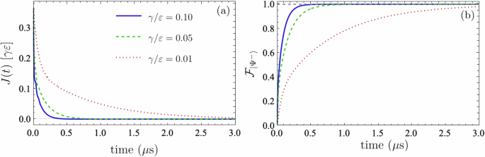
a Energy current and (b) fidelity with (leftvert {Psi }^{-}rightrangle otimes leftvert 0rightrangle) as a function of time, with the parameters ε = 1 GHz, T₁ = T₃ = T = ε, γ/ε = γ₁/ε = γ₃/ε, g₁₃/ε = g₂₃/ε = 0.05, U → ∞, μ → ∞, U/μ → ∞ and system-reservoir couplings as given in the legend. The qubits are initially in the ground state (leftvert 000rightrangle).

Full size image

We remark that in the absence of dissipation, (leftvert {Psi }_{{rm{ss}}}rightrangle) is a time-independent solution of the Schrödinger equation for the three levels (leftvert 100rightrangle), (leftvert 010rightrangle) and (leftvert 001rightrangle). Therefore, these states effectively form a lambda system with the couplings g₁₃ and g₂₃ playing the role of Rabi frequencies of a probe field. The three-qubit state is coherently trapped⁴⁹ between the states (leftvert 010rightrangle) and (leftvert 100rightrangle) with coefficients determined by the couplings.

Time-scale and entanglement generation away from ideal operation

Although the maximally entangled state can be obtained independently of the couplings and temperatures (as long as g₁₃ = g₂₃), the couplings to the reservoirs determine the time-scale at which the steady state is reached. Specifically, the larger the coupling, the shorter the time-scale. In Fig. 2b, we plot the fidelity of ρ(t) with the state (leftvert {Psi }^{-}rightrangle otimes leftvert 0rightrangle), with the system initially in the ground state (leftvert 000rightrangle). Choosing the natural frequency of the qubits as 1 GHz. 1 GHz is, for example, the relevant scale for state-of-the-art superconducting platforms⁵⁰. For semiconductor quantum dots, the scale can be one or two orders of magnitude larger, we find that the steady state can be reached within a few microseconds for all three considered coupling strengths. This is only a relevant example; the relaxation time scale is determined by the Liouvillian eigenvalue having the largest (smallest negative) real part. This is controlled specifically by the system-reservoir couplings. Therefore, this time-scale is the same for any initial state and of the order of magnitude of 1/γ.

In Fig. 3, we investigate the quality of the generated entanglement with respect to changes in the system’s parameters, i.e., away from the limits in Eq. (3). In such a situation, all possible classical states of the three-qubit system are involved in the dynamics, including at long-times. The solution must therefore take into account all possible transitions induced by the jump operators L_jpq and ({L}_{jpq}^{dagger }) in the general Lindblad equation (2). As a measure of entanglement, we use the concurrence, which for the state of qubits 1 and 2 can be written as (C(rho )=2,,{text{max}},{0,| c| -sqrt{{p}_{11}{p}_{00}}}), where c is the coherence corresponding to element (leftvert 01rightrangle leftlangle 01rightvert) and p₁₁(p₀₀) is the probability corresponding to the state (leftvert 11rightrangle leftlangle 11rightvert (leftvert 00rightrangle leftlangle 00rightvert)). We find that large entanglement can be created with reasonable Coulomb interaction and chemical potentials. As expected from the previous discussion, to generate a large amount of entanglement, we also find that U should be chosen to be sufficiently larger than μ. For instance, choosing U = 15T and μ = 8T (where T₁ = T₃ = T) yields a concurrence greater than 0.99, while μ = 15T with the same Coulomb interaction yields only 0.25. This is due to the presence of double excitations coming from the left reservoir when the Coulomb interaction is not large compared with the chemical potential. Overall, we note that the scheme requires the Coulomb interaction and chemical potential to be much larger than the qubit energies and the temperatures. In the Supplementary Information, we also consider variation in the coupling rates γ₁ and γ₃, as well as the influence of single-qubit dephasing.

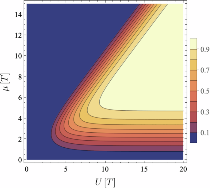
Near-maximal entanglement is obtained for a large range of parameters, such that μ/T and U/T are both sufficiently larger than 1.

Full size image

Our analytical results have been obtained using the Lindblad equation (2) with local coupling, which restricts to individual transitions between reservoirs and qubits. In order to assess the validity of this approach, we have shown numerical calculations with the second-order von Neumann approach^51,52 using the QMEQ package⁵³ in the Supplementary Information. This approach includes cotunneling events, partially lifting the blockade of current in the steady state. For larger system-reservoir coupling, we find only a minor reduction in the entanglement, as quantified by the concurrence (still above 98% for parameters from Fig. 3). In addition, we find that Lamb-shift terms lead to a slight change in the resonant condition between the qubit energies. Importantly, both effects vanish with decreasing system-reservoir coupling. More details can be found in the Supplementary Information.

Multipartite entanglement generation

A natural question is whether autonomous resources and two-body interactions can go even further and produce maximally entangled states of many qubits. A naive approach is to add a fourth qubit in the system in Fig. 1 and coupling it to the sink qubit, but this does not yield multipartite entanglement or even a unique steady state. The reason for this is similar to the explanation in Sec. IIC. For successful operation, i.e., to produce a unique pure entangled steady state, the scheme requires coupling to a filled reservoir, as well as an exit way for excitations through the sink qubit. In the absence of such exit ways, there will be oscillations due to inter-qubit couplings even at long times. Therefore, the additional qubit to be entangled requires its own, additional, sink qubit. That is, to generate maximal genuine multipartite entanglement between three qubits, we use two auxiliary qubits serving as sinks. This is illustrated in Fig. 4. This idea can be directly extended to an arbitrary number of qubits; for every additional qubit to be entangled, we couple it to the qubit already connected to the high-bias reservoir, and then we add a corresponding sink qubit. This can be seen as many ‘triangles’ of qubits, within each of which we have an electrostatic interaction between every pair and a flip-flop interaction between the sink qubit and the other two qubits (in complete analogy with the original machine in Fig. 1). In this way, we can deterministically generate an n-qubit W-type entangled state in a (2n − 1)-qubit autonomous thermal machine. Under the same limits as the two-qubit case, namely Eq. (3), we show in Supplementary Information that this scheme corresponds to a generalised coherent population trapping over n states (instead of just two), which renders the steady state of this scheme pure and entangled. Specifically, it is

where (leftvert {bar{0}}_{k}rightrangle :=leftvert 0rightrangle otimes leftvert 0rightrangle otimes cdot cdot cdot otimes leftvert 0rightrangle) is the ground state of k qubits and

(leftvert {Psi }_{,text{ss},}^{n}rightrangle) corresponds to a W-type partially entangled state for qubits 1 − n. The condition to obtain maximal entanglement is similar to the three-qubit machine. Here, if the inter-qubit couplings within each triangle are equal, i.e., g_1,n+j = g_1+j,n+j or α_j = 1, (leftvert {Psi }_{,text{ss},}^{n}rightrangle) corresponds exactly to the following W state of n qubits, while n − 1 qubits are pushed into their ground state,

(leftvert {W}_{n}rightrangle) denotes a W state in the space of n qubits and a ground state in the next n − 1 qubits. In this enumeration, the first system is the high-bias qubit and the ground state (leftvert {bar{0}}_{n-1}rightrangle) corresponds to all the sink qubits. For simplicity, in Fig. 4, we have chosen all temperatures and all qubit-reservoir couplings to be equal. However, this is not a necessary condition to produce a (leftvert {W}_{n}rightrangle) state. The couplings can be chosen almost arbitrarily (within the validity of the Lindblad equation) and the temperatures have to be chosen such that U ≫ μ ≫ T_j. Robustness to variations in system-reservoir couplings are further discussed in Supplementary Information.

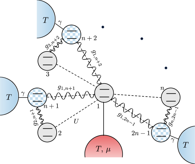
An n-qubit W state is now obtained between qubits 1,2,…,n (gray), while the sink qubits (n + 1),(n + 2),…,(2n − 1) (shaded, blue) are pushed to their ground state. The dashed lines represent Coulomb interaction with strength U, and the wiggly lines represent inter-qubit coupling between qubits i and j with strength g_i,j. For simplicity, we have chosen the temperatures and system-reservoir couplings to be equal. For n = 2, the machine reduces to the one in Fig. 1a, producing (leftvert {Psi }^{-}rightrangle otimes leftvert 0rightrangle) when the inter-qubit couplings are equal. For each additional qubit to be entangled, one extra sink qubit and one extra “triangle” are necessary in the setup.

Full size image

A considerable number of earlier works on autonomous entanglement generation focussed on creating two-qubit entanglement using a setup of two qubits. The amount of entanglement in these works was always noisy and far from maximal. In this work, we have shown that this is limited due to the structure of the Lindblad equation – it is impossible to generate a perfect Bell state using a a two-qubit autonomous thermal machine. Importantly, we have introduced a minimal three-qubit architecture that generates a steady Bell state for ideal operation. The scheme is robust; even away from ideal operation, it can generate near-maximal entanglement. Furthermore, we have demonstrated that our results can be extended to producing genuinely multipartite entanglement in the form of W states of an arbitrary number of qubits. It is an interesting theoretical question whether our ideas can be extended to produce arbitrary pure entanglement, in particular, the Greenberger-Horne-Zeilinger states⁵⁴ and whether it is possible to obtain high-dimensional entanglement⁵⁵ in a similar setting.

While maximal entanglement generation is possible with non-autonomous resources such as driving¹⁹ and athermality³¹, our work provides a fully autonomous pathway to generating maximal entanglement. In other words, our work demonstrates that pure dissipation into thermal environments is sufficient to generate the strongest forms of quantum correlations. This reveals the striking fundamental power of autonomous evolution.

Finally, beyond their fundamental significance, we believe that recent developments in quantum technologies make our predictions experimentally feasible. While there are many platforms that may be suitable, electronic quantum dots are a natural candidate. Here, the right coupling regimes (within the validity of our master equation) can be already engineered in triple-dot setups^35,36. Crucially, Coulomb repulsion is naturally present and bias voltage (and therefore the chemical potential) can freely be controlled, making the operation of the setup possible close to the ideal limit.