Microscopic parametrizations for gate set tomography under coloured noise
Introduction
Unlocking the full potential of quantum information processors (QIPs) is a multifaceted challenge that requires key advances along various directions, both technological and fundamental1. Among these, the development of efficient techniques for the characterization of undesired interactions – or noise – in QIPs, is of particular relevance, for it allows to develop improved strategies to counter its undesired effects. This is the case of some schemes2 of quantum error mitigation3,4,5,6, or some strategies7,8 for quantum error correction9,10,11 that may allow to find shortcuts towards the fault-tolerant era. In pursuit of this goal, the community working in quantum characterization, verification, and validation (QCVV) has devised a wide variety of methodologies12,13,14. Some of these approaches seek to provide a unified metric to estimate device performance without explicitly detailing the form of the errors, as exemplified by randomized benchmarking15,16,17,18,19. Others strive towards a precise prediction of the actual faulty operations in the noisy QIPs, belonging to the family of quantum tomography techniques20,21.
The simplest protocol that falls in this category is quantum state tomography (QST)22,23,24,25,26,27, which aims to estimate an unknown quantum state described by a unit-trace positive-semidefinite linear operator in a Hilbert space ({mathcal{H}}) of dimension (d=dim ({mathcal{H}})), namely (rho in {mathsf{D}}({mathcal{H}})subset {mathsf{Pos}}({mathcal{H}})). For discrete-variable systems, QST requires implementing measurements drawn from an informationally complete (IC) set of positive operator-valued measure (POVM) elements ({{M}_{mu }:,mu in {mathbb{M}}}), where ({M}_{mu }in {mathsf{Pos}}({mathcal{H}})) and ({sum }_{mu }{M}_{mu }={{mathbb{1}}}_{2})28 (see Fig. 1a). These allow for an univocal estimate (hat{rho }) of the state ρ from the observed probabilities ({p}_{mu }={rm{Tr}}{{M}_{mu }rho }), where we will use hats to differentiate the statistical estimates from the actual objects (see Section I of the supplementary material). In quantum process tomography (QPT)29,30,31,32,33, the focus lies on the estimation of the quantum channel (rho mapsto {mathcal{E}}(rho )), a completely-positive and trace-preserving linear operator ({mathcal{E}}in {mathsf{C}}({mathcal{H}})subset {mathsf{L}}({mathcal{H}})) that describes a physically-admissible operation on a quantum system transforming input to output states1,28,34,35. In addition to the above IC measurements, an IC set of initial states ({{rho }_{s}:,sin {mathbb{S}},,| {mathbb{S}}| ={d}^{2}}) is also required to perform QPT. See Fig. 1b for a schematic representation of QPT. Similarly to QST, one can find an univocal estimate of the channel (hat{{mathcal{E}}}) from the measured probabilities ({p}_{mu s}={rm{Tr}}{{M}_{mu }{mathcal{E}}({rho }_{s})}).
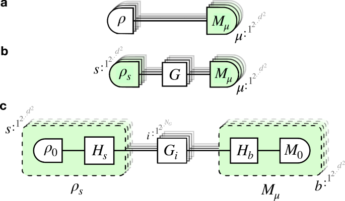
a State tomography. An informationally complete set of d2 predetermined POVM elements {Mμ} needs to be specified. b For process tomography, in addition to the POVM elements, an IC set of d2 initial states {ρs} must also be specified. c Gate set tomography. The QPT scheme must be executed for each of the NG gates at the set. These gates, or combinations thereof (denoted by Hs and Hb), act on a single experimentally-accessible initial state ρ0 and POVM M0 to obtain the aforementioned IC sets.
In practice, however, any real experiment will only provide an approximation to above POVM probabilities given a finite number of measurement shots. We consider from now on that each POVM is described by a measurement basis b and a possible outcome mb, such that (mu =(b,{m}_{b})in {mathbb{M}}={{mathbb{M}}}_{b}times {{mathbb{M}}}_{{m}_{b}}). This is the case of the Pauli measurements in N-qubit systems with d = 2N, where the POVM elements can be defined in terms of the orthonormal Pauli basis ({E}_{alpha }in {{{{mathbb{1}}}_{2},{sigma }_{x},{sigma }_{y},{sigma }_{z}}}^{{bigotimes }^{N}}/sqrt{d}). Each Pauli measurement outcome is binary mb = ± 1, and the specific number of outcomes ({N}_{b,{m}_{b},s}) that result from Nb,s measurement shots per initial state and measurement basis lead to a binomial distribution with relative frequencies ({f}_{mu ,s}={N}_{b,{m}_{b},s}/{N}_{b,s}). In the asymptotic limit Nb,s ≫ 1, this tends to a normal distribution ({f}_{mu s} sim N(bar{mu },{bar{sigma }}^{2})) centred around the aforementioned probabilities (bar{mu }={p}_{mu ,s}) with standard deviation (bar{sigma }=sqrt{{p}_{mu ,s}(1-{p}_{mu ,s})/{N}_{b,s}}). Hence, there are intrinsic finite-sample errors that describe the deviations from the probability distributions pμs, which are typically referred to in the literature as quantum projection or shot noise36.
In analogy to QST, one can obtain a linear relation between measured relative frequencies and the quantum channel acting as a super-operator37. For instance, using the so-called Pauli Transfer Matrix (PTM) representation (see Supplementary Section I of the supplementary material), the linear equations can be straightforwardly inverted. However, this linear inversion can lead to non-physical estimates of the channel (hat{{mathcal{E}}},notin ,{mathsf{C}}({mathcal{H}})) when finite-sample errors are significant. To avoid these problems, maximum likelihood estimation is typically preferred38, as the numerical optimization of a cost function can be supplemented with constraints to ensure that all estimated channels are indeed physically acceptable31,32. One of the advantages of this strategy is that the constrained optimization problem is convex and, thus, a unique estimate (hat{{mathcal{E}}}) is guaranteed.
Gate set tomography (GST) (Fig. 1c) was introduced to overcome a fundamental shortcoming of QPT39,40,41,42,43. QPT, although used in several QIP platforms44,45,46,47,48,49,50,51,52, suffers from a self-consistency issue: it assumes that the IC set of initial states and measurements are error free. In reality, however, these states are usually obtained by acting with a set of gates {Gi} on a single fiducial state ρ0, which reduces to (leftvert 0rightrangle leftlangle 0rightvert) in the ideal N = 1 case. Likewise, the measurements are obtained by acting with these gates on a single binary projective measurement ({M}_{z,+}={M}_{0},,{M}_{z,-}={mathbb{1}}-{M}_{0}), which reduce to (leftvert 0rightrangle leftlangle 0rightvert ,leftvert 1rightrangle leftlangle 1rightvert) in the ideal N = 1 case. Clearly, {Gi} are implemented similarly to the noisy gate (hat{{mathcal{E}}}) that we aim at characterizing, and will thus contribute to a non-zero state preparation and measurement (SPAM) error. In the case of single-qubit gates, this error will be of the same of order as the one that afflicts the gate we want to estimate. It is thus not justified to assume that the SPAM is ideal and error free. GST addresses this self-consistency issue by targeting the full set of noisy elements, including the gates used to attain IC as well as the fiducial operators in a full “gate set”
As emphasised in ref. 39, QPT is not device-independent in its entirety, as it requires a prior independent calibration of the measurement basis and initial states. GST eliminates this requirement and provides a complete self-consistent characterization that treats the whole QIP device as a black box. However, to attain this full generality, it requires at least NGST = NG × 4N(4N −1) + 23N −1 parameters for an N-qubit system, where ({N}_{G}=| {mathbb{G}}|) is the number of gates in the set (1). Estimating these parameters thus requires an exponentially-large number of imperfect fiducial state preparation, followed by a combination of gates from the gate set, and a final fiducial imperfect measurement. In addition to this exponential scaling, one has to account for the number of samples required to achieve a target precision ϵ. In the case where resources are evenly allocated among a fixed set of base circuits, as conceived in the early GST proposals, this number increases as Nb,s ∝ 1/ϵ2. Altogether, the resource scaling limits the applicability of a fully-general GST to systems with small qubit numbers. The development of long-sequence GST is a significant advancement in this regard39, which estimates the gate set parameters using data from specific circuits that are built from combining elements of the gate set. This protocol linearly amplifies gate parameters as the circuit depth p increases, allowing for a Heisenberg-like scaling of the precision estimates. In particular, in the asymptotic limit, the error falls with the inverse of the circuit depth and not with its square root, as would occur if one only used the resources to increase the number of repeated measurements in circuits that only involve a single gate in addition to the SPAM ones.
The full generality of GST is convenient to validate and verify the functioning of a certain QIP device, regardless of having any specific microscopic knowledge, making it useful for external users. On the other hand, it can also help developers to calibrate their devices and guide hardware progress in the current noisy intermediate scale quantum (NISQ) era53. From that perspective, one can benefit from a microscopic modelling of these devices to partially alleviate the stringent resource requirements of GST. In this work, instead of using a device-agnostic approach, we advocate for a microscopically-motivated parametrization of the gate set (1), having a specific setup in mind: gates mainly limited by coloured phase noise. This is motivated by recent experiments with trapped-ion devices, from which one can extract that phase and frequency fluctuations dominate noisy single-qubit gates54,55,56,57. Since these two contributions affect the qubit dynamics in a similar manner, one typically refers to their combination as phase noise. Additionally, because amplitude noise fluctuations can also be included in our model, we expand our analysis to account for the so-called universal stochastic noise when adding this source of imperfections, which is subdominant in the case of trapped ions. As discussed in ref. 57, the effect of frequency and phase stochastic fluctuations of current trapped-ion QIPs can be accurately described with the filter-function formalism58,59,60,61,62,63,64,65. We use this formalism to demonstrate that the imperfections of the gate set can be related to various filtered integrals of the noise spectral density, reducing considerably the number of parameters that is required in GST. In particular, for the gate set under study in this work, the total number of parameters for fully-general approach amounts to NGST = 67. This contrasts with that required to characterize the gate set under the coloured phase noise, where NGST = 11 is required for a Markovian estimation or NGST = 16 for a non-Markovian one. We do also show that it is straightforward to account for amplitude noise fluctuations as well, at the cost of just two additional parameters in order to completely characterize the gate set.
The preceding discussion motivates the main idea behind the present study: using a physically-motivated version of GST to alleviate the computational cost required for its execution, while being sufficiently general to capture the primary sources of imperfections in target devices, such as trapped-ion processors. Additionally, the work addresses key technical challenges associated with the numerical implementation of the protocol. Notably, it eliminates gauge redundancy and significantly simplifies the processes of circuit selection and fiducial pair reduction required in fully general GST. These advances represent the core contributions of this study. Finally, we refer to the GitHub repository ColouredGST66 as a guide for the numerical implementation of the results.
This manuscript is organized as follows: subsections “Filtered-noise parametrization of the gate set”, “Microscopic parameters and gauge redundancy”, “Long-sequence maximum-likelihood estimation” and “Selection of parametrized base circuits” in the Results section present the theoretical description of our parametrized GST. We delve into some peculiarities derived from this microscopically-motivated approach, such as the simplification of the circuit selection process and the absence of the so-called gauge redundancy, which is a characteristic of fully-general approach to GST39,40,41,42. Subsections “Numerical benchmarks with stochastic noise”, “Comparison with fully-general GST” and “Inclusion of amplitude noise fluctuations” constitute a numerical validation of our parametrized GST. By considering specific numerical simulations of the coloured phase noise, we can compare the GST estimates (hat{{mathcal{G}}}) to the exact microscopic operations (bar{{mathcal{G}}}) that stem from the stochastic averages over the phase fluctuations. In this way, we can analyse the accuracy of our estimation and discuss its performance for different noise regimes, including the effect of time correlations and non Markovian evolution as well as the amplitude noise extension of the model. Moreover, we compare the results of our parametrized GST approach with those obtained from fully general GST applied to the same numerically-simulated data. We close this manuscript with the Discussion section, highlighting conclusions and mentioning future research lines motivated by this work.
Results
The goal of this section is to give a comprehensive account of our customized GST, comparing the parameterization for the phase-noise model on single-qubit gates to the standard protocol of long-sequence GST. For a review of important aspects of GST, see Supplementary Subsection I of the supplementary material, where we focus on the concepts used throughout this work, which are discussed in more depth in the review by Nielsen et al.39 for fully-general GST. As outlined in the introduction, the main advantage of employing a microscopically-motivated model lies in the reduction of the parameters required for a complete self-consistent characterization.
Although approached from a different angle, using a simplified model to efficiently learn the noise of a device is successfully exemplified by van den Berg et al.2, where one restricts the estimation to a Lindblad-Pauli channel67,68. In fact, for a Lindbladian evolution, one can estimate the generators of the channel rather than the channel itself, which allows to reconstruct the full dynamical quantum map44,69,70,71,72,73,74,75,76, and obtain advantages from compressed sensing when the microscopic noise generators have a clear structure with leading components77. In some situations, however, time correlations in the noise and non-Markovian effects forbid this approach. Moreover, the Pauli-type channel may also be a crude approximation to the actual native gate set. As shown in this work, even in this situations, one can still benefit from a detailed microscopic modelling of the non-Lindblad and non-Pauli channel through a reduced parametrization of GST. This reduction not only leads to significant savings in computational resources, but also results in a proportional decrease in the number of experiments required. Moreover, as we describe now in detail, our approach circumvents certain challenges encountered in a fully-general GST.
Filtered-noise parametrization of the gate set
As discussed in the introduction and in subsection I of the supplementary material, GST considers a noisy gate set (1), which can be described using the process matrix representation for the quantum channel associated to each gate
Here, (left{{E}_{alpha }:alpha in {1,cdots ,,{d}^{2}}right}) can be any basis of the space of linear operators ({mathsf{L}}({mathcal{H}})), such as the aforementioned Pauli basis1. The above set of {χ(i)} matrices must be semidefinite positive and fulfill a so-called trace constraint (chi in {mathsf{Pos}}({{mathbb{C}}}^{{d}^{2}}),{sum }_{alpha ,beta }{chi }_{alpha ,beta }{E}_{beta }^{dagger }{E}_{alpha }={{mathbb{1}}}_{{d}^{2}}). In full generality, each of them must be parametrized via d2(d2 −1) real parameters. The fiducial operators ({rho }_{0},{M}_{0}in {mathcal{G}}) require NSPAM = d3 −1 real parameters, leading to a total of NGST = NG × d2(d2 −1) + d3 −1 parameters to be estimated in GST.
Rather than treating the QIP as a black box and aiming at GST with full generality, we advocate for a specific parametrization that employs a physically-motivated microscopic modelling of the gates. To define a gate set, let us start by considering the case of perfect unitary gates
where θi(ϕi) is the pulse area (phase). In this work, we will slightly abuse the notation by using the same symbol Gi for the unitary gate, its Pauli transfer matrix representation, and the gate label. IC can be achieved by using a single θ = π pulse with ϕ = 0 that maps (leftvert 0rightrangle leftlangle 0rightvert mapsto leftvert 1rightrangle leftlangle 1rightvert), and a pair of θ = π/2 pulses with ϕ = 0 and ϕ = 3π/2, which map (leftvert 0rightrangle leftlangle 0rightvert mapsto leftvert +rightrangle leftlangle +rightvert) and (leftvert 0rightrangle leftlangle 0rightvert mapsto leftvert +{rm{i}}rightrangle leftlangle +{rm{i}}rightvert), respectively, where (leftvert pm wrightrangle =(leftvert 0rightrangle pm wleftvert 1rightrangle )/sqrt{2}). These π/2 pulses also suffice to rotate the measurement basis from b = z to b = y, x, achieving the required IC. In the context of long-sequence GST, it will be convenient to enlarge this gate set to NG = 5 by also including the inverse of the π/2-pulses, as this does not require additional parameters when considering the microscopic noisy gates, and can lead to a higher sensitivity of the circuits to the parameters that long-sequence GST aims at estimating. We thus define our gate set
where we have introduced the following angles
In an experiment, the gates Gi will deviate from the ideal unitaries (3). One common source of noise that appears in several platforms and limits the gate fidelities is that of phase noise, which can be modelled by a particular stochastic process and characetrised by its experimentally-measurable power spectral density S(ω). As detailed in the Methods section, this experimental information could enable us to adapt our GST to a specific QIP. In the same section, we further argue that a inferring the noisy gates from an estimation of this quantity using qubit noisy spectroscopy lacks self-consistency, reinforcing our paranetrized GST as the appropriate method. As we also detail in the Methods section, a dressed-state master equation for the description of the noisy gates, one can find a parametrization of the process matrices (2) that can be specified by only four real parameters ({chi }^{(i)}left({Gamma }_{1}({t}_{i}),{Gamma }_{2}({t}_{i}),{Delta }_{1}({t}_{i}),{Delta }_{2}({t}_{i})right)). In turn, these parameters incorporate information of the noise and the single-qubit driving leading to the gate, which are encapsulated in filtered integrals of the power spectral density (PSD)
Here, the filter functions ({F}_{{Gamma }_{n}}(omega ,{Omega }_{i},{t}_{i}),{F}_{{Delta }_{n}}(omega ,{Omega }_{i},{t}_{i})) are explicitly given in Eqs. (29–33), where we note that ti(Ωi) stands for the pulse duration (Rabi frequency) of each gate. It is interesting to observe that the noisy gates ({G}_{i}^{{rm{id}}}({theta }_{i},{phi }_{i})mapsto {G}_{i}({theta }_{i},{phi }_{i})) in Eq. (4) with shared pulse duration ti and Rabi frequency Ωi, such that the pulse area θi = Ωi ti is the same, are actually described by the same filtered noise parameters under our noise modelling and, furthermore, these parameters do not depend on the driving phases ϕi in Eq. (5). The only change for different gates is that the microscopic parameters enter in different places of the corresponding process matrices, as detailed in Section I of the supplementary material. Hence, no additional effort will be necessary to characterize G3(π/2, 3π/2), G4(π/2, π/2), G5(π/2, π) via GST under the assumption that G1(π, 0), G2(π/2, 0) can be estimated efficiently. In fact, including these operations in the gate set can lead to an improved parameter sensitivity in long-sequence GST.
Let us note that the standard approach of GST emphasises the requirement of a Markovian evolution during the noisy gates, and a failure in the gate set reconstruction can sometimes be associated to a model violation due to the breakdown of the the Markovianity assumption39. On the other hand, when considering the full PSD of the phase noise (6), we are indeed incorporating finite time correlations (21), and thus deviating from a purely Markovian prediction base on a Lindbladian approach. Hence, the discussion about Markovianity and GST is slightly more succinct. As detailed in57, one can rigorously connect the values of the filtered noise parameters {Γn(ti), Δn(ti)} to a non-Markovianity measure78,79,80,81,82 that is based on the lack of a completely-positive division of the resulting quantum dynamical map83,84. If we include Γ2(ti), Δ2(ti) in the noisy gate set parametrization, and the GST estimates that these parameters are indeed non-zero, the reconstructed gate set corresponds strictly to a non-Markovian quantum evolution. Hence, GST can indeed estimate non-Markovian gates, albeit assuming that there are no time correlations in between the SPAM operations and the different gates in the GST sequence, i.e. we assume that the noisy parametrization of each gate is independent of the previous history of gates applied within a given sequence. Considering that the coloured noise will have a characteristic correlation time τc, we are thus assuming that ti/τc can be sufficiently large so that non-Markovian effects take place during each gate, but the time in between consecutive gates Δti,j ≫ τc, such that one can neglect correlations between different gates.
In principle, one could exploit the formalism of the noise filtered integrals to extend the modelling of fluctuations also in between gates, accounting for non-Markovianity in the full gate sequence. However, the resource cost of GST would increase considerably, as each circuit of the long-sequence GST would then depend on the specific gate history, and thus require even more parameters to be estimated. Some proposals of non-Markovian tomography have already been made employing tensor networks85,86, always at the expense of an even greater computational cost. We leave a detailed study of these questions for future work.
In most of the discussion below, we will show that the leading-order effect of the noisy gate set can be characterized by restricting to a non-zero Γ1(ti) and Δ1(ti), whereas Γ2(t) = Δ2(t) = 0. It is worth noting that, under this Markovian assumption, the total number of parameters – and minimal number of experiments – required to completely characterize this gate set decreases from NGST = 67 when working with the fully general description of the channels to NGST = 11 with our parametrized approach. In the last part of subsection “Numerical benchmarks with stochastic noise”, we present a generalization of our parametrized GST to allow for non-zero {Γ2(ti), Δ2(ti)}, where we quantify how certain noise regimes require GST to account for these non-Markovian effects in order to achieve higher accuracies.
As a summary of our previous discussion, we now emphasize the core results of our phase-noise parameterization. First, we highlight the significant reduction in terms of experimental cost enabled by the estimation of the filtered parameters (6) rather than the elements of the quantum channels without modelling. Second, we point out the ability to capture certain non-Markovian effects at a moderate cost. As already described, there are situations in which the gate set can be accurately estimated by a subset of the mentioned filtered parameters. Nonetheless, including the whole set of parameters permits us to describe situations in which Markovian contributions cannot be neglected. In the next subsections, we will also show that certain technicalities of the computational implementation of GST are simplified with our parameterization.
Microscopic parameters and gauge redundancy
Once the gate set and its parametrization have been described, we can discuss the different estimation strategies for GST. As reviewed in Supplementary Section I of the supplementary materials, the first schemes of GST41 considered a linear-inversion scheme that only requires measuring the probabilities of simple circuits composed of the SPAM operations and the action of the individual gates ({G}_{i}in {mathcal{G}}) (see Fig. 1c). This approach leads to a certain redundancy in the estimated gate set (hat{{mathcal{G}}}) found by linear GST. As discussed in that section, it is easy to see in the super-operator formalism in which states and measurements are vectorized (vert {hat{rho }}_{0}rangle rangle ,langle langle {hat{M}}_{0}vert), and quantum channels have a matrix representation ({hat{G}}_{i}), that one can apply a similarity transformation T to obtain a new gate set ({{hat{mathcal{G}}}}{^{prime}}) that is equally valid when one transforms simultaneously the estimated noisy gates and the fiducial state and measurement operators
This redundancy in linear GST is referred to as gauge freedom, and arises due to the absence of a privileged reference frame, which is the price to pay when transitioning from QPT to GST. Moreover, it is actually not exclusive to GST but also appears in other characterization techniques such as randomised benchmarking87.
When using a parametrized gate model, this redundancy may be partially or even completely eliminated, as the microscopic modelling can actually define a privileged reference frame. This is precisely the situation for our Markovian parametrization, which only depends on the filtered-noise parameters that do not change under any similarity transformation. Under this transformation, the matrix structure of our parametrization of the noisy gates must be preserved, as it describes the whole family of imperfect gates subject to the coloured phase noise, albeit with a different set of parameters ({{Gamma }_{1}({t}_{i}),{Delta }_{1}({t}_{1})}mapsto {{Gamma }_{1}^{{prime} }({t}_{i}),{Delta }_{1}^{{prime} }({t}_{1})}). Considering that under a similarity transformation ({hat{G}}_{i}^{{prime} }={T}^{-1}{hat{G}}_{i}T), both ({hat{G}}_{i}) and ({hat{G}}_{i}^{{prime} }) must possess the same spectrum, one can readily see that our parametrization does not allow for gauge redundancy. By calculating the eigenvalues of the corresponding noisy gates, we find that (sigma ({G}_{i}({Gamma }_{1},{Delta }_{1})),ne ,sigma ({G}_{i}({Gamma }_{1}^{{prime} },{Delta }_{1}^{{prime} }))) for any physically-admissible (({Gamma }_{1}^{{prime} },{Delta }_{1}^{{prime} })), where σ(O) symbolizes the spectrum of the operator O. This indicates that there is only one pair of parameters consistent with the GST probabilities.
The absence of gauge redundancy renders unnecessary the need for gauge optimization techniques used in fully-general GST39. Usually, these techniques are required to compute distance metrics, which depend on the gauge choice, adding further complexity to the already demanding estimation process of GST. Typically, the gauge-fixed gate set is defined as the one that is closest in a certain notion distance to the ideal unitary gate set (3), while being compatible with the measured frequencies. Due to its simplicity, we will opt for trace distance (T(rho ,{rho }^{{prime} })=frac{1}{2}sqrt{{(rho -{rho }^{{prime} })}^{dagger }(rho -{rho }^{{prime} })}) to get a measure of ‘closeness’ between a reconstructed gate set element and a target one1. Note that the (in-)fidelity88 is not a wise choice in this context, as it is only well-behaved for normalized density matrices, and not every element in our gate set satisfies this condition. For our parametrization, the trace distance between two gates is
which will be useful to estimate the error in our parametrised GST, where we will compute an average trace distance for all elements in the gate set (trace distances for the fiducial elements are introduced at the end of the next subsection). We do not need to delve here into whether gauge fixing by minimizing the trace distance to the unitary gates is a fully-consistent technique or not, as one could imagine sufficiently-noisy instances in which, by minimizing the distance to the unitary gate set along a gauge orbit, one is actually moving further apart from the actual noisy channels that represent the imperfect gate set. This problem is entirely absent in our case, as there is no gauge redundancy left in our parametrization.
Long-sequence maximum-likelihood estimation
Let us now discuss the posterior GST developments that superseded linear GST41, showing that one can improve the accuracy and precision of linear GST estimates by allowing for sequences of gates forming more complex circuits. This leads to the concept of long-sequence GST (see Fig. 2) briefly discussed in the Methods. In this subsection, we begin by introducing these concepts and then focus our discussion on their application to the phase noise model. This leads to a simplification of the constraints imposed during optimization and a significant reduction in the complexity of identifying the experiments required for GST (see Subsec. “Selection of parametrized base circuits”). Together with the previously discussed absence of gauge redundancy, these represent the main technical advantages of our approach.
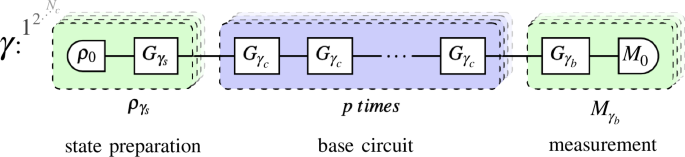
The conventional long-sequence GST scheme uses Nc different possible combinations of circuits, here labelled by γ, that contains the state preparation γs, base circuits γc, and measurement γb sublabels. When preparing IC sets of initial states ({rho }_{{gamma }_{s}}) and POVM elements ({M}_{{gamma }_{b}}), we rely on the action of single gates. For our parametrization, the base circuit germs germs ({G}_{{gamma }_{c}}) are also single gates, as these are a valid amplificationally complete set (see Sec “Selection of parametrized base circuits”). Each circuit results in d possible outcomes resulting from the binary Z-basis measurement for each qubit.
Let us introduce γs, γc, and γb as labels of the different state preparation, base circuit and measurement basis components of a particular circuit γ = (γs, γc, γb), respectively. The probability characterizing the measurement outcomes of each of the NC circuits in long-sequence GST can be expressed in terms of the corresponding product of parametrized process matrices
where ω = (α, β, τ, ζ, ϵ, δ) ∈ {1, ⋯ , d2} is a super-index that labels the components of the process matrices in the Pauli basis for each part of the GST circuit. We recall that these matrices are expressed as products of the parametrized χ(i) matrices of the individual noisy gates as shown in Supplementary Subsection II of the supplementary material, each of which has a non-linear dependence on the noise-filtered integrals (6)({chi }^{(i)}({{{Gamma }_{n}({t}_{i}),{Delta }_{n}({t}_{i})}}_{n = 1,2})). We group all of these parameters, together with those of the fiducial operations, in a single vector θ, which will allow us to formalise the GST as a particular problem of multi-parameter point estimation38.
To avoid non-physical estimations in GST, one defines a cost function that depends on the differences between these parametrized circuit probabilities and the corresponding measured relative frequencies fγ(mb), which is then minimised under specific constraints to restrict to physically-admissible gate sets. Following some of the ideas used in fully-general GST39, we integrate a negative log-likelihood cost function ({{mathcal{C}}}_{{rm{ML}}}({boldsymbol{theta }})) with a weighted least-squares cost function ({{mathcal{C}}}_{{rm{LS}}}({boldsymbol{theta }})) throughout the iterative process that minimizes
In our optimization routine, we choose circuits with a maximum depth that is logarithmically spaced, and run an optimization iteration for each of them, incorporating data from lower depths into the larger-depth subsequent steps. Additionally, the solution obtained from each iteration serves as the initial guess for the subsequent one, using the ideal unitary gate set as the initial guess for the first iteration. This workflow, originally developed for fully-general GST, prevents us primarily from getting stuck at an undesirable local minima of the cost function, but also from increasing the potential ‘branch ambiguity’ with depth. This problem occurs when any of the parameters under estimation is multi-valued, such that (theta to theta {rm{mod}},K). Then, the Heisenberg-like increase of accuracy stemming from considering deeper versions of the circuits also increases the multi-value ambiguity, so that one has (theta /pto theta /p,{rm{mod}},K/p). Lu ckily, the inclusion of the previously mentioned logarithmically spaced maximum depth circuits is sufficient to discern the ‘true’ branch. Regarding the cost function, we opt for ({{mathcal{C}}}_{{rm{LS}}}) during the optimization involving the initial low-depth stages, while ({{mathcal{C}}}_{{rm{ML}}}) is employed at later stages when a sufficiently accurate estimation has already been reached at previous iterations that can be used for the initial guess of the subsequent ones, as this can correct for the potential biased behaviour of ({{mathcal{C}}}_{{rm{LS}}}) for rare events39. We remark that the choice among the cost functions is rather heuristic, and may vary depending on the structure of the problem.
So far, the definition of the optimization in Eq. (10) is not complete, as we have not detailed yet the constraints. Working with the process matrix representation (2), we need to impose the already mentioned positive semi-definite and trace preservation constraints. These conditions manifest neatly with our approach, as our parametrized process matrices are always trace preserving, while the only condition required to ensure complete positivity in the Markovian regime reduces to Γ1(ti) ≥ 0. Additionally, we restrict ρ0 and M0 to be positive semi-definite, and set the trace of the fiducial state to be unity. Consequently, the minimization (10) must be constrained as
From this point onward, we adopt the orthonormal Pauli basis with N = 1 for single-qubit systems. With this basis, the native state and measurements can be expressed as ({rho }_{0}=frac{1}{sqrt{2}}left({E}_{0}+mathop{sum }nolimits_{alpha = 1}^{3}{r}_{alpha }{E}_{alpha }right)) and ({M}_{0}=frac{1}{sqrt{2}}left(mathop{sum }nolimits_{alpha = 0}^{3}{e}_{alpha }{E}_{alpha }right)) respectively, where rα, eα are real coefficients. Then, constraints on ρ0 and M0 can be further simplified to
In contrast to fully-general GST39, in which the CPTP conditions are not imposed when working with the Pauli transfer matrix representation of a quantum channel (see the Methods section), the former physical constraints are notably simpler and can be readily imposed during the optimization stage independently of the channel representation. Note that, in parallel with the expression in Eq. (8), these parametrizations for the fiducial elements lead to the simple trace distances ({T}_{{hat{rho }}_{0},{bar{rho }}_{0}}=sqrt{mathop{sum }nolimits_{alpha = 1}^{3}{({hat{r}}_{alpha }-{bar{r}}_{alpha })}^{2}}) and ({T}_{{hat{M}}_{0},{bar{M}}_{0}}=sqrt{mathop{sum }nolimits_{alpha = 1}^{3}{({hat{e}}_{alpha }-{bar{e}}_{alpha })}^{2}}).
Selection of parametrized base circuits
Having covered the main aspects of our parametrized approach to GST, we can now discuss how to select a set of base circuits that permit achieving an increased sensitivity in the estimation of the filtered noise parameters. In this subsection we interweave a discussion of general circuit selection with its simplified counterpart for single-qubit phase noise. The conclusion is clear: base circuits that form a minimal set and yield more accurate results than a general approach at the same circuit depth.
The efficacy of long-sequence GST hinges on the capability of amplifying each model parameter in θ by the repetition of base circuits p ≫ 1 times. This enables a reduction of the estimation uncertainty Δθp = Δθ/p, where Δθ denotes the uncertainty for a single repetition p = 1. This contrasts the reduction of the shot-noise uncertainty mentioned in the introduction, which scales with the number of shots used to infer the relative frequencies as (1/sqrt{{N}_{{rm{shots}}}}). This idea, first explored in ref. 41, has evolved into its current form described in ref. 39 for fully-general GST, including steps of so-called circuit/germ selection and fiducial pair reduction that we now consider for our parametrized GST.
In long-sequence GST, one has to carefully determine a set of germs – circuits composed of gates from the gate set – that suffice to amplify each gate-set parameter when repeated p times. These sets, coined amplificationally complete (AC), rarely result in a one-to-one correspondence between circuits and parameters, as there are many circuits with specific combinations of gates that end up amplifying common gate-set parameters. In addition, evaluating the outcome of every of these germ circuits for all SPAM operations on the fiducial pair of initial state and measurement ρ0, M0 increases the total number of circuits considerably. This can actually waste resources in terms of experimental shots for certain measurements that do not give more information about the parameters. In essence, there are redundant combinations of base and SPAM circuits that increase the number of experiments beyond a minimal GST design, and it is thus important to develop techniques for circuit selection (CS) and fiducial pair reduction (FPR) to reduce this redundancies39. In this way, the measurement resources can be optimally used for those AC circuits that provide more information gain.
Interestingly, we can actually avoid this two-step CS and FPR process by demonstrating that our parametrized gates already constitute an AC set, and there is no need to combine them in more complicated circuits. This enables us to effortlessly identify minimal GST designs that are optimal for single-qubit gates. Finally, as explained before, our restricted model does not suffer from gauge redundancy, obviating the need for additional gauge optimization techniques to establish a common reference frame to compute distance metrics.
In fully-general GST, one identifies an AC set of germs ({g}_{i}={G}_{{i}_{1}},{circ}, {G}_{{i}_{2}},{circ}, ldots ,{circ}, {G}_{{i}_{N}}) by finding non-vanishing quantities for
where τ(gi) stands for the Pauli transfer matrix for the germ gi. The general approach to calculate this amplification gradient uses Schur’s lemma to establish a relationship between the expression above and the derivative when p = 1, under the assumption that τ(gi) is approximately unitary39,89. This assumption remains valid for the high-fidelity QIPs until the number of repetitions of the germs is too large, and the accumulated error starts to dominate leading to a deviation from the unitary behaviour. This transition typically occurs at depths that are considerably larger than 1/ϵ, where ϵ is defined as the decoherence rate per gate. In combination with experimental limitations, this error accumulation prevents one from using arbitrarily long circuits in GST to enhance the estimation accuracy and precision.
Fortunately, due to the simplicity of our parametrized expressions for the noisy gates, we can evaluate the expression (13) analytically. Furthermore, considering single-gate germs with a Markovian parametrization of the phase noise, we find ({[{G}_{i}({Gamma }_{1}({t}_{i}),{Delta }_{1}({t}_{i}))]}^{p}={G}_{i}(p{Gamma }_{1}({t}_{i}),p{Delta }_{1}({t}_{i}))), which is indeed the amplification behaviour one looks for when executing long sequence GST. This behaviour is consistent with the fact that every parameter describing our model appears at least in one eigenvalue of the model gates. Coming back to Eq. (13), we note that each of the non-vanishing matrix elements in this limit, denoted here by the indices (j, k), satisfies
leading directly to two conclusions. Firstly, as anticipated by the linear amplification of parameters with p, the individual gates indeed serve already as valid germs for long-sequence GST. This becomes evident by evaluating Eq. (14) in the high-fidelity regime (pΓ1(ti) ≪ 1). Typically, short germs are prioritized to maximize precision when constrained by a maximum circuit depth, so this is significant. In addition, as we are not combining different gates to form germs, the sets of parameters that different germs amplify are disjoint. The resulting experiments are therefore identical to Rabi sequences (for π-pulses) or those commonly employed in multipulse Ramsey spectroscopy (for π/2-pulses)90,91,92, in contexts such as atomic clock characterization. Secondly, as we will discuss latter, we can use this limit to predict the region in which the error dominates, corresponding to p ≳ 1/Γ1(ti), where long-sequence GST will not lead to further improvements on the accuracy and precision of the estimation. It is significant to mention that individual gates are no longer sufficient to perform long sequence GST when the Markovian approximation is relaxed (Γ2(ti), Δ2(ti) ≠ 0), as those parameters need more complex combinations of gates to exhibit amplification with depth. Nevertheless, as mentioned at the end of Subsec. “Filtered-noise parametrization of the gate set”, we recall that there are situations, as those explored in this paper, for which the contributions introduced by these parameters can be neglected.
Once germs have been identified, one only needs to incorporate fiducial pairs to determine the complete circuits that will be used in our routine. Traditionally, in fully-general GST, all germs would be used – which might probably be redundant – and only a reduced number of fiducial pairs would be applied to mitigate further redundancies. Alternatively, per-germ fiducial pair reduction (FPR)89 is a process that selects germs to minimize redundancies beforehand, resulting in near-minimal GST designs. However, it requires solving an NP-complete problem, a two-step optimization involving column subset selection problem93, which becomes already challenging for moderately large values of Np. Our parametrization presents a structure similar to that found in per-germ FPR, but avoids the column subset selection problem. First, we associate each gate Gi with the reduced set of parameters it amplifies which, as we anticipated, forms a set that is disjoint with respect to all the other gate-amplified parameter sets. Subsequently, we perform a small variation from the unitary values of each of these parameters. Then, for each of them, we select the fiducial pair that is more sensitive to the specific variation given the base circuit built from ({G}_{i}^{p}). We are justified in the computation of this at each p due to the simple analytic form of ({G}_{i}^{p}). This process can be repeated for every parameter to find a one-to-one correspondence between parameters and circuits. In other words, we find that Np circuits suffice to determine and amplify each of the Np gate-set parameters from θ, constituting a minimal GST design.
Numerical benchmarks with stochastic noise
After discussing all the central aspects of our parametrized GST, we now present a numerical benchmark, testing it with simulations and comparing its performance against fully-general GST. To run our parametrized GST, we rely on the practical open-source python software pyGSTi94,95, using stochastic numerical simulations to obtain the noisy data. When adapting GST to our parametrized formulation, we integrate a low-level implementation of GST with our model’s specific requirements, all of which were detailed in the previous section. We have independently programmed the GST maximum-likelihood estimation from the start, which has served to test that the low-level integration of the parametrization of pyGSTi is working seamlessly. Ultimately, we rely on this open-source approach, as it offers extensive and useful capabilities. This is specially convenient when comparing with the fully-general GST, as the package is designed to offer high-level functionalities to work easily within this ‘agnostic’ framework. When adapting GST to our microscopic noise model, the benefits are partially reduced in comparison to our original GST implementation due to the lower-level implementation required, although these are still appreciable. The pyGSTi implementation of the model in this work, used to obtain the main results of it, can be accessed through the GitHub repository ColouredGST66. To validate the accuracy of our results, we simulate the dynamics of the set of quantum channels (4) under Ornstein-Uhlenbeck phase noise96,97. This choice is motivated by the facility with which we can tune the correlation time τc and the diffusion constant c of this process, which fully define the Langevin stochastic differential equation
Here, the random process (tilde{delta }(t)) models a coloured phase noise of the driving (19) leading to single-qubit gates, and (tilde{xi }(t)) stands for a white noise seed of the fluctuations that ultimately leads to differences with respect to the ideal unitaries (3). A useful feature of the Ornstein-Uhlenbeck process is that there is a closed analytical expression for its stochastic trajectories which, discretizing time as tn = t0 + nΔt, reads as follows
Here, we have introduced a unit normal random variable per time step ({tilde{u}}_{n}in N(0,1)), which must be statistically independent ({mathbb{E}}({tilde{u}}_{n},{tilde{u}}_{m})={delta }_{n,m}). One can thus simulate the stochastic quantum dynamics of a noisy gate very efficiently. Additionally, the stochastic process is Gaussian and can be fully described by a simple Lorentzian PSD
We can thus calculate the exact noise-filtered parameters Γ1(ti), Δ1(ti) in Eq. (6) for a specific Rabi frequency and pulse duration, and easily calculate the trace distance between the estimated and real noisy gates using either (8) or computing T numerically. Alternatively, we can use the random trajectories generated via Eq. (16) to numerically integrate the stochastic Schröinger equation for the qubit under each imperfect gate in ({mathcal{G}}), and calculate the trace distance with respect to the GST estimates using the numerically averaged density matrices. This method would not be limited by the inherent approximations used to describe the noisy gates using a truncated time-convolutionless master equation (see the Methods section). In the following, we will report on these two types of benchmarks. For figures shown in this section, we will use empty markers when benchmarking the first approach, while coloured markers are used for the second approach. Let us note that in all these benchmarks, we always simulate the GST measurements considering a finite number of shots, such that we account for the finite-sample errors due to shot noise.
Let us first present our numerical results for the accuracy of our parametrised GST as a function of the number of measurement shots. As already noted above, we expect a (1/sqrt{{N}_{{rm{shots}}}}) scaling in the precision of the estimated parameters, which will lead to a similar scaling in the trace distance of the estimated gate set with respect to the real microscopic one. We have verified this expected behaviour in Fig. 3, where we plot the average trace distance versus the number of shots per circuit Nb,s. When using a log-log scale, this relationship manifests as a linear function with slope near −1/2, which is very close to the numerical fits obtained from the numerical GST.
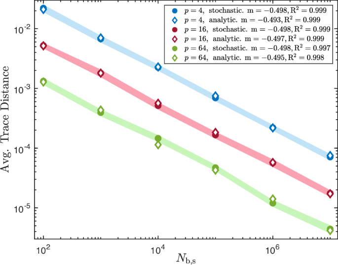
The average trace distance of the gate set is plotted as a function of the number of shots per circuit for various maximum depths of long-sequence circuits. Estimates for stochastically-generated data are displayed with filled markers, whereas those obtained from the closed filtered-noise expressions for the noisy channel based on the Lorentzian PSD (17) are displayed with empty markers. Linear fits are carried out for each set of data. For the shake of clearness, we do not plot the linear fits, but the corresponding slopes are shown in the legend, confirming the expected values around m ≃ −0.5. For the Ornstein-Uhlenbeck simulations, the noise parameters used are τc = 5 ⋅ 10−6s, c = 2 ⋅ 103s−3. To enhance accuracy, we average the process over 100 GST estimates for each data-point. In lighter colours, we plot confidence regions with confidence level γ = 99%.
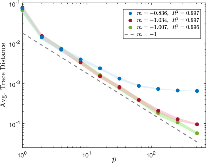
In a similar manner, we have also confirmed the expected 1/p scaling for our parametrised long-sequence GST when computing the average trace distance as a function of the maximum number of repetitions of germs utilized in the resulting circuits. This time, the expected slopes on a log-log scale should be around −1, which also agrees with our numerical results depicted in Fig. 4. Moreover, these results also enable us to confirm the p ≳ 1/Γ1 regime in which errors accumulate considerably, and the accuracy of the GST estimation indeed saturates. The deviation from the 1/p behaviour is not observed in the range of p depths for the green data, as the choice of parameters in this case yields ({Gamma }_{1}^{-1}simeq 1{0}^{5}). In contrasts, the saturation becomes noticeable for data in magenta (({Gamma }_{1}^{-1}simeq 1{0}^{4})) and data in blue (({Gamma }_{1}^{-1}simeq 1{0}^{3})), where one can see how the initial linear slope bends towards a horizontal line when the accumulation of errors forbids getting more information from going to even longer-depth circuits.
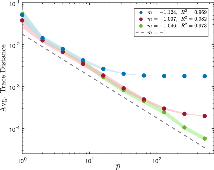
The average trace distance of the gate set is plotted as a function of the maximum number of repetitions of germs utilized in long-sequence circuits for various sets of noise parameters and Nb,s = 103 shots per circuit. This process is repeated for 100 GST estimates at each data-point and then the average values are plotted. Regions in which errors begin to dominate are appreciated. This is in concordance with the (pgtrsim frac{1}{{Gamma }_{1}}) condition anticipated in Subsec. “Selection of parametrized base circuits”. These regions are reflected in the graph by the deviations that magenta and blue data exhibit when compared to the linear function with slope m = −1 (dashed grey), whereas green plot matches the tendency for the whole interval displayed. We do not include values within these regions in the linear fits. For the shake of clearness, we do not plot the linear fits, but the corresponding slopes are shown in the legend. These results confirm the expected slope values m ≃ −1. Parameters for the Ornstein-Uhlenbeck simulations are {τc = 5 × 10⁻⁴s, c = 2 × 10⁴s−3}, {τc = 5 × 10⁻⁴s, c = 2 × 10⁵s−3} and {τc = 5 × 10⁻⁴s, c = 2 × 10⁶s−3} for the green, magenta and blue sets of data, respectively. In lighter colours, we plot confidence regions with confidence level γ = 99%.
We observe here that the accuracies obtained on Figs. 3 and 4 are highly unlikely to be obtained using a characterization method for the PSD. This is due to the fact those schemes rely on assumptions which clash with self-consistency, as already mentioned in subsection. “Filtered-noise parametrization of the gate set”.
As we previously mentioned, we have focused mostly on the Markovian parametrization of the noisy gates in which Γ2(ti) = Δ2(ti) = 0, which is justified when the effects brought up by the non-zero correlation time τc are not too big. As already noted above, our parametrized GST can account for non-Markovian evolutions within each of the gates by simply allowing for Γ2(ti), Δ2(ti) ≠ 0, but not for possible correlations between different gates. Qualitatively, this requires a separation of time scales such that gates are fast enough for the finite τc to play a role, whereas the time lapse between switching off a driving for one gate and switching it on again for the next gate is slow in comparison to τc. This captures noise correlations present in a given gate, assuming that correlations are ‘washed-out’ from one gate to the next.
We can select values of τc for which these non-Markovian effects become visible. We account for this effect by comparing the GST estimates obtained without imposing the approximation Γ2 = Δ2 = 0. As can be observed in Fig. 5, forcing Γ2 = Δ2 = 0 leads to an estimate of a Markovian gate set that becomes less accurate when one reaches a regime in which τc is large enough and non-Markovian effects start to kick in. By allowing for Γ2, Δ2 ≠ 0, the parametrized GST can incorporate such non-Markovian effects, leading to gate set estimates that are more accurate. As pointed out in ref. 57, as one keeps on increasing the correlation time, none of the two parametrizations will be sufficient. In this case, the condition ({tau }_{c}^{3}c,ll, 1) will start to be violated, requiring higher-order terms in the cumulant expansion that underlies the dressed-state master equation and the filtered-noise effective channels. This explains the worsening of both GTS accuracies observed in Fig. 5 as correlation time increases more and more. In any case, we see that the non-Markovian estimate is always better than the Markovian one. We also use a secondary Y-axis to plot the non-Markovianity measure ({{mathcal{N}}}_{{rm{CP}}}(t=pi )) Eq. (36)83,84.
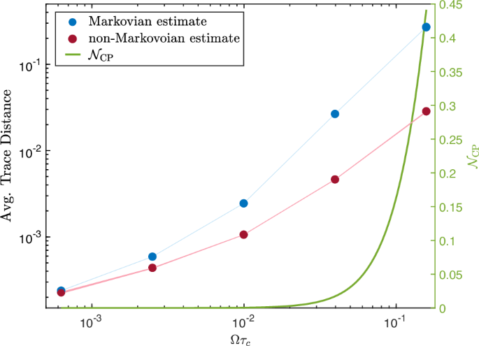
We simulate the non-Markovian GST estimation by relaxing the approximation Γ2 = Δ2 = 0. We then run GST on the numerically-simulated data with both a purely Markovian and a non-Markovian parametrizations. The results from the non-Markovian reconstructions are depicted in magenta, while those from the Markovian reconstructions are shown in blue. The non-Markovian reconstructions effectively capture the short-time correlated effects through the parameters Γ2 and Δ2, thus yielding more accurate tomographic estimates in the regime where τc is larger. In contrast, the Markovian reconstructions fail to capture these effects and exhibit a lower accuracy. In both cases, as τc increases, the condition ({tau }_{c}^{3}c,ll ,1) is relaxed and a worsening of accuracies is observed. We use a secondary Y-axis (green) to plot the non-Markovianity measure ({{mathcal{N}}}_{{rm{CP}}}) Eq. (36) in the same correlation times interval. For this graph, all the reconstructions take circuits of a maximum long-sequence length p = 16 and Nb,s = 105. The parameters for the Ornstein-Uhlenbeck simulations employed are {τc ∈ (5 × 10⁻⁷s, 5 × 10⁻⁴s), c = 1.6 × 10¹¹s−3}. For each data-point, we average over 100 GST estimations. Also, in lighter colours, we plot confidence regions with confidence level γ = 99%.
Comparison with fully-general GST
Once we have checked that our parametrised GST can reproduce the expected scalings in accuracy, and that it can also account for a certain amount of non-Markovian effects, we can finally compare our estimates with those obtained utilizing fully-general GST. As we mentioned in previous subsections, constructing a minimal GST design requires significantly fewer experiments when using our GST based on a reduced set of noise-filtered parameters. This motivates the study presented in Fig. 6, where we plot the average trace distance between the estimated and microscopic gate set as a function of the number of circuits Nc used in the GST estimations. In this case, we assume p = 1 for simplicity, and include the SPAM elements when computing the average trace distance to account for every parameter in the gate set. This allows us to compare the behaviour of parametrized and fully-general GST and, particularly, how the accuracy of the estimation changes as we increase the number of base circuits used in GST.
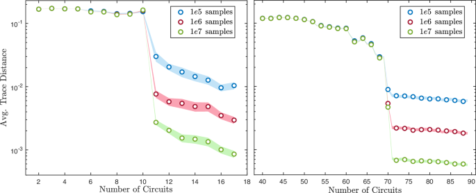
We plot the average trace distance of the gate set as a function of the number of circuits included for both the microscopically-parametrized version of GST (left) and the fully general one (right). In both cases, an improvement in accuracy is observed when the number of non-redundant circuits considered reaches the total number of free parameters in the gate set, which is 67 parameters for the general model, and 11 parameters for the microscopically-parametrized one. The parameters used in these plots are τc = 5 × 10⁻⁴s and c = 2 × 10⁹s−3. We average the process over 100 GST estimates for each data-point. In lighter colors, we plot confidence regions with confidence level γ = 99%.
When the number of circuits is not sufficient to reach IC, Fig. 6 shows that the GST estimation does not work, as the trace distance remains close to that of the initial unitary guess and the actual noisy channels. Since the GST sensitivity to the parameters is very low in this regime of a low-number of circuits, the estimation cannot learn the noisy parameters correctly. As we increase the number of circuits and IC is attained, an abrupt drop in the average trace distance to the actual gate set is observed, signalling that the GST is now accurate. This can be attributed to the fact that every parameter in the gate set is now being optimized when performing the gradient descent of the maximum-likelihood estimation.
We note that the number of circuits at which this drop occurs coincides, for our parametrized model, with the number of free parameters of the noisy gate set NGST = 11 (left panel of Fig. 6). This close agreement is a result of the circuit selection procedure described in subsection “Selection of parametrized base circuits”, which enables us to order circuits according to their sensitivity, and place the first 11 non-redundant elements at the beginning. In contrast, for fully-general GST (right panel of Fig. 6), we observe that the drop in trace distance is only reached further along the circuit axis, requiring thus a larger number of circuits. This should be unsurprising, as the fully-general GST requires estimating NGST = 67 parameters. In contrast to our parametrized GST, where the circuit importance sampling is direct, we rely on the pyGSTi algorithms for fully-general GST to find the minimal set of circuits sufficient to achieve information completeness, according to which 72 different experiments are needed. This number coincides exactly with the point in which trace distance drops in the right panel of Fig. 6.
To give estimates of the total measurement resources required for GST, and compare our parametrized approach to the fully-general one, we finally analyse the average trace distance of the gate set as a function of the total number of shots Nshots. As expected, our parametrized GST provides a significant reduction in the required number of experiments to achieve a target accuracy in comparison to fully-general GST (see Fig. 7). We observe that the accuracy of our parametrized GST outperforms that of fully-general GST by more than an order of magnitude when considering the same total number of shots Nshots. This can be seen when comparing the green data (parametrized GST) with the magenta data (fully-general GST) in Fig. 7. Note that in this figure we are fixing the same maximum depth for the circuits in the long sequence scheme with both models. Thus, the total number of shots Nshots grows by increasing the number of shots per circuit Nb,s employed to compute each frequency fμ,s.
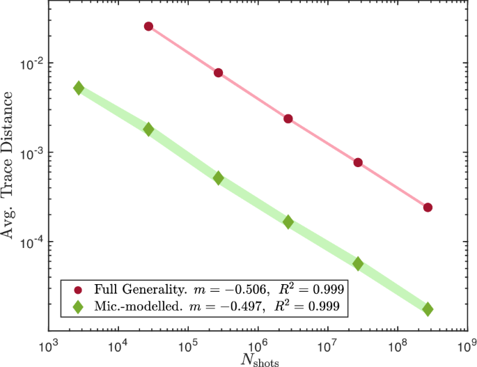
We present the average trace distance of the gate set as a function of the total number of shots used Nshots. In the plot, our microscopically-motivated implementation is depicted in green with diamond markers, while fully general GST implementations is depicted in magenta. It is notable that our parametrized GST achieves a better estimation accuracy even with a significantly reduced total number of circuits required. As expected, accuracy scales as (1/sqrt{{N}_{{rm{shots}}}}) in both cases, as evident from the linear fit slopes. The estimate obtained for Nshots ≃ 103 is only displayed for our parametrized approach, as the number of shots is insufficient to perform GST with the fully-general one. Each plot is generated using p = 16 and the simulation parameters {τc = 5 × 10⁻⁶s, c = 2 × 10³s−3}. We also average the results over 100 iterations to limit the variance and we plot confidence regions with confidence level γ = 99% in lighter colors.
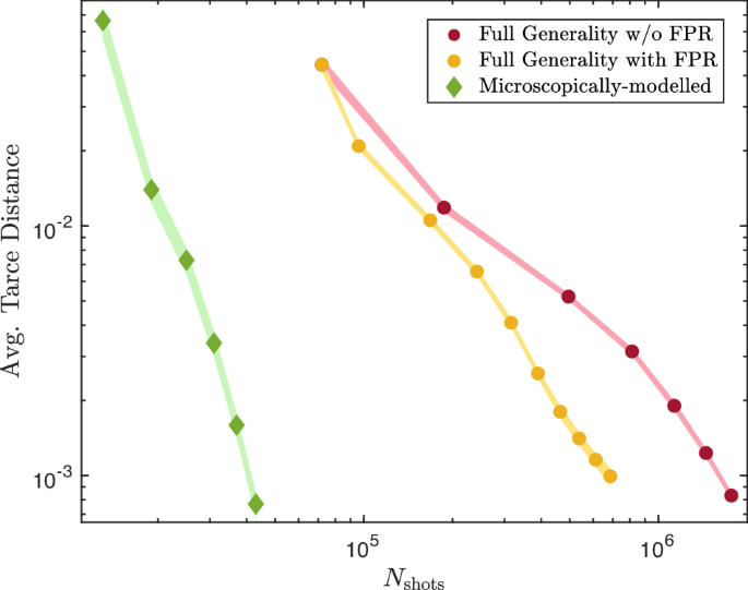
Let us now discuss how the accuracy of the estimation presented in Fig. 7 can be further enhanced. Similar to that figure, Fig. 8 illustrates the average trace distance as a function of Nshots. However, in contrast to Fig. 7, we now more wisely choose to increase Nshots by gradually incorporating deeper circuits in the GST scheme while maintaining the same number of shots Nb,s. This accelerates the improvement in accuracy with the number of shots, as already discussed and evident from Figs. 3 and 4. This aligns with the logic behind the utility of FPR. The fact that one is able to reduce the number of circuits needed to achieve an AC set enables employing the excess of resources not to increase Nb,s (which would generally yield similar results to those without FPR), but to extend circuits further in depth. Consequently, with this expanded range of depths, FPR provides superior results at a constant number of shots. This can be observed when comparing the magenta (no FPR) and the yellow (FPR) curves in Fig. 8. Likewise, our microscopic parametrization does also reduce the number of circuits needed to achieve an AC set. Therefore, akin to FPR, we can allocate the resources more efficiently among deeper circuits. The corresponding plot in Fig. 8 is displayed in green. As can be concluded from this figure, the accuracy enhancement obtained with our parametrized approach is great when proceeding in this way.
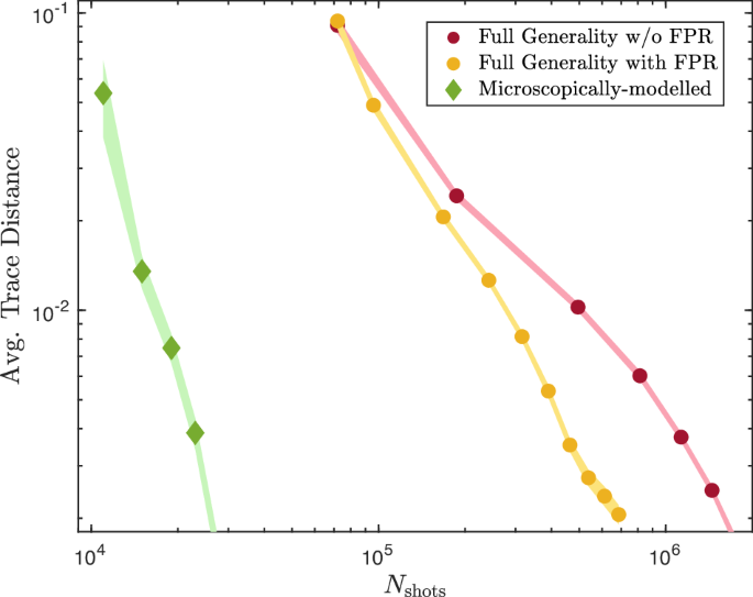
We present the average trace distance of the gate set as a function of the total number of shots used Nshots. In the plot, our microscopically-parametrized GST is depicted in green with diamond markers, while fully general GST implementations are shown in other colors. Specifically, the yellow and magenta plots represent general GST estimations with and without FPR, respectively. Contrary to Fig. 7, we fix the number of shots per circuit, in this case is Nb,s = 103. The total number of shots NShots varies by considering increasingly deeper circuits, ranging in the interval ({p}_{g}in {{{2}^{i}}}_{g = 0}^{9}). It is notable that our parametrized approach achieves much better estimation accuracies at a fixed NShots. Additionally, it is worth mentioning that the improved resource allocation stemming from FPR does also improve the estimations, as evident from the yellow plot. Each plot is generated using the simulation parameters {τc = 5 × 10⁻⁴s, c = 2 × 10⁴s−3}. We also average the results over 100 iterations to limit the variance and plot confidence regions with confidence level γ = 99% in lighter colors.
Inclusion of amplitude noise fluctuations
As extensively detailed in previous sections of this manuscript, our work primarily aims at describing processors subjected to phase noise using the filter-function formalism. Nonetheless, this model can be further extended to additionally account for amplitude or ‘intensity’ fluctuations of the drive. As pointed out in the Methods section, these additional fluctuations are similarly modelled by an stochastic process (delta tilde{Omega }(t)), which describes the variations of the Rabi frequency induced by intensity noise98. Equivalently to the dressed-state master equation description of the pure phase noise evolution, amplitude noise leads to a supplementary filtered integral analogous to those in Eq. (6)
where we have introduced an additional PSD, SΩ, which exclusively describes this process. The new filter function FΩ(ω, t) is explicitly given in Supplementary Subsection II of the supplementary material.
As can be anticipated from Eq. (18), the parameter ΔΓ1(t) neither depends on the driving phases ϕi. Thus, the fact that gates with shared pulse duration are described by the same set of parameters prevails. Consistently with our previous analysis, we employ Fig. 9 as a confirmation that depth-one germs still define an AC set. For this figure, as well as in Fig. 10, we simulate data using two independent stochastic processes under OU niose, i.e. they do not exhibit cross correlations (see the Methods). As usual, we take an average over a sufficiently large number of random trajectories. It is noteworthy that we do not observe an emerging gauge degree of freedom induced by the parameter ΔΓ1(t), therefore, the need of gauge optimization remains absent with this extended model. Using this knowledge and taking advantage of pyGSTi adaptability, we can effortlessly obtain a new figure equivalent to Fig. 8 which does also include amplitude noise fluctuations. As can be expected, the inclusion of two additional parameters to fully characterize the gate set under phase and amplitude noise does not significantly alter the behaviour of the results (see Fig. 10). As a consequence, the discussion concerning Fig. 8 remains accurate.
The average trace distance of the gate set is plotted as a function of the maximum number of repetitions of germs utilized in long-sequence circuits for various sets of noise parameters and Nb,s = 103 shots per circuit. This process is repeated for 100 GST estimates at each data-point and then the average values are plotted. Regions in which errors begin to dominate are appreciated. This is in concordance with the (p,gtrsim ,frac{1}{{Gamma }_{1}}) condition anticipated in Subsec. “Selection of parametrized base circuits” under the substitution Γ1 → Γ1 + ΔΓ1. These regions are reflected in the graph by the deviations that magenta and blue data exhibit when compared to the linear function with slope m = −1 (dashed grey), whereas green plot matches the tendency for the whole interval displayed. We do not include values within these regions in the linear fits, neither the first data-point, which regularly encounters a local minima. For the shake of clearness, we do not plot the linear fits, but the corresponding slopes are shown in the legend. These results confirm the expected slope values m ≃ −1. Parameters for the Ornstein-Uhlenbeck simulations are {τc = 5 × 10⁻⁴s, c = 2 × 10⁴s−3}, {τc = 5 × 10⁻⁴s, c = 2 × 10⁵s−3} and {τc = 5 × 10⁻⁴s, c = 2 × 10⁷s−3} for the amplitude fluctuations in the green, magenta and blue sets of data, respectively. For every simulation, we employ {τc = 5 × 10⁻⁴s, c = 2 × 10⁴s−3} in the phase noise stochastic processes. We recall that phase and amplitude stochastic fluctuations are not cross-correlated. In lighter colors, we plot confidence regions with confidence level γ = 99%.
We present the average trace distance of the gate set as a function of the total number of shots used Nshots. In the plot, our microscopically-parametrized GST is depicted in green with diamond markers, while fully general GST implementations are shown in other colors. Specifically, the yellow and magenta plots represent general GST estimations with and without FPR, respectively. Contrary to Fig. 7, we fix the number of shots per circuit, in this case is Nb,s = 103. The total number of shots NShots varies by considering increasingly deeper circuits, ranging in the interval ({p}_{g}in {{{2}^{i}}}_{g = 0}^{9}). It is notable that our parametrized approach achieves much better estimation accuracies at a fixed NShots. Additionally, it is worth mentioning that the improved resource allocation stemming from FPR does also improve the estimations, as evident from the yellow plot. Each plot is generated using the simulation parameters {τc = 5 × 10⁻⁴s, c = 2 × 10⁴s−3} for both phase and amplitude fluctuations. We recall that these two stochastic processes are not cross-correlated. We also average the results over 100 iterations to limit the variance and plot confidence regions with confidence level γ = 99% in lighter colors.
The inclusion of the amplitude noise fluctuations described is more than a mere generalization of the formalism. As mentioned during the introduction, alongside phase noise, these parameters serve to describe the main sources of errors in trapped-ion devices. For this reason, they are typically referred to as universal noise. This does not mean, however, that our work is not relevant to other quantum processing architectures. Phase, frequency and amplitude noise of the driving agent are common across different platforms. Nonetheless, in each case, a detailed study of the noise sources relevant to the specific architecture has to be carried out.
Discussion
In this work, we have presented a microscopically-motivated GST, which builds on the quantum dynamical map of single-qubit gates subject to phase noise57 to find a compact parametrization of the full gate set in terms of filtered integrals of the noise spectral density. We have generalised this work to parametrise the full gate set, and discussed central differences with respect to the standard fully-general GST, such as the possibility of using single gates as base circuits to achieve amplification completeness. In addition, we showed that germ selection, fiducial pair reduction, and thus the achievement of minimal GST designs can be highly simplified when using this microscopic parametrization. We also highlighted how our approach does not suffer from gauge redundancy, saving computational resources as no gauge-fixing is required, and avoiding reference frame issues when benchmarking the results. We have presented a thorough numerical validation of these arguments considering a specific stochastic model of coloured phase noise, and numerically obtaining maximum-likelihood estimates based on long-sequence GST with numerically-generated data that also includes the effects of shot noise. We have shown that the accuracy of our parametrized long-sequence GST follows the expected scalings with the number of shots and the circuit depth, and demonstrated that our parametrization can account for non-Markovian dynamics during the gates. We have finally showcased the advantages of our parametrized GST with respect to fully-general GST, presenting examples in which a tenfold reduction in the average trace distance can be achieved considering the same number of total measurement shots and circuit depth. We also showed how this reduction can be increased if one allocates the remaining resources in experiments with deeper circuits. Additionally, we showed that these results remain accurate under an extension of the model to include amplitude noise fluctuations.
As an outlook, it would be interesting if future studies assessed if these benefits remain valid when extending to two-qubit gates and crosstalk in an enlarged qubit register, as required for realizing the full potential of quantum computation. On the one hand, the fact that single gates themselves form an amplificationally complete set is something dependent on the specific matrix structure of our parametrized model. An equivalent treatment for entangling gates should be developed to check whether more complex germs are needed for amplification completeness in that case. In order to do that, an extension of the effective quantum dynamical map to model noisy two-qubit gates will be required. Once this is made, we believe that fiducial pair reduction would not longer yield minimal but near-minimal GST designs. We note here that adding entangling gates will still generate disjoint sets of per-germ amplified parameters if the two-qubit gates do also serve as germs. This would facilitate finding good choices for fiducial pairs, but the d −1 independent outcomes of each circuit would still lead to some overhead if each parameter is linked to a single experimental setting, resulting in a more complex combinatorial problem. On the other hand, it could also be the case that some of the new parameters describing the entangling gates are gauge parameters, while the single-qubit gate parameters would remain non-gauge ones. Even in the worst-case scenario in which none of the previous features persists in the two-qubit case, the considerable reduction in the total number of parameters still makes it worth to explore this research avenue. Considering entangling gates in a two-qubit system and also cross-talk in the previous single-qubit gates, the number of parameters needed to characterize this gate set with fully-general GST grows to NGST = 5103. On the contrary, even with no further modelling of the entangling gate, using the present physically-motivated parametrization yields NGST = 423 or NGST = 503 for the Markovian and the non-Markovian estimations respectively, which will be further reduced by a detailed modelling of the noisy entangling gate.
Another interesting question for future research will involve validating our approach with real experimental data, assessing the extent to which our analytical model accurately describes physical quantum devices. The use of this model for trapped-ion QIPs is justified in57 by the fidelity agreement when comparing tomographic results with analytical estimations, but the model can be ultimately extended to include other sources of error, such as intensity noise and spontaneous decay. Once a description of the faulty processes of a device is obtained, it can be further tested using techniques like probabilistic error cancellation (PEC)99, which allows to obtain ideal expectation values in terms of the accessible faulty ones.
Finally, we also note that it would be interesting to extend the description of non-Markovian effects briefly introduced in the final part of subsection “Numerical benchmarks with stochastic noise” beyond the individual gates, such that non-Markovian correlations among the different gates that form the base circuits can be accounted for, which would lead to a fully non-Markovian generalization of GST.
Methods
Coloured phase noise for single-qubit gates
In this section, we describe the central aspects of the phase-noise parametrization of noisy gates employed in the main text, which builds on the recent results for the quantum dynamical map of trapped-ion gates presented in ref. 57. In order to parametrize the full gate set in Eq. (4), we need to generalise this quantum dynamical map to other driving phases, allowing for the SPAM operations required for IC.
Following57, we start by modelling phase noise by a stochastic process (tilde{delta }(t)). For single-qubit gates, the microscopic rotating-frame Hamiltonian for a generic phase reads
where Ω (ϕ) is the Rabi frequency (phase) of the drive, and
includes the frequency (phase) fluctuations (delta tilde{omega }(t),(delta tilde{phi }(t))) described by a specific stochastic process. As a result, the quantum states become stochastic (tilde{rho }(t)=vert tilde{psi }(t)rangle langle tilde{psi }(t)vert), and its Liouville-von Neumann equation which corresponds to a system of stochastic differential equations with multiplicative noise. One can formally derive the equations of motion for the statistical average (rho (t)={mathbb{E}}[tilde{rho }(t)]) by using the Nakajima-Zwanzig approach100,101,102 of projection operators. As discussed in ref. 57, to get a tractable and useful expansion for high-fidelity gates, one utilizes the so-called time-convolutionless methods102,103 in the instantaneous or dressed-state basis64,104,105. By truncating at second order, and setting ϕ = 0, one arrives at a simple time-local master equation that can be expressed in terms of integrals of the covariance
where we assume that ({mathbb{E}}[tilde{delta }(t)]=0). In the dressed-state basis (leftvert pm rightrangle =(leftvert 0rightrangle pm leftvert 1rightrangle )/sqrt{2}), the evolution for the populations reads
where we have introduced the following decay function
This is precisely one of the four parameters which we aim to estimate under GST (see Eq. (6) of the main text). The remaining parameters stem from the evolution of the dressed-state coherences of the density matrix57. This evolution is approximated by a Magnus expansion106 to lowest order, which yields the following integrals
where we have introduced the remaining integrals
These parameters contain all the information that is required in our parametrized GST (see Sec. “Filtered-noise parametrization of the gate set”), where the following combination shall be useful for the parametrization
We can rewrite these parameters in terms of the power spectral density (PSD) of the noise which, when restricting to wide-sense stationary processes (C(t,{t}^{{prime} })=C(t-{t}^{{prime} }))107, is defined by the Fourier transform
This enables one to rewrite the integrals Eq. (24) as
where ({F}_{{Gamma }_{i}}) and ({F}_{{Delta }_{i}}) correspond to the filter functions mentioned during the introduction. In particular, one finds
where we have used the nascent Dirac delta
fulfilling ηϵ(x) → δ(x) as ϵ → 0+, and (mathop{int}nolimits_{-infty }^{infty }{rm{d}}x,{eta }_{epsilon }(x)=1), which clearly acts as a Dirac-type delta filter in the long-time limit. The other filters are defined as follows
where we have introduced
In addition, one also finds
These expression are of particular relevance because the phase-noise PSD can often be accessed experimentally independently of the tomographic characterization, e.g. by a self-heterodyne setup with a reference ultra-stable oscillator in trapped-ion devices56. This would enable to adapt our GST to a specific QIP. For instance, as mentioned in the Results section, the validity of long-sequence GST is limited to the region in which the sequence depth fulfills p ≪ 1/Γ1. Thus, knowing the experimental PSD allows us to give a prior estimation of this region by means of Eq. (6). We note here that an independent experimental estimation of the PSD can be very useful to have a first prediction of the noisy gates. However, we emphasise that this does not undermine our GST tomographic method. Even if the noisy-gate model is fully characterized by the PSD, obtaining this quantity is also prone to errors that propagate onto the gate set. This can lead, depending on the estimation technique, to self-consistency issues as in the case of qubit noise spectroscopy, which extracts the PSD from qubit measurements in an idealized setting in which pulse sequences are error free and even instantaneous108,109,110. We note that this is not self-consistent, as it effectively presumes that some components of the noisy gate set would be perfect for spectroscopy. This limits the accuracy with which the gate set can be reconstructed within this framework, as opposed to our GST proposal.
The former expressions also allow us to explicitly compute the non-Markovianity measure83,84 employed in Sec. “Numerical benchmarks with stochastic noise”. As a notion of quantum non-Markovianity, we use the so-called CP-divisibility
Within this framework, a map is said to be Markovian if one can divide it by the composition of two CPTP maps at each intermediate time. Therefore, acting on the tensor product space ({{mathcal{H}}}_{{rm{S}}}otimes {{mathcal{H}}}_{{rm{S}}}), one can build a non-Markovianity measure on the violation of the CPTP condition for each interval of evolution
where the trace norm is used, (vert {Phi }_{+}rangle =frac{1}{sqrt{2}}(vert 00rangle +vert 11rangle )) and the non-Markovianity measure is defined as ({{mathcal{N}}}_{{rm{CP}}}=mathop{int}nolimits_{0}^{t}{rm{d}}{t}^{{prime} }g({t}^{{prime} })). Explicitly, using the integrals in Eqs. (23) and (25), one gets57
where ({bar{gamma }}_{-}(t)=displaystylefrac{1}{2}{gamma }_{1}(t)-displaystylefrac{1}{2}sqrt{{gamma }_{2}^{2}(t)+{delta }_{2}^{2}(t)}).
Finally, one can use the analytic expressions for the time evolution of the dressed-state density matrix to derive closed expressions for the χϕ(t) matrix of dynamical quantum map. In the Pauli basis, this reads
where the upper and lower blocks can be expressed in terms of the parameters and the Pauli matrices as follows
Note that in contrast to ref. 57, we here present the full χϕ(t) matrix and not only that of the error channel. We also note that, in the absence of noise Γi(t) = Δi(t) = Θ(t) = 0, the process block matrices are simply
and one recovers the perfect gate ({mathcal{E}}(rho )={{rm{e}}}^{-{rm{i}}tfrac{Omega }{2}{sigma }_{x}}rho {{rm{e}}}^{+{rm{i}}tfrac{Omega }{2}{sigma }_{x}}).
For the present work, we need to generalise this derivation for different phase angles ϕ in order to attain IC. For a detailed parametrization of the complete gate set, we refer to Section II of the Supplementary Material, where we also show how intensity noise fluctuations can be incorporated into this formalism.
Responses