Mitigating errors in analog quantum simulation by Hamiltonian reshaping or Hamiltonian rescaling
Introduction
Simulating quantum many-body Hamiltonians is a critical task for exploring complex phenomena in quantum physics. Key applications, including analyzing electronic structures in condensed matter physics1, as well as examining quantum phase transitions between many-body localization and thermalization2,3, rely on accurately evaluating the eigen-energies of quantum many-body systems but pose significant challenges for classical computers. Quantum computers hold the potential to efficiently solve these problems through various phase estimation algorithms4,5,6. A more accessible version for the current noisy intermediate-scale quantum (NISQ) era7 is control-free phase estimation8,9, also known as the many-body spectroscopy technique10,11. This technique determines the eigen-energies of a Hamiltonian by analyzing time series data of expectation values from time-evolved observables. The required Hamiltonian evolution can be implemented in both digital and analog quantum simulators12,13. Digital simulators, which are gate-based and capable of simulating universal Hamiltonians, face challenges such as systematic trotterization errors and increased complexity in circuit compilation. In contrast, analog simulators, tailored for specific tasks, are more straightforward and cleaner but offer limited programmability.
While digital and analog simulators offer distinct advantages, they both grapple with inherent challenges. A crucial concern for these platforms is the mitigation of the effect of noise and operational errors. Digital quantum simulators, combined with quantum error correction (QEC)14,15,16, can achieve fault tolerance in the long term. However, implementing large-scale QEC remains challenging in the near term, despite some experiments reaching the break-even point17,18,19. Analog quantum simulators, due to their limited controllability, lack effective methods to reduce errors. Therefore, developing suitable error cancellation methods for analog simulators, respecting their constraints, is of urgent importance.
One direct method to reduce errors is iterative calibration of the system Hamiltonian through Hamiltonian learning20,21 or quantum benchmarking methods22,23,24,25 that are suitable for analog simulators. In addition to calibration, error can be mitigated at the circuit level through various quantum error mitigation (QEM) methods26. QEM reduces errors by post-processing noisy data and requires significantly fewer quantum resources compared to quantum error correction. Despite the exponential sample scaling with system size27,28,29,30, QEM can enhance computational accuracy in the near term31,32 and potentially reduce the resource overhead of QEC in the long term33. However, most QEM methods are designed for digital quantum computers and require advanced spatial-temporal control. For example, probabilistic error cancellation34 necessitates first characterizing the noise channel of gates and then decomposing ideal gates into noisy ones. Virtual distillation requires many entangling gates between copies of system states35,36,37. The noise resilient phase estimation in ref. 38 requires randomized compiling to tailor the noise into benign type for phase estimation. These methods are currently beyond the capabilities of analog quantum simulators, thus necessitating the development of tailored error mitigation techniques specifically for them.
In this work, we develop two error mitigation techniques for eigen-energy estimation in analog quantum simulators, termed Hamiltonian reshaping and Hamiltonian rescaling. We address the eigen-energy estimation problem using many-body spectroscopy techniques10,11. Both procedures involve preparing an initial state, evolving it under the desired Hamiltonian at varied time intervals, and measuring the expectation values of pertinent observables. The eigen-energies are subsequently deduced from these expectation values using advanced signal processing techniques, such as the matrix pencil method39.
In the Hamiltonian reshaping approach, random unitary operations, ideally Pauli operations, are utilized to modify the original target Hamiltonian into alternative forms that retain the same eigen-energies but alter the eigenstates. By conducting many-body spectroscopy on each modified Hamiltonian, we derive several eigen-energy estimates. An average of these estimates provides an error-mitigated value up to the first order of noise strength.
In the Hamiltonian rescaling approach, we scale the original Hamiltonian by specific factors, resulting in new Hamiltonians that preserve the original eigenstates while altering the eigen-energies. By performing many-body spectroscopy with the rescaled Hamiltonians and adjusted time intervals, we effectively amplify the noise strength. Using the developed formulas, by combining the eigen-energy estimates from rescaled Hamiltonians, we achieve error mitigation up to the first or second order of noise intensity.
It is noteworthy that our Hamiltonian rescaling method bears resemblance to error extrapolation techniques as detailed in refs. 34,40 during the data acquisition phase. However, there is a significant difference in the data processing approaches. Hamiltonian rescaling involves first obtaining eigen-energy estimates for each rescaled Hamiltonian, followed by error mitigation on these noisy estimates. In contrast, error extrapolation focuses on mitigating errors in the expectation values of observables at each time step prior to the extraction of eigen-energy estimates. Additionally, error extrapolation often relies on simplistic functional dependencies between expectation values and noise strength, such as polynomial or exponential relationships. These do not adequately capture the true relationship–a sum of complex exponential functions. As such, error extrapolation tends to offer less mitigation efficacy in this context compared to our Hamiltonian rescaling method, a conclusion supported by numerical experiments.
Results
Review of many-body spectroscopy technique
Before discussing error mitigation, we first review a protocol designed to evaluate the eigen-energy differences of a given Hamiltonian using analog quantum simulators. This technique is commonly referred to as many-body spectroscopy10,11. Additionally, this protocol has been extended to digital quantum simulators as robust phase estimation8,9.
Consider an analog quantum simulator with n effective qubits, where the goal is to solve the eigenvalue problem of an effective Hamiltonian H that can be operated on the simulator. The eigenvalue problem of H is expressed as (Hvert {phi }_{j}rangle ={E}_{j}vert {phi }_{j}rangle), with the set of eigenstates and corresponding eigenvalues denoted as ({vert {phi }_{j}rangle ,{E}_{j}}). Let S be the set of indices j such that j ∈ S. Now, consider an arbitrary observable O. By preparing the initial state (vert psi rangle ={sum }_{jin S}{c}_{j}vert {phi }_{j}rangle) and subsequently evolving it under the Hamiltonian H for a time duration t, the expectation value (langle Orangle (t)) can be experimentally measured. The Fourier spectrum of (langle Orangle (t)) reveals information about the eigenvalue differences El − Em (where l, m ∈ S). It can be demonstrated that the positions of the peaks in this spectrum correspond to these eigenvalue differences, thus enabling the solution of the eigenvalue problem. We proceed to present a detailed experimental protocol for general cases in four steps.
-
1.
Prepare an initial state (vert psi rangle ={sum }_{jin S}{c}_{j}vert {phi }_{j}rangle), which includes the eigenstates of interest.
-
2.
Evolve the quantum state with Hamiltonian H over different time: 0, ΔT, 2ΔT, … , (L − 1)ΔT, where we set time interval (Delta T ,<, frac{pi }{max (| {E}_{l}-{E}_{m}| )}).
-
3.
Measure the observable O after each experiment to obtain time-series data (leftlangle Orightrangle (0)), (leftlangle Orightrangle (Delta T)), ⋯ , (leftlangle Orightrangle ((L-1)Delta T)).
-
4.
Retrieve the information of eigen-energy differences EbaΔT, where Eba = Eb − Ea are the energy differences between (leftvert {phi }_{b}rightrangle) and (leftvert {phi }_{a}rightrangle), from time-series data (leftlangle Orightrangle (kDelta T)) by signal processing methods, such as the matrix pencil method39.
The protocol is illustrated in Fig. 1a. The key steps of the proof are briefly summarized below. The state at the time kΔT is
Then the expectation value of the operator O is
Thus, the expectation values (langle Orangle (kDelta T)) is a function of the variable k, which is composed of some oscillating functions. The oscillating frequencies (El − Em)ΔT are relevant to the eigen-energy differences, which can be retrieved by some signal-processing methods.
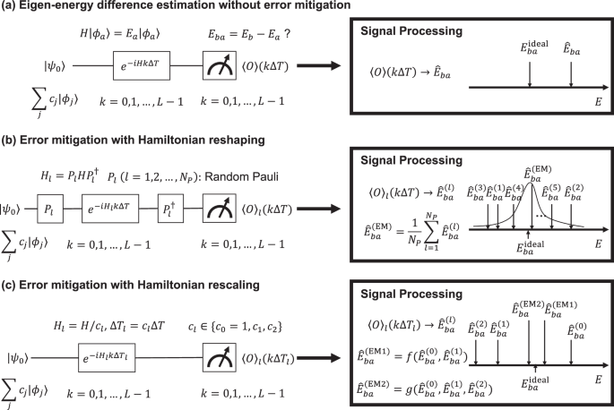
a The many-body spectroscopy technique estimates the eigen-energy differences of the Hamiltonian H. A quantum state (scriptstyleleftvert {psi }_{0}rightrangle ={sum }_{j}{c}_{j}leftvert {phi }_{j}rightrangle) is prepared, representing a superposition of Hamiltonian eigenstates. The state is evolved over time intervals kΔT (where k = 0, 1, …, L − 1), and the observable O is measured to obtain the time-series signal (left{langle Orangle (kDelta T)right}). This signal is analyzed using methods like the matrix pencil method to determine the oscillating frequencies and corresponding eigen-energy differences. Noise in the Hamiltonian evolution causes deviations in the estimated energy differences ({hat{E}}_{ba}). We consider both the unitary noise caused by error Hamiltonian H(1) and the stochastic noise induced by the dissipator ({mathcal{D}}[cdot ]) as defined in Eq. (1). b In Hamiltonian reshaping, random Pauli operations Pl are applied to reshape the original Hamiltonian H into new Hamiltonians ({H}_{l}={P}_{l}H{P}_{l}^{dagger }). For each reshaped Hamiltonian Hl, the many-body spectroscopy technique is employed to estimate the eigen-energy difference ({hat{E}}_{ba}^{(l)}), with the initial state and measurement appropriately transformed. The averaged eigen-energy estimates ({hat{E}}_{ba}^{(l)}) from different reshaped Hamiltonians yield results that match the ideal values up to the first order of noise strength, assuming weak noise and first-order perturbation theory. c In Hamiltonian rescaling, the energy scale of the original Hamiltonian H is adjusted to obtain new Hamiltonians Hl = H/cl. For each rescaled Hamiltonian Hl, the many-body spectroscopy technique is used to estimate the eigen-energy difference ({hat{E}}_{ba}^{(l)}), with the rescaled time interval ΔTl = clΔT. By applying the developed formulas in Eqs. (16) and (19), eigen-energy estimation errors can be mitigated up to the first or second order of noise strength using these ({hat{E}}_{ba}^{(l)}).
The expectation value of the operator O typically includes many eigen-energy differences, which complicates their retrieval. Therefore, it is necessary to limit the number of eigen-modes present in the data by selecting appropriate initial states and observables9,38,41. Suppose we aim to evaluate the energy differences between the eigen-states (vert {phi }_{b}rangle) and (vert {phi }_{a}rangle). We can choose the initial state as (vert {psi }_{0}rangle =frac{1}{sqrt{2}}(vert {phi }_{a}rangle +vert {phi }_{b}rangle)) and a non-Hermitian measurement operator as (2vert {phi }_{b}rangle langle {phi }_{a}vert), which can be decomposed into a complex superposition of Hermitian operators. In this configuration, the data ({langle 2vert {phi }_{b}rangle langle {phi }_{a}vert rangle (kDelta T)}) will only contain information about Eba = Eb − Ea, thereby facilitating the efficient retrieval of the specific energy difference. If one of the eigen-energies is known, the absolute value of the other eigen-energy can be computed. The state preparation and measurement process can be realized through adiabatic quantum evolution from an initial Hamiltonian, whose eigen-states are readily prepared, to the target Hamiltonian H, following the procedures outlined in refs. 41,42,43. In addition to the adiabatic method, certain Hamiltonians offer natural choices for initial states and observables, such as excitation-conserving Hamiltonians. For these Hamiltonians, we can prepare the initial state as an equal superposition state of zero and single excitation states11,44,45,46,47. This approach ensures that the data will exclusively reflect the energy differences between the eigen-states in single excitation subspace and the zero excitation state.
The effect of noise
In real quantum devices, noise is unavoidable and can affect the results of quantum algorithms. This section analyzes the impact of noise on many-body spectroscopy technique using matrix perturbation theory, under the assumption that the noise strength is weak relative to the energy scale of the target Hamiltonian. Additionally, it is assumed that the noise is time-independent.
Without loss of generality, we assume that the evolution of the noisy quantum simulator is described by the following Lindblad master equation:
where Hexp = H + H(1) is the effective Hamiltonian in the experiment, H(1) represents the systematic error of the Hamiltonian (assumed to be small), ({mathcal{D}}[cdot ]=frac{1}{2}{sum }_{k}(2{L}_{k}cdot {L}_{k}^{dagger }-{L}_{k}^{dagger }{L}_{k}cdot -cdot {L}_{k}^{dagger }{L}_{k})) is the dissipator (Lk are Lindblad operators), and ({mathcal{L}}) is the Liouvillian super-operator. Denote (widetilde{{mathcal{D}}}[cdot ]=-i[{H}^{(1)},cdot ]+{mathcal{D}}[cdot ]) as the noise super-operator such that
Consider the eigenvalue problem of the Liouvillian super-operator. If the noise strength is weak ((| widetilde{{mathcal{D}}}| ll | [H,cdot ]|)), (widetilde{{mathcal{D}}}) can be considered as a small perturbation. The right eigenvalues and eigen-states of the Liouvillian super-operator before perturbation are the same as those of the super-operator − i[H, ⋅], which are (left{i({E}_{b}-{E}_{a})right}) and (left{leftvert {phi }_{a}rightrangle leftlangle {phi }_{b}rightvert right}). Consider the non-degenerate first-order perturbation theory, the eigenvalues of the Liouvillian super-operator are
with the corresponding eigen-operators Mab such that ({mathcal{L}}[{M}_{ab}]={Lambda }_{ab}{M}_{ab}). The density matrix can be expanded by the set of eigen-operators Mab
Substituting the equation above into the master equation we obtain
so that
where the initial time is set as zero. Then the expectation value of the operator O after time kΔT is
where we define
and
This result indicates that expectation value (leftlangle Orightrangle (kDelta T)) can be expressed as a sum of damped oscillation modes. Signal processing techniques can still be employed to extract the phase information δϕab, thereby allowing for the estimation of the eigen-energy difference Eba = Eb − Ea. This protocol is resilient to state preparation and measurement (SPAM) errors, as these errors affect only the value of Cab and do not influence the phase δϕab.
However, from Eq. (10), we observe that the eigen-energy estimate ({hat{E}}_{ba}=delta {hat{phi }}_{ab}/Delta T) is biased due to noise, unless (langle {phi }_{a}vert widetilde{{mathcal{D}}}[vert {phi }_{a}rangle langle {phi }_{b}vert ]vert {phi }_{b}rangle in {mathbb{R}}). A sufficient condition for an unbiased estimate, up to the first order of noise strength, is that the Lindblad operators Lk are Hermitian and that the systematic error H(1) = 0. This condition reflects the requirements outlined in our previous work38. However, ref. 38 necessitates randomized compiling to tailor general noise to the desired type, a technique that is challenging to implement in analog quantum simulators due to their limited control capabilities. Therefore, there is a need to develop appropriate error mitigation methods specifically tailored for analog simulators.
We now introduce two error mitigation strategies tailored for the Hamiltonian eigen-energy estimation problem in analog quantum simulators: Hamiltonian reshaping and Hamiltonian rescaling.
Hamiltonian reshaping strategy
The Hamiltonian reshaping technique involves applying random unitary transformations to the original target Hamiltonian, generating new Hamiltonians that retain the same eigen-energies while possessing different eigenstates. This approach allows the eigen-energy estimates derived from these transformed Hamiltonians to be influenced by distinct aspects of noise. We show that averaging these estimates leads to an unbiased eigen-energy estimate, accurate up to the first order in noise strength.
Consider a random unitary operation U from a set G, which transforms the Hamiltonian H into HU = UHU†. The eigenvalues of HU remain identical to those of H, while its eigenstates transform to (Uvert {phi }_{j}rangle). Using the many-body spectroscopy technique in the previous section, we can estimate the phase (delta {phi }_{ab}^{(U)}) in the time interval ΔT for HU between the states (Uvert {phi }_{b}rangle) and (Uvert {phi }_{a}rangle)
The eigen-energy estimate ({hat{E}}_{ba}^{(U)}=delta {hat{phi }}_{ab}^{(U)}/Delta T) for each Hamiltonian HU is biased. However, if we average these eigen-energy estimates from different HU with U ∈ G, then
We can design a set G to ensure the condition
and in this case, the estimated result of Eba after mitigation is
which is unbiased up to the first order of noise strength.
There are numerous sets G that satisfy the condition outlined in Eq. (13), including the Clifford group and the Pauli group. However, when the Hamiltonian is expanded in the Pauli basis, the Clifford-transformed Hamiltonians exhibit Pauli terms that differ significantly from those of the original Hamiltonian, thereby complicating practical experimental implementation. Conversely, a Pauli-transformed Hamiltonian retains the same Pauli terms as the original Hamiltonian, albeit with opposite signs sometimes. Utilizing the properties of Pauli twirling48, we demonstrate that if G comprises the set of n-qubit Pauli operations and H is a Hamiltonian in an n-qubit quantum system, the condition necessary for error mitigation, as specified in Eq. (13), is satisfied for a general noise channel (widetilde{{mathcal{D}}}) (see “Methods”). We refer to this method as Hamiltonian reshaping, which is also employed in Hamiltonian learning20 and noise tailoring49. This approach is illustrated in Fig. 1b.
The Hamiltonian reshaping can be effectively implemented in typical analog quantum simulators by selecting an appropriate set of random unitary operators that align with the constraints of the target system. As previously mentioned, the preferred choice for G is a set of Pauli operations, which only alters the sign of Pauli terms in a Hamiltonian. Generally, the sign of local Pauli operators can be altered by adjusting the detuning and phase of the control pulse. The interaction Hamiltonian terms often consist of weight-2 Pauli operators, such as X ⊗ X, Z ⊗ Z and exchange interaction X ⊗ X + Y ⊗ Y. Various techniques are available for modifying their signs in superconducting circuits50,51,52, trapped ions53,54,55, and neutral atoms56,57,58,59. However, it is important to note that certain Pauli operators in the protocol transform the exchange interaction X ⊗ X + Y ⊗ Y to X ⊗ X − Y ⊗ Y, which is usually unattainable in experimental settings. In such cases, it is necessary to select a smaller set of Pauli operators rather than the full Pauli group to reshape the Hamiltonian while preserving the interaction terms. A particular choice is the set (left{{I}^{otimes n},{X}^{otimes n},{Y}^{otimes n},{Z}^{otimes n}right}), where each element commutes with the exchange interactions, thereby preserving these interactions. Although this smaller set of Pauli operators (left{{I}^{otimes n},{X}^{otimes n},{Y}^{otimes n},{Z}^{otimes n}right}) may not fully mitigate errors arising from general noise, it can mitigate errors due to any local noise. Moreover, reshaping with the full Pauli group suffers from statistical errors due to the limited samples of Pauli operations. Consequently, the smaller set (left{{I}^{otimes n},{X}^{otimes n},{Y}^{otimes n},{Z}^{otimes n}right}) performs better when dealing with local noise. An even smaller set, (left{{I}^{otimes n},{X}^{otimes n}right}), is effective in mitigating errors due to amplitude damping noise and local Z unitary errors, which are the most prevalent types of noise in quantum systems, as illustrated in Fig. 4.
We summarize the Hamiltonian reshaping strategy as follows:
-
Step 1: Generate a set of random Hamiltonians HU = UHU†, reshaped by a random unitary operation U ∈ G. Here, G is preferably chosen as a set of Pauli operations.
-
Step 2: For each reshaped Hamiltonian HU, estimate ({hat{E}}_{ba}^{(U)}) using the many-body spectroscopy technique.
-
Step 3: Compute the error mitigated estimate of energy difference Eba by applying Eq. (14).
Hamiltonian rescaling strategy
The Hamiltonian rescaling method, on the other hand, involves adjusting the energy scale of the target Hamiltonian, producing a series of Hamiltonians with identical eigenstates but differing eigen-energies. Correspondingly, we modify the time scale to preserve the ideal phase evolution at each time interval, effectively amplifying the impact of noise on the eigen-energy estimates. By combining the estimates from both the original and rescaled Hamiltonians using appropriately developed formulas, we can mitigate errors up to the first or second order in noise strength.
Inspired by ref. 34, we develop an error mitigation strategy based on the concept of Hamiltonian rescaling. Notably, our approach distinctly diverges from the conventional zero-noise extrapolation methods described in refs. 34,40, aiming to offer a unique perspective on reducing quantum errors.
First, we obtain the estimate ({hat{E}}_{ba}^{(0)}={hat{E}}_{ba}=delta {hat{phi }}_{ab}/Delta T) from the original Hamiltonian using the many-body spectroscopy technique. Next, we consider the rescaled Hamiltonian ({H}^{{prime} }(t)=frac{1}{c}H(t/c)) where c ∈ (1, + ∞), let (Delta {T}^{{prime} }=cDelta T), and obtain the corresponding (delta {phi }_{ab}^{{prime} }) using the same protocol. Thus, we have
Here, we assume the dissipator is time-translation invariant, so that the noise effect does not change if we only rescale the strength of the Hamiltonian. This assumption, also made in refs. 34,60, is crucial for experimentally controlling the noise strength in the zero-noise extrapolation method34,40. Nevertheless, our objective differs from this approach, as we aim to directly counteract the effects of noise rather than merely extrapolating to a zero-noise scenario. Although the fluctuations of T1 and T2 errors exist over large time scales in real experiments, if measurements for different rescaling factors for the same evolution time are performed in quick succession, this assumption can be justified according to the experiment in ref. 60.
We define ({hat{E}}_{ba}^{(1)}=delta {hat{phi }}_{ab}^{{prime} }/Delta {T}^{{prime} }) as a biased estimator for Eba/c. Combining Eqs. (10) and (15), we obtain the error mitigated energy estimate
It should be noted that the above equation does not explicitly depend on noise factors; hence, this strategy effectively mitigates the impact of noise. It is important to note that the parameter c must not be excessively large, as (widetilde{{mathcal{D}}}[cdot ]) is intended to act as a minor perturbation in comparison to (-ileft[frac{1}{c}H(t/c),cdot right]), ensuring the effective application of perturbation theory. Furthermore, a larger c reduces the estimation error of Eba, as this is directly proportional to (frac{c}{c-1}).
We now examine the second-order corrections to the non-degenerate eigenvalues of the Liouvillian operator ({mathcal{L}}). The Liouvillian is defined as ({mathcal{L}}[cdot ]=-i[H,cdot ]+widetilde{{mathcal{D}}}[cdot ]), with the left and right eigenvectors of the unperturbed part − i[H, ⋅] being (left{leftvert {phi }_{a}rightrangle leftlangle {phi }_{b}rightvert right}), corresponding to eigenvalues (left{i{E}_{ba}right}). The outcomes of the second-order corrections can be derived using eigenvalue perturbation theory61:
To effectively implement error mitigation, at least two rescaling factors, c1 and c2, are required. Under this scheme, we can extract estimates ({hat{E}}_{ba}^{(l)}=delta {hat{phi }}_{ab}^{(l)}/Delta {T}_{l}) by utilizing the rescaled Hamiltonian Hl = H/cl, where the corresponding time interval is given by ΔTl = clΔT. As
we can mitigate the error up to the second order of noise strength by
We note that this Hamiltonian rescaling strategy is different from the Richardson extrapolation method in ref. 34. They both use the experiment data before and after rescaling the Hamiltonian, but process the experiment data with different methods (see Fig. 5a). Our Hamiltonian rescaling strategy is designed to address the damped oscillation relationship described by Eq. (7), a feature that the Richardson extrapolation method cannot fully capture. Consequently, our approach provides a more customized solution for addressing the complexities intrinsic to the many-body spectroscopy problem. Furthermore, this strategy is experimentally viable, as the coefficients of the effective Hamiltonian can be modified using the same method employed in Hamiltonian reshaping.
We summarize this strategy into three steps:
-
Step 1: Choose c1, c2 > 1.
-
Step 2: Estimate ({hat{E}}_{ba}^{(0)}=frac{delta {hat{phi }}_{ab}}{Delta T}), ({hat{E}}_{ba}^{(1)}=frac{delta {hat{phi }}_{ab}^{(1)}}{Delta {T}_{1}}), and ({hat{E}}_{ba}^{(2)}=frac{delta {hat{phi }}_{ab}^{(2)}}{Delta {T}_{2}}) by many-body spectroscopy technique with the original and rescaled Hamiltonian H(t) = H, ({H}_{1}(t)=frac{1}{{c}_{1}}Hleft(frac{t}{{c}_{1}}right)), and ({H}_{2}(t)=frac{1}{{c}_{2}}Hleft(frac{t}{{c}_{2}}right)).
-
Step 3: Mitigate the energy estimation error by Eq. (19).
Numerical results
We demonstrate our error mitigation strategies with numerical experiments, performed using the simulation package QuTiP62,63. We consider a Hamiltonian defined on a qubit ring model, which is a modification from the model discussed in ref. 64:
Here, (leftlangle i,jrightrangle) indicates that i and j are the nearest neighbors on a qubit ring. The dissipator of the dynamics is given by
where ({L}_{k}=sqrt{kappa }(ileftvert 0rightrangle {leftlangle 0rightvert }_{k}+leftvert 1rightrangle {leftlangle 1rightvert }_{k})otimes {{bf{I}}}_{{rm{others}}}) for k = 1, …, n, and κ represents the strength of the noise. Additionally, we consider a systematic error Hamiltonian ({H}^{(1)}=kappa beta mathop{sum }nolimits_{j = 1}^{n}{Z}_{j}). In this study, we do not consider measurement error and statistical error due to finite shots.
We randomly choose 100 pairs of eigen-states (a, b) to demonstrate our error mitigation strategies in statistics. For each pair of (a, b), we prepare the initial state (frac{1}{sqrt{2}}(vert {phi }_{a}rangle +vert {phi }_{b}rangle)), evolve the state with noise and obtain expectation values (leftlangle 2leftvert {phi }_{b}rightrangle leftlangle {phi }_{a}rightvert rightrangle (kDelta T)) where k = 0, 1, ⋯ , L − 1. The ideal results of eigen-energy differences Eba = Eb − Ea are given by exact diagonalization. To improve the estimation accuracy, we use the matrix pencil method39 instead of discrete Fourier transform to retrieve the oscillation frequency (see “Methods”) from the signal (left{leftlangle 2leftvert {phi }_{b}rightrangle leftlangle {phi }_{a}rightvert rightrangle (kDelta T)right}) and estimate Eba. We note that the Hamiltonian reshaping and Hamiltonian rescaling methods also work well when the initial state contains multiple eigenstates (see Supplementary Information).
First, we demonstrate the impact of the Hamiltonian reshaping error mitigation strategy. We apply 100 random Pauli operations to generate reshaped Hamiltonians and average their eigen-energy estimates to achieve error mitigation. Considering local error in our settings, we also assess the error mitigation effect using reshaped Hamiltonians with a smaller set (left{{I}^{otimes n},{X}^{otimes n},{Y}^{otimes n},{Z}^{otimes n}right}). The mitigated relative estimation error and the distribution of relative error for each eigenvalue difference are presented in Fig. 2. Our findings indicate that this strategy efficiently reduces the relative estimation error statistically.
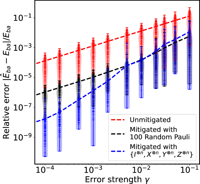
The eigen-energy differences Eba = Eb − Ea for 100 randomly chosen pairs of eigenstates (a, b) are estimated. We consider the Hamiltonian in Eq. (20) with parameters n = 6, νz = 4, νx = 1, and J = 4. The Lindblad operators are assumed to be ({L}_{k}=sqrt{kappa }(ileftvert 0rightrangle {leftlangle 0rightvert }_{k}+leftvert 1rightrangle {leftlangle 1rightvert }_{k})otimes {{bf{I}}}_{{rm{others}}}) for k = 1, …, n, and the error Hamiltonian is ({H}^{(1)}=kappa beta mathop{sum }nolimits_{j = 1}^{n}{Z}_{j}). Parameters are set to β = 0.01, ΔT = 0.0001, and L = 2000. For each numerical experiment, κ = γ∣Eba∣ is used to reflect the relative error strength. The red line represents the average estimated relative error before error mitigation. Error mitigation is performed using 100 Pauli reshaped Hamiltonians, with the black line showing the average result after mitigation. The blue line indicates the mitigation result using reshaped Hamiltonians with (left{{I}^{otimes n},{X}^{otimes n},{Y}^{otimes n},{Z}^{otimes n}right}). When the error rate is small, this method performs better due to reduced statistical errors, as discussed in “Results“. The violin plot illustrates the distribution of relative errors before or after mitigation for these 100 Eba values.
Secondly, we demonstrate the effectiveness of Hamiltonian rescaling in mitigating errors. The results presented in Fig. 3 show that our error mitigation strategy is effective under conditions of weak noise, with the second-order correction providing better mitigation than the first-order correction. When the noise is strong, the mitigated error may exceed the unmitigated error because perturbation theory breaks down in this regime, rendering the error mitigation methods ineffective. In the strong noise regime, the first-order method can outperform the second-order estimate because experiments with a large rescaling factor c may fall outside the perturbative regime, where perturbation theory is less effective, while experiments with smaller rescaling factors remain within a regime where perturbation theory still holds.
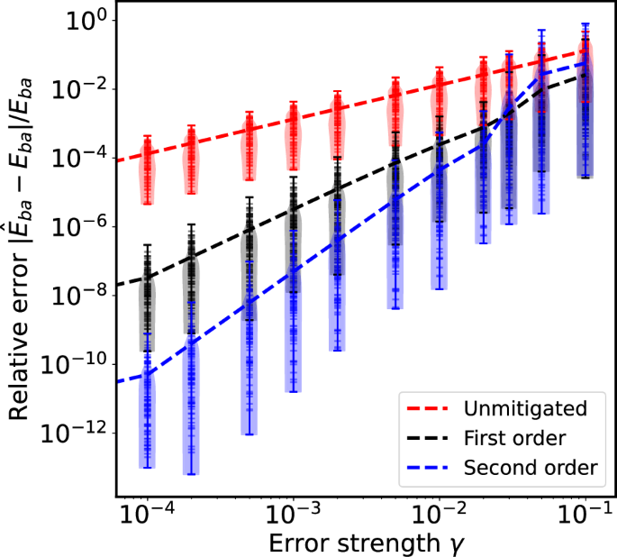
The same 100 pairs of eigen-states (a, b) as those in Fig. 2 are considered. We choose scale factors c1 = 2 and c2 = 1.5. The other settings are the same as that in Fig. 2. The dashed lines show the relative error of these 100 eigenvalue differences in average, and the violin plot shows their corresponding distribution. These results demonstrate that our strategy significantly mitigates the relative error, with the second-order correction providing superior accuracy compared to the first-order correction. In the log-log scale plot, the slope of the unmitigated line is approximately 1, consistent with Eq. (10). The slope of the first-order correction line is close to 2, and that of the second-order correction is approximately 3, indicating effective mitigation of errors up to the first and second orders.
It has been observed that more efficient methods for Hamiltonian reshaping can be developed for specific types of noise, and we numerically evaluate such a method here. When the dominant noise type in the quantum simulator is identified, it becomes feasible to design a reduced set G within the Hamiltonian reshaping strategy, optimized to counteract this particular noise. For example, if the stochastic noise is amplitude damping with Lindblad operators ({L}_{k}=sqrt{kappa }leftvert 0rightrangle {leftlangle 1rightvert }_{k}otimes {{bf{I}}}_{{rm{others}}}), for k = 1, …, n, and the systematic error in the Hamiltonian is represented by ({H}^{(1)}=kappa beta mathop{sum }nolimits_{j = 1}^{n}{Z}_{j}), then setting (G=left{{{bf{I}}}^{otimes n},{X}^{otimes n}right}) is advantageous. This configuration is justified because ({L}_{k}^{dagger }={X}^{otimes n}{L}_{k}{X}^{otimes n}), and (left{{H}^{(1)},{X}^{otimes n}right}=0) in this scenario. We test the tailored strategy with a transverse field XX model:
The results in Fig. 4 show that the Hamiltonian reshaping strategy tailored for the specific yet practical type of noise can effectively mitigate the error.
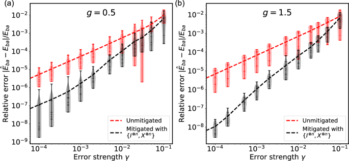
The figure demonstrates the impact of T1-type noise on a model Hamiltonian H = − ∑iXi − ∑iYi − g∑〈i, j〉XiXj, with systematic error ({H}^{(1)}=kappa beta mathop{sum }nolimits_{j = 1}^{n}{Z}_{j}), and the effectiveness of a Hamiltonian reshaping technique. T1 noise is modeled by the Lindblad operator ({L}_{k}=sqrt{kappa }leftvert 0rightrangle {leftlangle 1rightvert }_{k}otimes {{bf{I}}}_{{rm{others}}}), where k = 1, …, n and n = 6 qubits. The relative error strength is γ = κ/∣Eba∣. Parameters are set as β = 0.01, ΔT = 0.0001, L = 2000. Panels a and b illustrate that the estimation of the energy difference Eba is affected by noise in a manner that varies with the interaction strength g. The Hamiltonian reshaping method using (left{{{bf{I}}}^{otimes n},{{bf{X}}}^{otimes n}right}) provides effective mitigation under these conditions.
We also compare the mitigation effect of Hamiltonian rescaling strategy with Richardson extrapolation method34 in Fig. 5. The standard Richardson extrapolation method mitigate the estimation error of the expectation value of observable. First, with the noisy estimates ({leftlangle Orightrangle }_{l}(kDelta {T}_{l})) from rescaling factors cl, one can get error mitigated expectation value of observable ({leftlangle tilde{O}rightrangle }_{0}(kDelta {T}_{0})) at each time. Then one can retrieve the energy difference with the mitigated observable by matrix pencil method. The mitigated estimate of observable expectation value is given by
with single rescaling factor c1 and
with two rescaling factors c1 and c2. The numerical results indicate that our Hamiltonian rescaling strategy outperforms the standard Richardson extrapolation method, as anticipated before.
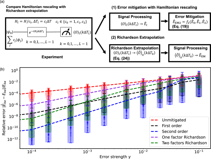
Although both the Hamiltonian rescaling strategy and Richardson extrapolation utilize the same experimental data, they differ fundamentally in their approach to error mitigation. a(1) In our Hamiltonian rescaling strategy, the signal from the experimental data is first processed to estimate the eigenvalue differences, followed by the application of the error mitigation procedure. a(2) In contrast, the Richardson extrapolation method mitigates the signal corresponding to the mean value of the measurement observable before estimating the eigenvalue differences using the mitigated signal. b Numerical comparison of these two strategies under the conditions described in Fig. 3. Given that the 〈O〉 vs. t signal behaves as a summation of damped oscillation modes, as discussed in “Results”, our Hamiltonian rescaling strategy demonstrates higher efficiency compared to the standard Richardson extrapolation, as shown in panel b. We note that the sample complexity of the Hamiltonian rescaling strategy is slightly higher than that of the Richardson extrapolation method (see Supplementary Information).
Complexity analysis
The sample complexity of our error mitigation strategies can be obtained by analyzing the uncertainty in the mitigated eigen-energy estimation, which is intrinsically linked to the unmitigated estimates of eigen-energy difference. This relationship is fundamentally governed by the Fourier analysis underlying the many-body spectroscopy protocol. When employing a discrete Fourier transform to analyze the Fourier spectrum, the precision of the frequency determination is inherently limited by 2π/L. Consequently, the uncertainty in the energy difference is bounded by 2π/(LΔT).
To refine our frequency analysis, we consider the matrix pencil method and the least squares regression method to accurately retrieve Fourier frequencies. Both methods exhibit similar sample complexity, and we will employ least squares regression to analyze this complexity. Let yk = 〈O〉(kΔT) for k = 0, 1, …, L − 1, and denote ωj as the Fourier frequencies corresponding to the list 〈O〉(kΔT). Assuming the relationship between yk and k can be modeled as a sum of damped oscillation modes, we express this as: ({hat{y}}_{k}=mathop{sum }nolimits_{j = 1}^{M}{C}_{j}{r}_{j}^{k}{e}^{i{omega }_{j}k}), where Cj, rj, and ωj are parameters to be determined by regression, and M is the number of significant modes discerned, ideally from the discrete Fourier transform results. The accuracy of this model increases with L, recommending L ≫ Nm (where Nm denotes the number of modes involved) and at least L≥Nm. The optimization is performed over the cost function: (ell =mathop{sum }nolimits_{k = 0}^{L-1}{N}_{k}| {y}_{k}-{hat{y}}_{k}{| }^{2}) where Nk indicates the number of repetitions of the quantum circuit to acquire yk. Optimization seeks to minimize the multi-variable function ℓ(Cj, rj, ωj) to obtain optimal ωj so that δϕab/ΔT can be retrieved by ωj/ΔT. The regression process can be executed using any multi-variable optimization technique on a classical computer. While the cost function is typically non-convex, we can initialize the parameters using results obtained from discrete Fourier transform or other signal processing techniques that identify Fourier frequencies.
The uncertainty associated with this method, as well as the estimation of sample complexity for the many-body spectroscopy protocol, are derived similarly to the approach detailed in Appendix D3 of ref. 44. For further elaboration, readers can refer to Supplementary Information, which provides a derivation. The relationship between the uncertainty of the phase estimation result and the noise strength (| widetilde{{mathcal{D}}}|) is determined by
where ({sigma }_{{omega }_{alpha }}) is the standard deviation of estimation result of the damped oscillation frequencies which characterize the uncertainty and ({r}_{alpha } sim {e}^{{rm{Re}}leftlangle {phi }_{a}rightvert widetilde{{mathcal{D}}}[leftvert {phi }_{a}rightrangle leftlangle {phi }_{b}rightvert ]leftvert {phi }_{b}rightrangle Delta T}={e}^{-{d}_{ab}| widetilde{{mathcal{D}}}| Delta T}) from Eq. (7) (where ({d}_{ab}=-{rm{Re}}leftlangle {phi }_{a}rightvert widetilde{{mathcal{D}}}[leftvert {phi }_{a}rightrangle leftlangle {phi }_{b}rightvert ]leftvert {phi }_{b}rightrangle /| widetilde{{mathcal{D}}}| > 0)). When (| widetilde{{mathcal{D}}}|) is large such that rα ≪ 1, we obtain
This analysis demonstrates that the variance of the phase estimation protocol will increase exponentially with the noise strength (| widetilde{{mathcal{D}}}|), which is usually proportional to the number of qubits n. Consequently, we can determine the requisite sample complexity to achieve a specified precision. This is formally articulated in our results, detailed in Supplementary Information, which establish that the total number of required samples (or total sample times), NT, is given by:
Here, we assume Cα ~ 1/Nm and Nm represents the number of modes in the considered signal, which remains constant for low noise strengths as it is determined by the number of eigenstates included in the initial state and is independent of the number of qubits n. However, Nm grows exponentially with increasing n when the noise strength is substantial, necessitating the consideration of noisy damped oscillation modes. While perturbation theory is applicable when the noise strength is minimal, these findings highlight an inherent exponential growth in sample complexity within our error mitigation strategies, similar to all other error mitigation methods.
Our analysis utilizes perturbation theory and thus is limited to scenarios where the noise strength is sufficiently low, specifically when ({d}_{ab}| widetilde{{mathcal{D}}}| Delta Tll 1) and rα → 1−. Under these conditions, we have established (see Supplementary Information) that the total sample times NT required by our error mitigation strategies can be accurately predicted using the formulas listed in Table 1. Furthermore, the principles underlying our analysis are applicable to other methods for retrieving oscillation frequencies, as these techniques essentially process the same experimental data through classical means.
Discussion
In this work, we have developed two error mitigation strategies tailored to many-body spectroscopy technique for solving eigen-energy difference estimation problems using analog quantum simulators. These strategies are grounded in perturbation theory, with the Lindblad master equation providing the theoretical framework. We also analyze the computational complexity of these strategies. Our numerical experiments demonstrate the effectiveness of the proposed methods, suggesting that these strategies could be practically implemented on current quantum hardware.
Compared with our Hamiltonian rescaling strategy, our Hamiltonian reshaping strategy has the benefits below. First, the Hamiltonian reshaping strategy is easier to implement on real quantum devices, when dealing with simpler noise types such as local noise. This is because it does not require control over the amplitude of the Hamiltonian, and the reshaped Hamiltonians only involve changing the sign of local Pauli terms, which is significantly simpler than altering the sign of interaction terms, as discussed in “Results”. Second, we can prove that less total sample times are needed with Hamiltonian reshaping strategy when we mitigate the error with all the unitary operators in the reshaping operator set G so that we don’t consider the statistical error caused by randomly choosing reshaping operator U ∈ G (see Supplementary Information).
Our Hamiltonian rescaling strategy also offers several advantages. First, the Hamiltonian rescaling strategy can achieve more accurate results, as it is capable of mitigating errors to the second order, whereas the Hamiltonian reshaping strategy is primarily based on first-order correction. Second, the Hamiltonian rescaling strategy is easier to implement on real quantum devices when the noise type is complex, as this would require a large set G for reshaping the Hamiltonian in the Hamiltonian reshaping approach.
This study provides several important insights for future research. Firstly, the many-body spectroscopy protocol and the associated error mitigation strategies could be experimentally validated on real quantum devices. These methods can be implemented for the problems which can be mapped to spin system, while further research is needed for the error mitigation method with simulation problems on fermionic system directly, such as the quantum chemistry problems. Secondly, our findings indicate that the relationship between the observable expectation value 〈O〉 and the error strength is characterized by a sum of damped oscillation modes, as opposed to the linear, polynomial, or exponential dependencies commonly assumed in previous studies on zero-noise extrapolation. This observation underscores the need for developing problem-specific error mitigation techniques in the NISQ era, enabling us to leverage the specific properties of the problem to simplify experimental implementation and enhance the effectiveness of error mitigation.
Methods
Proof of the Hamiltonian reshaping strategy
We prove that the error mitigation property of the Hamiltonian reshaping, i.e. Eq. (13), is satisfied if the random unitary set G is the set of n qubits’ Pauli operations.
Proof
Consider the noisy super-operator (widetilde{{mathcal{D}}}[cdot ]=-i[{H}^{(1)},cdot ]+{mathcal{D}}[cdot ]), which is composed of two type of noise: the unitary noise − i[H(1), ⋅] and stochastic noise ({mathcal{D}}[cdot ]=frac{1}{2}sum _{k}(2{L}_{k}cdot {L}_{k}^{dagger }-{L}_{k}^{dagger }{L}_{k}cdot -cdot {L}_{k}^{dagger }{L}_{k})).
For the unitary noise we have the property ({rm{Tr}}{H}^{(1)}=0). The contribution of unitary noise for the phase estimation after Hamiltonian reshaping is
where Us are random Pauli operations. Here we use the property that Pauli group forms unitary 1-design
where O is an arbitrary operator, I is the identity operator and d is the system dimension.
Then we need to prove the contribution from stochastic noise ({mathcal{D}}[cdot ]) for the phase estimation is also zero. Since
we just need to prove
Lindblad operators Lks can be expanded into Pauli operators
where Pjs are Pauli operators, and by which we have
As U are chosen uniformly randomly from n qubits’ Pauli operations, the averaged contribution of stochastic noise is
where
As
since (zeta ({P}_{{j}_{1}},U)zeta ({P}_{{j}_{2}},U)=zeta ({P}_{{j}_{1}}{P}_{{j}_{2}},U)) when U is Pauli operator which has been proved in the supplementary material in ref. 48, and ({P}_{{j}_{1}}{P}_{{j}_{2}}ne {{bf{I}}}^{otimes n}) when j1 ≠ j2, we get (overline{zeta ({P}_{{j}_{1}}{P}_{{j}_{2}},U)}=0) for j1 ≠ j2. The summation in Eq. (34) only includes the terms which satisfy j1 = j2 so that
Because the Pauli operations are Hermitian, we get
Finally, we prove
□
We also prove that Eq. (13) is satisfied when local noise and smaller set of Pauli operators are considered.
Proof
When the unitary noise and stochastic noise are local, we can replace the random Pauli operations U with random local Pauli operations’ tensor product in the proof above, expand local Lindblad operators Lks into local Pauli operators instead, then the proof above still works when G is the set of local Pauli operations’ tensor product (left{{I}^{otimes n},{X}^{otimes n},{Y}^{otimes n},{Z}^{otimes n}right}).
When the unitary noise and stochastic noise have specific properties, it’s possible to find smaller G. For example, when ({L}_{k}=sqrt{kappa }{left((0,1),(0,0)right)}_{k}otimes {{bf{I}}}_{{rm{others}}}) (for k = 1, …, n), and the systematic error in the Hamiltonian is represented by ({H}^{(1)}=kappa beta mathop{sum }nolimits_{j = 1}^{n}{Z}_{j}), then setting (G=left{{{bf{I}}}^{otimes n},{X}^{otimes n}right}) also works and here is the proof.
As I⊗nH(1)I⊗n + X⊗nH(1)X⊗n = 0, the contribution of unitary noise for the phase estimation after Hamiltonian reshaping is 0, although here (G=left{{{bf{I}}}^{otimes n},{X}^{otimes n}right}) doesn’t form unitary 1-design. And as ({L}_{k}^{dagger }={X}^{otimes n}{L}_{k}{X}^{otimes n}),
so that the stochastic noise’s contribution is also 0. □
First-order degenerate perturbation
We show the result of first-order degenerate perturbation and discuss the influence on our work.
Consider the Liouvillian operator ({mathcal{L}}) which has p degenerate eigenvectors (vert {phi }_{{a}_{1}}rangle langle {phi }_{{b}_{1}}vert), ⋯ , (vert {phi }_{{a}_{p}}rangle langle {phi }_{{b}_{p}}vert) when there is no noise and the corresponding eigenvalue is Λab. When weak noise (widetilde{{mathcal{D}}}[cdot ]) is applied, the left eigenvectors can be considered the same as the right eigenvectors of ({mathcal{L}}), and the eigenvalues will be split because of noise. The eigenvalues after first-order degenerate perturbation are Λab + ΔΛabj where j = 1, 2, ⋯ , p. ΔΛabj is equal to the eigenvalues of the matrix ({widetilde{D}}_{mn}=langle {phi }_{{a}_{m}}vert widetilde{{mathcal{D}}}[vert {phi }_{{a}_{n}}rangle langle {phi }_{{b}_{n}}vert ]vert {phi }_{{b}_{m}}rangle) where m, n = 1, 2, ⋯ , p.
Next, we discuss the result in detail. Consider the noise effect on a specific (vert {phi }_{{a}_{l}}rangle langle {phi }_{{b}_{l}}vert). Noise will affect the estimation result by the protocol unless the eigenvalues of (langle {phi }_{{a}_{m}}vert widetilde{{mathcal{D}}}[vert {phi }_{{a}_{n}}rangle langle {phi }_{{b}_{n}}vert ]vert {phi }_{{b}_{m}}rangle) which correspond to the degenerated subspace that (vert {phi }_{{a}_{l}}rangle langle {phi }_{{b}_{l}}vert) belongs to are real (but in most cases this requirement cannot be satisfied). Small energy differences of the Hamiltonian are hard to discriminate as all the (vert {phi }_{j}rangle langle {phi }_{j}vert) are degenerate which corresponds to the zero energy gap and will be split into eigenvalues near zero caused by the first-order degenerate perturbation theory. And it’s possible to affect the protocol to retrieve eigenvalues that correspond to degenerate eigenstates. However, this energy splitting effect is independent of the strength of the Hamiltonian so that it can be canceled by our Hamiltonian rescaling strategy since our strategy only uses the difference of δϕab/ΔT in Eqs. (16) and (19). We note that our error mitigation strategies will fail if the noise is strong so that the split peaks overlap with peaks that correspond to other eigenvalues.
Methods to retrieve frequencies
We introduce various methods to retrieve the frequencies ωjs of the summation of damped oscillation modes ({y}_{k}=mathop{sum }nolimits_{j = 1}^{{N}_{m}}{C}_{j}{r}_{j}^{k}{e}^{i{omega }_{j}k}) where k = 0, 1, 2, . . . , L − 1.
First, we introduce the matrix pencil method which is developed and discussed in detail in ref. 39. This method can handle noise in the signal based on singular value decomposition. Denote
Here LP is the pencil parameter which is better to be set between 1/2 and 2/3 (or 1/3 to 1/2) of L. We apply singular value decomposition to matrix Y so that
Next we pick M dominant modes with a cutoff ratio. M is the number of singular values which are larger than ({sigma }_{rm{max }}cdot{rm{cutoff}}) since yk is not accurate and noisy singular values can be dropped out in this way. Then we consider the filtered matrix ({V}^{{prime} }) which only contains M dominant right-singular vectors of V:
Denote matrix
and matrix
({z}_{j}={r}_{j}{e}^{i{omega }_{j}}) can be retrieved by calculating the complex conjugate of the eigenvalues of ({({V}_{1}^{dagger })}^{+}{V}_{2}^{dagger }) where ({({V}_{1}^{dagger })}^{+}) is the pseudo inverse of ({V}_{1}^{dagger }).
We note that the cutoff ratio may affect the frequencies retrieving result since more noisy modes are considered as cutoff ratio decreases. In our numerical experiments, we set the cutoff ratio as 10−10 for Hamitonian reshaping strategy in Figs. 2 and 4. For Hamiltonian rescaling strategy, we set the cutoff ratio as 10−2.
The detailed parameter settings are included in our code65. The computational complexity of this method is limited by the size ~ (O(L) × O(L)) matrix’s operations. And as it’s better to set L ≫ Nm and at least L≥Nm, the complexity is larger than the size ~ (O(Nm) × O(Nm)) matrix’s operations.
Next, we derive the result given by discrete Fourier transform. We prove that the module of the spectrum after discrete Fourier transform includes the information of ωj. The peaks of the spectrum’s horizontal coordinates are ωjs.
Proof
The Fourier spectrum is proportional to
As 0 < rj < 1, the delta function is always equal to zero so that
When ω = ωj, both (| {mathcal{F}}(omega )|) and ({rm{Re}}{mathcal{F}}(omega )) approximately reach the maximum since rj → 1 as noise is weak, and the results are approximately proportional to (-1/ln {r}_{j}). □
The computational complexity of the discrete Fourier transform is determined by a single matrix multiplication operation and it’s easier than the matrix pencil method. However, the precision of the peaks’ horizontal coordinates is limited by (frac{2pi }{L}) so that it can only give a rough result.
The method based on regression which is introduced in “Results” can improve the precision. However, the optimization process on a 3Nm parameters’ non-convex cost function is hard. A possible solution is to use the result given by other methods to set appropriate initial values of the parameters, but this method is also unstable since it’s possible to be optimized into local minimums.
Comparing the various methods mentioned above, we choose the matrix pencil method to retrieve the frequencies in this manuscript since the result given by the method is stable and accurate and the computational complexity is acceptable.
Responses