Fate of transient order parameter domain walls in ultrafast experiments

Transient manipulation of order parameters by an ultrafast laser pulse has been one of the major topics in condensed matter physics^{1,2,3,4,5,6,7,8,9,10,11,12,13,14,15,16,17,18,19,20,21,22,23,24,25,26}. Recent experiments^{27,28,29,30,31} reported that in several CDW materials, a laser pulse (pump) created domain walls of the CDW order parameter. There the pump pulse heats the surface of the system so that the CDW order parameter ψ in the surface region is suppressed in time from its initial equilibrium value ψ_eq to zero, following a classical equation of motion. From the principle of inertia, ψ may cross zero, and stabilize in the energy minimum at −ψ_eq after the system is cooled down^27,28,29,30, getting ‘inverted’. Due to the finite penetration depth of the pump pulse, only the order parameter in the surface region gets inverted, yielding a domain wall (the white plane in the left panel of Fig. 1) between the surface region and the bulk at time t = t₀, see the Supplementary Note 1. Within a mean-field theory of the time-dependent Ginzburg-Landau (TDGL) dynamics that neglects fluctuations, the domain wall undergoes no further evolution^27,28,29,30.

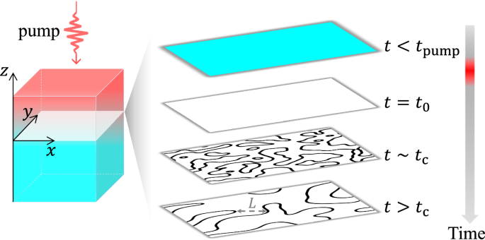
At t = t_pump, the surface region is pumped by an ultrafast pulse represented by the red segment on the time axis. An order parameter domain wall is created at t = t₀ on the white interface. The four planes on the right show the order parameter configuration of the interface at different times. The black curves denote the vortex strings.

Full size image

In this work, we propose that due to fluctuations, the domain wall will decay following a two-stage dynamics. In the first stage, the domain wall decays by the exponential growth of unstable fluctuations^17,32 of ψ on the wall, which happens both in the U(1) symmetric case, and in the system with a weak Z₂ term. The dynamics are characterized by increasing magnitude and correlation length of the fluctuations. At the end of the first stage, around a timescale t ≃ t_c, the wall is transformed into an interface containing randomly distributed topological defects, as shown by the vortex strings in Fig. 1 for a 3D system. In 2D systems, the interface is 1D and the defects are vortices and antivortices.

In the second stage, the motion and annihilation of topological defects on the interface dominate the dynamics. It happens under driving forces originating from the tension of the vortex strings in 3D systems and the attraction between vortices and antivortices in 2D systems^{33,34,35,36,37}. Universal features of the second-stage dynamics are characterized by a mean distance L(t) between the defects on the interface. The system undergoes a self-similar evolution with a global increase of L(t), leading to a coarsening phenomenon^32,33,34,36, as illustrated in Fig. 1. We show that in 3D systems, the coarsening dynamics exhibits a diffusive behavior in both the U(1)-symmetric case and the case with the additional weak Z₂ term, i.e., the length scale increases as L(t) ∝ t^1/2. In 2D systems with the weak Z₂ term, L(t) ∝ t^p exhibits a crossover from p ≈ 1/2 to p ≈ 0 as L gets larger, namely a diffusive-to-sub-diffusive crossover. The length scale L(t) can be measured from the structure factor in time-resolved X-ray diffraction experiments^38,39.

U(1)-symmetric model

We consider the “model A” dynamics^40,41, whose mean-field version is also called the ‘TDGL equation’, together with a U(1)-invariant free energy:

Here ψ(r, t) = ψ₁ + iψ₂ is the dimensionless complex order parameter, γ is the relaxation rate, E_c is the condensation energy density, D is the space dimension, α ~ (T − T_c)/T_c is negative at a temperature T below the critical temperature T_c, and ξ₀ is the bare coherence length. The thermal noise field η = η₁ + iη₂ arises from a thermal bath made of the other degrees of freedom, including high-energy electrons and phonons. We characterize the noise by a correlator (langle {eta }_{i}({boldsymbol{r}},t){eta }_{{i}^{{prime} }}({{boldsymbol{r}}}^{{prime} },{t}^{{prime} })rangle =2T{(gamma {E}_{{rm{c}}})}^{-1}{delta }_{i{i}^{{prime} }}delta ({boldsymbol{r}}-{{boldsymbol{r}}}^{{prime} })delta (t-{t}^{{prime} })) with an effective temperature T of the bath and (i/{i}^{{prime} }=1,2). Here the Ginzburg parameter (zeta =| alpha {| }^{D/2-2}T/({E}_{{rm{c}}}{xi }_{0}^{D})) plays the role of a dimensionless measure of the fluctuations in the non-equilibrium process as well as the equilibrium thermal fluctuations^17,42. Eqs. (1)(2) are reasonable approximations to the dynamics of the mean-field order parameter and its fluctuations at temperatures close to T_c^40,42 in incommensurate CDW^15,16, spin density waves (SDW)⁴³, excitonic insulators (EI), and Bardeen-Cooper-Schrieffer (BCS) superconductors^17,41,42,44. A microscopic derivation of the free energy model from an electron-phonon coupling Hamiltonian is presented in Supplementary Note 7, which shows ({E}_{{rm{c}}} sim nu {T}_{{rm{c}}}^{2}) with (nu sim {p}_{{rm{F}}}^{D}/{E}_{{rm{F}}}) being the density of states of electrons contributing to the Fermi surface nesting. Here p_F and E_F denote the Fermi momentum and Fermi energy of the metallic state without the CDW formation. Note that the CDW often has different coherence lengths in different directions while Eq. (2) is written in a rescaled spatial coordinate so that it appears isotropic. Around T_c, one has ξ₀ ~ v_F/T_c where v_F = E_F/p_F denotes the Fermi velocity^45,46. This leads to (zeta sim {T}_{{rm{c}}}^{D-1}/{E}_{{rm{F}}}^{D-1}| alpha {| }^{D/2-2})^17,42 which is similar to SDW, EI, and BCS superconductors^43,47,48,49.

We first consider the 2D domain wall in the 3D systems (D = 3), where the domain wall in Fig. 1 is set as the z = 0 plane. An order parameter configuration of the domain wall satisfies the saddle-point condition δF/δψ = 0. Without loss of generality, we choose the real solution ({psi }_{0}({boldsymbol{r}})=sqrt{| alpha | }tanh (z/xi )) as shown by the gray line in Fig. 2a, where (xi ={xi }_{0}/sqrt{| alpha | }) is the coherence length.

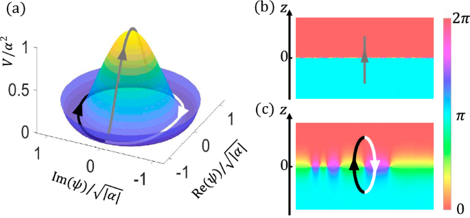
a The ‘Mexican hat’ free energy landscape (the potential part) of Eq. (2) plotted on the complex plane of ψ. b, c The phase of ψ plotted on the y– z plane at (b) t = t₀ and (c) t ≥ t_c, showing the domain wall at z = 0. The ψ and free energy along the gray, black, and white lines are also plotted in (a). In the initial domain-wall configuration, ψ = ψ₀(z) changes from (-sqrt{| alpha | }) to (sqrt{| alpha | }) crossing the potential peak along the gray line. To lower the energy, ψ fluctuates in the imaginary direction. After t_c, random phase domains appear on the interface. The loop denoted by black and white lines in (c) encloses a vortex with a phase winding 2π. In a 2D interface of a 3D system, the interface becomes full of vortex-strings as shown in Fig. 1.

Full size image

To study the first stage of dynamics, we set t₀ = 0 and write ψ(r, t) = ψ₀(r) + δψ(r, t) where δψ = ϕ₁ + iϕ₂ is the fluctuation field with the real part ϕ₁ and imaginary part ϕ₂. The linearized dynamics of δψ is expanded from Eq. (1) as

where a = 1, 2, ({hat{L}}_{1}=-{xi }_{0}^{2}{partial }_{z}^{2}+2alpha +6{psi }_{0}^{2}), ({hat{L}}_{2}=-{xi }_{0}^{2}{partial }_{z}^{2}+2alpha +2{psi }_{0}^{2}), and ({nabla }_{{boldsymbol{R}}}^{2}={partial }_{x}^{2}+{partial }_{y}^{2}) is the Laplacian in D − 1 dimensions. The eigen-function of ({hat{L}}_{a}-{xi }_{0}^{2}{nabla }_{{boldsymbol{R}}}^{2}) can be written as ({phi }_{a}^{{boldsymbol{K}}}({boldsymbol{r}})={u}_{a}(z){e}^{i{boldsymbol{K}}cdot {boldsymbol{R}}}) with eigenvalue ({epsilon }_{a}+{xi }_{0}^{2}{K}^{2}), where u_a(z) is the eigen-function of ({hat{L}}_{a}) with eigenvalue ϵ_a. Here R(K) denotes the spatial coordinate (momentum) in the (D − 1)-dimensional plane normal to z. Eigenvalues of ({hat{L}}_{1}) are all non-negative, while ({hat{L}}_{2}) has one negative eigenvalue, ϵ₂ = α, corresponding to a ‘bound-state’ eigen-function u₂(z) = sech(z/ξ), see the Supplementary Note 2. It implies that the long-wavelength fluctuations in the imaginary part direction, written as ({phi }_{2}^{{boldsymbol{K}}}({boldsymbol{r}})propto ,text{sech},(z/xi ){e}^{i{boldsymbol{K}}cdot {boldsymbol{R}}}) with (K ,<, sqrt{| alpha | }/{xi }_{0}), will grow exponentially in time with the exponent (left(| alpha | -{xi }_{0}^{2}{K}^{2}right)gamma t)¹⁷.

With ϕ₂(r) = φ(R, t)sech(z/ξ), the correlation function C(R, t) = 〈φ(0, t)φ(R, t)〉 depicts the real space structure of the fluctuation within the interface. From Eq. (3), it has the following analytical expression for γt ≫ 1/∣α∣ (see the Supplementary Note 2):

with the modified Bessel function I₀ of the first kind. Therefore, the fluctuation magnitude grows exponentially with the correlation length growing as (L(t)=4{xi }_{0}sqrt{gamma t}), a diffusive behavior. Note that due to the initial fluctuations (langle {phi }_{2}({boldsymbol{r}}){phi }_{2}({{boldsymbol{r}}}^{{prime} })rangle sim 1/| {boldsymbol{r}}-{{boldsymbol{r}}}^{{prime} }|) at long distances, the spatial correlation crosses over from an exponential decay at R ≪ L(t) to a power law decay (Cleft({boldsymbol{R}},tright)propto L(t)/R) at R ≫ L(t). The first-stage dynamics ends at a crossover time t_c when the fluctuation becomes so large that the linear approximation in Eq. (3) fails, and the ∣ψ∣⁴ term in Eq. (2) starts to stop its growth. One may estimate this timescale by 〈∣ψ(r, t_c)∣²〉 ~ ∣α∣, which gives C(0, t_c) ~ ∣α∣ and (gamma {t}_{{rm{c}}} sim {(2| alpha | )}^{-1}ln ({zeta }^{-1})). Note that γt_c thus obtained is much larger than 1/∣α∣ given that ζ is small enough.

At t ≃ t_c, the interface consists of randomly distributed positive-ϕ₂ and negative-ϕ₂ domains with the typical domain size of (4{xi }_{0}sqrt{gamma {t}_{{rm{c}}}})¹⁷. Boundaries between the domains quickly relax into stable topological defects with the phase winding ±2π, as illustrated in Fig. 2c, meaning that the interface becomes full of randomly distributed 2D vortex strings as in Fig. 1.

At t ≳ t_c, the second stage of dynamics takes over, which has been argued to be a coarsening dynamics³² of the vortex strings. Specifically, distributions of the vortex strings at different times show a statistical self-similarity, which is characterized by a growing correlation length L(t), or the typical inter-string distance. The coarsening dynamics with L(t) ∝ t^p and p > 1/2, p = 1/2, and p < 1/2 are referred to as superdiffusive, diffusive, and sub-diffusive dynamics, respectively. Eq. (1) implies the equation of motion for the length scale:

see refs. ^32,33,34,36 and the Supplementary Note 3. Here (lambda (L)frac{dL}{dt}) and F_d(L) are the frictional force with a friction coefficient λ(L) and the driving force acting on a unit length of the vortex string, respectively. Eq. (5) is nothing but a balance equation between the two forces. Consider a circular vortex-string loop with the diameter L, a typical topological defect, its energy is (E sim | alpha | {E}_{{rm{c}}}{xi }_{0}^{2}Lln (L/xi ))³². Therefore, the driving force that contracts the loop is ({F}_{{rm{d}}}(L) sim {L}^{-1}dE/dL sim | alpha | {E}_{{rm{c}}}{xi }_{0}^{2}{L}^{-1}ln (L/xi )) in the large L limit. The friction coefficient (lambda (L) sim {gamma }^{-1}{E}_{{rm{c}}}| alpha | ln (L/xi )) is derived from the damping term³², i.e., first-order time derivative term in Eq. (1). Combining these two, we obtain a solution of Eq. (5) in the large-L limit as (L(t) sim {xi }_{0}sqrt{gamma t}), which manifests a diffusive coarsening dynamics.

We numerically simulated Eq. (1) with the domain-wall initial condition and observed the coarsening dynamics. To evaluate the length scale L(t) in the simulation, we count a number N of vortices in the y–z planes for each discrete x, average N over each x in ten independent simulations, and define L = L_y/〈N〉, where L_y is the system size along y. Figure 3a shows L versus time by a log-log plot in the interval of ({log }_{10}(L/xi )in (1,1.2)), from which we estimate the exponent p by a linear fit ({log }_{10}left(L/xi right)=p{log }_{10}(| alpha | gamma t)+{c}_{0}). The estimate gives p = 0.45 for the 2D interface of a 3D system. The discrepancy from the theoretical result may be because the simulation has not entered the long-time region.

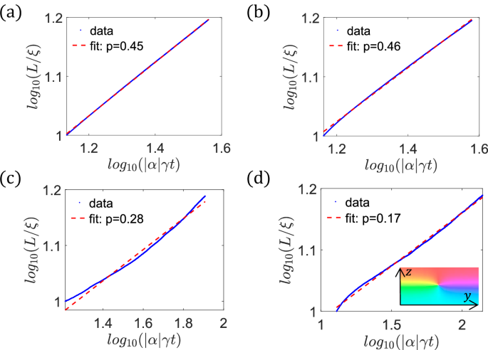
In the numerical simulation, space and time are discretized by step sizes 0.5ξ and 0.03(∣α∣γ)⁻¹. Data points are selected within ({log }_{10}(L/xi )in (1,1.2)). The results are statistical averages over ten independent simulations. a The 3D U(1) symmetric case. b The 3D U(1) breaking case with β/∣α∣ = 0.1. Both (a) and (b) are simulated in a L_x × L_y × L_z grid with L_z/ξ = 60, L_x/ξ = L_y/ξ = 1280. c, d The 2D case with the Z₂ term β/∣α∣ being (c) 0.001 and (d) 0.1. The phase distribution of a topological defect is sketched in the inset of (d) with the same colorbar as Fig. 2b, c. Both (c) and (d) are simulated in a L_y × L_z grid with L_z/ξ = 120, L_y/ξ = 38,400.

Full size image

Effects of a Z
₂ term

To model the case without the U(1) symmetry, we add a term (2beta {psi }_{2}^{2}) (‘Z₂ term’) with β > 0 to the free energy density in Eq. (2), reducing the U(1) symmetry to a Z₂ ⊗ Z₂ symmetry under the transformation ψ₁₍₂₎ → ± ψ₁₍₂₎. Due to the Z₂ term, the low-temperature equilibrium state is long-range ordered even for a 2D system so that a well-defined 1D domain wall could be generated. This model describes commensurate CDW/SDW^46,50 and certain excitonic insulators¹⁹, etc. As shown below, the decay process of the domain wall for the small β case is characterized by a similar two-stage dynamics as the U(1) symmetric case, while the scaling behavior may be different.

For the first-stage dynamics, the Z₂ term modifies ({hat{L}}_{2}) in Eq. (3), ({hat{L}}_{2}=-{xi }_{0}^{2}{partial }_{z}^{2}+2(alpha +beta )+2{psi }_{0}^{2}), so that the lowest eigenvalue of ({hat{L}}_{2}) becomes α + 2β. For β > ∣α∣/2, the eigenvalue is positive, and the domain wall is stable against any fluctuation of the imaginary part of ψ. For β < ∣α∣/2, the mode ({phi }_{2}^{{boldsymbol{K}}}({boldsymbol{r}}) propto ,text{sech},(z/xi ){e}^{i{boldsymbol{K}}cdot {boldsymbol{R}}}) with (K ,<, sqrt{| alpha | -2beta }/{xi }_{0}) grows exponentially in time. The growth is characterized by the correlation function C(R, t). The correlation function in the long-time regime with γt ≫ 1/β and γt ≫ 1/(∣α∣ − 2β) is computed from Eq. (3) as

where ({c}_{1}approx sqrt{| alpha | /beta }) if β ≪ ∣α∣. Similar to Eq. (4), one has a growing correlation length (L(t) sim {xi }_{0}sqrt{8gamma t}). The crossover time to the second-stage dynamics is (gamma {t}_{{rm{c}}} sim {(2| alpha | )}^{-1}ln ({zeta }^{-1})) for β ≪ ∣α∣, given that (ln ({zeta }^{-1})gg | alpha | /beta) such that t_c is in the long-time regime. Note that although the domain wall is locally stable for β > ∣α∣/2 in our calculation, it will finally decay in pump-probe experiments from other effects such as the nonzero curvature of the domain wall due to the finite spot size of lasers, see the Supplementary Note 8. It may also tunnel into another type of domain wall by nucleation processes, which we leave for future study.

The coarsening dynamics of the topological defects with the Z₂ term are also described by the balance equation Eq. (5), while the friction coefficient λ(L) and the driving force F_d(L) depends on a spatial profile of the topological defect that is deformed by the Z₂ term. In the case of β ≪ ∣α∣, the free energy density f is dominated by its phase part,

Even with the small β, the topological defect is no longer a perfectly circular vortex, but connects two different sine-Gordon solitons ({theta }_{0}^{pm }=,text{arg},left(sinh (sqrt{2beta }z/{xi }_{0})pm iright))⁵¹, which is sketched in the inset of Fig. 3d. When the distance r from the vortex core in the 2D plane is much smaller than a length scale ({xi }_{0}/sqrt{2beta }), the spatial profile approaches the form of a circular symmetric vortex. For ({r},gg, {xi }_{0}/sqrt{2beta }), the profile approaches the sine-Gordon solitons as (theta approx {theta }_{0}^{pm }+s({boldsymbol{r}})), where (s({boldsymbol{r}}) sim {e}^{-rsqrt{2beta }/{xi }_{0}}) decays exponentially.

As a result, the coarsening dynamics crosses over between two asymptotic time domains. In the early-time domain with (L(t),ll, {xi }_{0}/sqrt{2beta }), adjacent defects see each other as circular symmetric vortices. Therefore, the driving force and frictional force are the same as the U(1) symmetric case. In 2D systems, they are ({F}_{{rm{d}}}(L) sim {E}_{{rm{c}}}| alpha | {xi }_{0}^{2}/L), and (lambda (L) sim {E}_{{rm{c}}}| alpha | ln (L/xi )/gamma), respectively. From Eq. (5), one has (L(t) sim {xi }_{0}sqrt{gamma t/ln (| alpha | gamma t)}), which is nearly diffusive in the large-γt limit. In 3D systems, the calculation is explained below Eq. (5). In the late-time domain with (L(t),gg, {xi }_{0}/sqrt{2beta }), the adjacent vortices see each other as the sine-Gordon solitons. Thereby, the friction coefficient becomes a constant λ ~ E_c∣α∣/γ. The driving force in the 2D system becomes short-range attraction between vortices and antivortices with ({F}_{{rm{d}}}(L) sim {xi }_{0}{E}_{{rm{c}}}| alpha | sqrt{2beta }{e}^{-Lsqrt{2beta }/{xi }_{0}}), while the driving force in the 3D system is dominated by the string tension with ({F}_{{rm{d}}}(L) sim {xi }_{0}^{2}{E}_{{rm{c}}}| alpha | {L}^{-1}), see the Supplementary Note 3. This results in the following scaling for the late-time domain of the coarsening dynamics,

Thus, the coarsening dynamics in the 2D systems exhibit a diffusive-to-sub-diffusive crossover as L goes from ({L},ll, {xi }_{0}/sqrt{2beta }) to ({L},gg, {xi }_{0}/sqrt{2beta }), while that in the 3D systems are always diffusive.

Numerical simulations of Eq. (1) with the Z₂ term shows consistent coarsening dynamics. In Fig. 3b, c, d, we fit the value of p in the interval of ({log }_{10}(L/xi )in (1,1.2)) for several β/∣α∣. We get p = 0.46 in the 3D systems with β/∣α∣ = 0.1 (Fig. 3b), which is consistent with the diffusive dynamics. In the 2D systems, we obtain p = 0.28 and 0.17 with β/∣α∣ = 0.001 (({L},<, {xi }_{0}/sqrt{2beta })) and 0.1 (({L},>, {xi }_{0}/sqrt{2beta })), respectively (Fig. 3c, d), which is consistent with the diffusive-to-sub-diffusive crossover.

Stability of the interface

In addition to the motion within the interface, the defects also move in the z-direction due to the thermal noise η. From Eq. (1), the z-direction motion of a defect is a Brownian motion given by d(z/ξ₀)/d(γt) = H_z with a random force H_z dependent on the defect size. For a typical defect with size L, the random force for a vortex satisfies

Here ({h}_{z}(L)=int,{d}^{2}{boldsymbol{r}},{({partial }_{z}theta )}^{2}) where θ(r) is the profile of a vortex with size L discussed below Eq. (7), see the Supplementary Note 3. For the U(1) symmetric case as well as for the ({L},ll, {xi }_{0}/sqrt{2beta }) case with a nonzero β, one has ({h}_{z}(L) sim ln (L/xi )), while it is hard to evaluate h_z(L) for the other cases. Eq. (9) implies that as long as ζ is small, the z-direction motion of the defects is negligible and the interface is stable.

Effects of the inertia term

So far, we have clarified the decaying process of the domain wall in terms of the “model A” dynamics, Eq. (1). The “model A” dynamics neglects the inertia of the order parameter, the ({partial }_{t}^{2}psi) term, while the inertia is crucial for the inversion of the order parameter by the pump pulse that generates the domain wall^27,28,29,30. Thus, we now proceed to add the inertia term ({gamma }_{0}^{-2}{partial }_{t}^{2}psi) to the left-hand side of Eq. (1), and discuss how the decaying processes of the domain wall are modified. Note that microscopic derivations of the relevant TDGL theory^42,52 gives γ, γ₀ ~ T for pure electronic density-wave orders arising from Fermi surface nesting, see ref. ⁴² and Appendix E of ref. ⁵², while mixing with lattice distortions and electron-phonon scattering may significantly modify these parameters.

In the first-stage dynamics, a small ∣α∣ suppresses the inertia term more effectively than the damping term. Thus, as long as the temperature is close to T_c where ∣α∣ ≪ 1, the inertia term does not change the qualitative picture of the first-stage dynamics, modifying only the coefficients. Specifically, the time-dependent correlation length in Eqs. (4),(6) is renormalized by a factor (1/sqrt{kappa }) with (kappa =sqrt{1+4(| alpha | -2beta ){gamma }^{2}/{gamma }_{0}^{2}}), see the Supplementary Note 4.

In the second-stage dynamics, the ({partial }_{t}^{2}psi) term gives the topological defect an inertial mass (m(L)=lambda (L)gamma /{gamma }_{0}^{2})⁵³, which is dependent on the defect size L. Thereby, Eq. (5) is modified into

see the Supplementary Note 4. Note that all the results of L(t) satisfying Eq. (5) obtained in this work satisfy Eq. (10) in the long-time limit, when the term m(L)d²L/dt² is much smaller than the other two terms.

Estimation of parameters and timescales

Phenomenological parameters γ, ξ₀, ζ, and α determine the timescale of the dynamics. In relevant CDW materials such as RTe₃ (R = La, Sm, Tb, Ce), 1T-TaS₂, and 1T-TiSe₂^54,55,56, the relaxation time is roughly 1/γ ~ 1 ps from ultrafast experiments^{11,16,20,27,29,57}. From the expression ξ₀ ~ v_F/T_c, ξ₀ is estimated as several nanometers for LaTe₃²², while a similar value was obtained for 1T-TaS₂ from the domain-wall width in scanning tunneling microscopy images²⁰. Experiments are typically performed in 3D materials, where ({T}_{{rm{c}}}^{D-1}/{E}_{{rm{F}}}^{D-1} sim 1{0}^{-4}) given that E_F ~ 10⁴− 10⁵ K for metals and T_c ~ 10²– 10³ K. Therefore, the Ginzburg parameter is estimated by (zeta sim 1{0}^{-4}/sqrt{| alpha | }) for a certain experimental temperature. For example, in room-temperature (T ≈ 300 K) experiments for SmTe₃ with T_c = 416 K or LaTe₃ with T_c = 670 K^11,29, one has (sqrt{| alpha | } sim 1) and ζ ~ 10⁻⁴. The first-stage dynamics finishes at a crossover time t_c ~ 10γ⁻¹ ∼ 10 ps. The second-stage dynamics will continue until L(t) reaches a certain length scale L_s when the domain wall starts to interact with other domain walls or the sample surface. L_s is the domain-wall depth or the inter-domain-wall distance if multiple domain walls are generated. From the literature^28,29, an estimation gives L_s/ξ₀ ~ 10 in 3D systems. Therefore, the scaling (L(t) sim {xi }_{0}sqrt{gamma t}) gives a timescale ~10² ps for the second-stage dynamics.

Experimental scheme

The CDW order induces a lattice distortion b (r) ∝ ψ(r, t)e^iQ⋅r, where Q is the CDW wavevector lying in the x– y plane, see the Supplementary Note 7. One could measure the evolution of the CDW order from the lattice structure factor in ultrafast x-ray scattering^38,39,58. For example, in a recent ultrafast x-ray scattering experiment for LaTe₃ which exhibits an incommensurate CDW, the material was excited by a 1.55 eV, 35 fs optical pump pulse with the fluence of 8 mJ/cm² and probed by a 50 fs, 10 keV hard x-ray pulse³⁸. To investigate the dynamics of the z = 0 interface parametrized by R, one could extract a structure factor defined by S(R, t) ≡ 〈b^†(0, t)b(R, t)〉 ∝ 〈ψ^†(0, t)ψ(R, t)〉e^iQ⋅R, whose Fourier transform (tilde{S}({boldsymbol{K}},t)) has a peak at K = Q with the peak intensity corresponding to the amplitude ∣ψ∣² and the inverse of the full width at half maximum (IFWHM) corresponding to the correlation length L(t). In the long-time regime of the first-stage dynamics, Eqs. (4)(6) predict the peak intensity to show an exponential growth and the IFWHM to exhibit a diffusive growth. In the second-stage dynamics, the IFWHM is expected to show a diffusive growth for 3D materials while the peak intensity has no significant growth since the growth of fluctuation magnitude has saturated.

Our theory enriches the mechanism of topological defect generation in ultrafast experiments^{11,25,59,60,61,62}. It applies to a wide class of systems with order parameters breaking a (quasi) continuous symmetry, such as charge order^{23,46,57,63,64}, spin order⁴³, excitonic order^19,48,49, and superconductivity^17,41,42,44.

In some experiments for 3D systems, a strong pump fluence could generate multiple domain walls at different depths in the z direction with a typical inter-wall distance L_z^27,28,29. In this paper, we focused on the decaying dynamics of an individual domain wall neglecting the interaction between the walls. This is appropriate as long as the inter-wall distance L_z is much larger than the typical size L of the topological defects on the walls, such that each wall evolves independently with a diffusive growth of in-plane correlation length L while L_z does not grow. In other words, the measured correlation-length dynamics depend on the direction of the measurement. This might be relevant to a recent pump-probe experiment that reports anomalous sub-diffusive coarsening dynamics of the CDW in LaTe₃³⁸.

Optically generated domain walls may also appear and lead to interesting dynamics in other situations that warrant further investigation^65,66,67, e.g., the domain wall between superconducting orders with different chirality⁶⁸. Another example is the system with competing orders¹⁷: a real field ψ breaking a Z₂ symmetry (e.g., commensurate CDW) competes with a complex field Ψ = Ψ₁ + iΨ₂ breaking a U(1) symmetry (e.g., superconductivity or incommensurate CDW)^63,64 such that ψ dominates and Ψ is completely suppressed in equilibrium. If a pump pulse generates a domain wall of ψ, the fluctuations of Ψ may become unstable on the domain wall and grow into a random domain structure with increasing correlation length. A preliminary study of a model with a quartic competing term ∣Ψ∣²ψ² is provided in Supplementary Note 5, while it is meaningful to perform a systematical study with various competing terms between multi-component orders.

Both analytical and numerical results in this work are obtained by the “model A” dynamics, Eq. (1). The results of the first-stage dynamics are derived from the linearized dynamical equation, Eq. (3). The analytical results of the second-stage dynamics are obtained from the force-balance equation, Eq. (5), which is derived from Eq. (1). In the numerical simulations, the “model A” dynamical equation was rescaled by

with (b=sqrt{| alpha | }) and (bar{alpha }=-1). We further define τ = ∣α∣γt, (tilde{{boldsymbol{r}}}={boldsymbol{r}}/xi) and (tilde{nabla }=partial /partial tilde{{boldsymbol{r}}}) and update (bar{psi }) after each time step according to the dynamical equation given in the following form:

The rescaled noise correaltor reads (langle {bar{eta }}_{i}(tilde{{boldsymbol{r}}},tau ){bar{eta }}_{{i}^{{prime} }}({tilde{{boldsymbol{r}}}}^{{prime} },{tau }^{{prime} })rangle =2zeta {delta }_{i{i}^{{prime} }}delta (tilde{{boldsymbol{r}}}-{tilde{{boldsymbol{r}}}}^{{prime} })delta (tau -{tau }^{{prime} })). (bar{eta }(tilde{{boldsymbol{r}}},tau )dtau) are generated by (scriptstyle{bar{eta }}_{i}(tilde{{boldsymbol{r}}},tau )dtau =sqrt{frac{2zeta dtau }{{Pi }_{j}d{r}_{j}}}{n}_{i}(tilde{r},tau )) with ({n}_{i}(tilde{r},tau )) being generated from independent standard normal distribution for each discretized (tilde{{boldsymbol{r}}}) and τ. The values of 2ζ and the discretization step sizes, dr_j=x,y,z and dτ, are provided in the caption of Fig. 3. The second-order derivative, ({tilde{nabla }}^{2}bar{psi }), is computed using the central difference method. A free boundary condition is applied along the z-direction, while periodic boundary conditions are imposed along the x– and y-directions.