Spin density wave in the bilayered nickelate La3Ni2O7−δ at ambient pressure
Introduction
The recent discovery of novel superconductivity with Tc up to 80 K in highly pressurized La3Ni2O7−δ has sparked extensive experimental and theoretical investigations1,2,3,4,5,6,7,8,9,10. While current theoretical studies primarily focus on the pairing mechanisms of its high-pressure phase11,12,13,14,15,16,17,18,19,20,21,22,23,24,25, understanding the magnetic ground state of La3Ni2O7−δ at low pressure is essential to elucidate the correlation between magnetism and the high-Tc superconductivity. For La3Ni2O7−δ at ambient pressure, resistivity measurements have suggested a possible spin density wave (SDW) phase below a transition temperature TSDW ~150 K26. However, early nuclear magnetic resonance (NMR) experiments mainly find evidence for charge ordering in La3Ni2O7−δ, although the existence of SDW is not completely ruled out27. More recently, resonant inelastic x-ray scattering (RIXS) experiments measuring the magnetic excitations of La3Ni2O7−δ single crystals clearly indicate the presence of in-plane magnetic correlations with Q = (0.25, 0.25) below 150 K, suggesting possible spin orders with double spin stripe (DSS) or spin-charge stripe (SCS) configurations28,29. The presence of the DSS order is also weakly evidenced by more recent NMR data29 and inelastic neutron scattering data30. Conversely, the SCS is favored as the SDW phase, qualitatively consistent with a field distribution with both high and low strengths observed in a positive muon spin relaxation (μ+ SR) study of polycrystalline La3Ni2O7−δ31.
Theoretical studies on the magnetic properties of La3Ni2O7 have primarily focused on determining the magnetic ground state by comparing energies of various magnetic configurations from density functional theory (DFT) calculations32,33,34. Yi et al.32 identified the A-type antiferromagnetic (AFM) configuration as the magnetic ground state. Chen et al.35, based on experimental RIXS spectra, reproduced the observed magnon dispersion using a simplified J1–J2–J3 Heisenberg model. However, current theoretical studies on the magnetism of La3Ni2O7 cannot fully explain the experimental observations. Notably, oxygen vacancies are commonly present in experimental samples of La3Ni2O7. While the impact of oxygen vacancies on the electronic structure and superconductivity has been investigated based on DFT calculations32,36,37, their effect on the magnetism of La3Ni2O7 remains elusive.
In this work, we investigate the magnetic properties of La3Ni2O7−δ at ambient pressure using DFT calculations. For δ = 0, our results indicate that the DSS phase, characterized by a (0.25, 0.25) in-plane modulation vector, is the favored magnetic ground state. The presence of oxygen vacancies leads to the vanishing of Ni magnetic moments nearest to the vacancy sites, effectively creating charge sites. For moderate δ values, our theoretical SDW phase exhibits features of both DSS and SCS configurations, reconciling the seemingly contradictory experimental findings that suggest both DSS and SCS as candidates for the SDW phase. At higher oxygen vacancy concentrations, such as δ = 0.5, we predict a short-range ordered ground state with spin-glass-like magnetic structures, disrupting the (0.25, 0.25) modulation vector. Oxygen vacancies also reduce the TSDW due to the dilution of dominant exchange interactions. Notably, the magnetic ordering naturally brings concurrent charge ordering and orbital ordering, due to the symmetry lowering faciliated by spin-lattice coupling. Furthermore, our findings indicate that a random distribution of oxygen vacancies may need to be considered to achieve spin wave spectra consistent with experimental data. We also offer a plausible explanation for experimental observations, such as the insensitivity of the measured TSDW to different samples and the lack of direct evidence for long-range magnetic ordering.
Results
Crystal structure
At ambient pressure, bulk La3Ni2O7 crystallizes in an orthorhombic structure with the space group Amam and lattice parameters a = 5.393 Å, b = 5.448 Å, and c = 20.518 Å1. As illustrated in Fig. 1a, each unit cell of La3Ni2O7 comprises two Ni-O bilayers, with each Ni atom coordinated by six O atoms, forming NiO6 octahedra. The oxygen atoms occupy four inequivalent sites: two within each Ni-O layer, and the other two at the inner-apical and outer-apical positions, respectively.
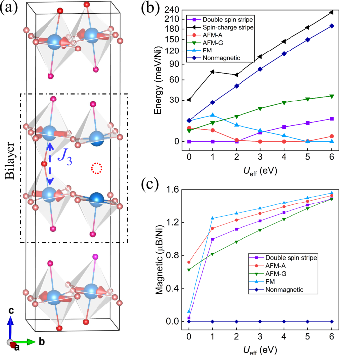
a The crystal structure of La3Ni2O7−δ. The Ni atoms, outer-apical oxygen, inner-apical oxygen, and in-plane oxygen are represented by blue, rosy, red, and pink spheres, respectively. The red arrows denote spins. The dashed red circle indicates an inner-apical oxygen vacancy. The calculated (b) total energies and (c) average magnetic moments with different Ueff in La3Ni2O7.
Magnetic order
Magnetic properties from DFT + U calculations are typically sensitive to the U values. Therefore, we first perform total energy calculations for several representative magnetic configurations across a range of U values using the DFT+ U method38. We consider the ferromagnetic (FM), A-type AFM (AFM-A), G-type AFM (AFM-G), DSS, and SCS configurations as illustrated in Fig. 2a, b, d. The DSS corresponds to an up-up-down-down stripe arrangement along each in-plane lattice vector in the tetragonal lattice setting, while the SCS can then be constructed by alternately replacing half of the local spins in the DSS by spinless charge sites. To be consistent with experimental literatures28,29,30, we adopt the DSS and SCS to describe these two spin configurations throughout our paper. Our calculated energies indicate that the DSS configuration has the lowest energy among the selected configurations when Ueff is no larger than 2 eV (see Fig. 1b), consistent with experimental findings29,30. In the Ueff range of 3 to 4 eV, the AFM-A configuration emerges as the magnetic ground state. Conversely, for Ueff values exceeding 5 eV, the ground state transitions to FM. The only distinction between the AFM-A and FM configurations lies in the interlayer magnetic correlations, suggesting a shift from AFM to FM interlayer interactions with increasing Ueff (see Fig. 1b). Although the SCS has been proposed to fit the experimental magnetic excitation spectra well, its calculated energy consistently exceeds that of the DSS across all Ueff values, favoring the DSS as the SDW phase. The results from our DFT + U calculations are further supported by our HSE06 calculations (see Supplementary Note 3 Table SII). Moreover, the calculated magnetic moments increase with larger Ueff values due to the increased localization of Ni 3d electrons. Given that experimental measurements report relatively weak magnetic moments, with average values of 0.08 μB/Ni29 and 0.55 μB/Ni39, we primarily present results with Ueff = 1 eV unless stated otherwise. Although larger U values (U ~ 2–4 eV) are usually employed to study electronic structures of La3Ni2O711,40, especially for the case under high pressure, our calculations indicate that a smaller U value may be more suitable for the description of its magnetic properties, which is also consistent with the findings of two recent theoretical studies on the SDW of La3Ni2O741,42. It is worth noting that, although all Ni atoms occupy symmetrically equivalent sites in the space group Amam, the symmetry lowering induced by the DSS phase causes the calculated magnetic moments to split into two groups, with amplitudes of 1.2 μB and 0.7 μB, respectively(see Supplementary Note 1 Table SI and Fig. 4). This significant splitting of magnetic moments implies qualitative splitting of electron occupations on Ni sites, which may introduce a component of charge order. Indeed, our further calculations indicate that the DSS phase already consists of formally Ni2+ (1.2 μB) and Ni3+ (0.7 μB), which we will discuss in details in subsequent sections. In spite of this, to be consistent with literatures and avoid ambiguity, we keep denoting this phase as DSS throughout this work.
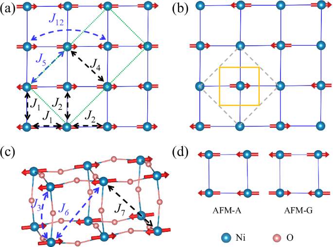
a The DSS configuration, with the exchange paths represented by dashed lines with double arrows. The green box represents a magnetic unit cell in the DSS configuration. Red arrows represent spin up and down. b The SCS configuration. The yellow box and the dashed box denote a unit cell in real space and the corresponding first Brillouin zone, respectively. c Exchange paths for J‘s are represented by dashed lines with arrows, where black color indicates ferromagnetic interactions and blue color indicates antiferromagnetic interactions. Ni and O atoms are illustrated as blue and pink spheres, respectively. d Schematic representation of different magnetic configurations.
To further explore the magnetic properties, we employ the classical Heisenberg model to describe the magnetic interactions in La3Ni2O7, represented by the Hamiltonian,
where Jij are the Heisenberg exchange interactions between Ni spins Si and Sj. To adequately capture the relevant magnetic interactions, we consider exchange interactions with Ni-Ni bond lengths up to 8 Å. In total, there are 12 inequivalent types of J’s, among which J1, J2, J4, J5, and J12 are interactions within each Ni-O layer, while J3 and J6 – J9 are interlayer interactions. J10 and J11 represent interactions between bilayers. The major exchange interactions are illustrated in Fig. 2a, c, with calculated results presented in Table 1. Within each Ni-O layer, the FM interactions J1 and J4, and the AFM interactions J5 and J12, favor the formation of an in-plane magnetic structure with a wavevector of (0.25, 0.25). The FM interaction J2 impedes the formation of this magnetic phase, introducing magnetic frustration. However, this frustration is relatively weak, thus allowing the (0.25, 0.25) magnetic phase to persist. On the other hand, the interlayer interactions are predominantly governed by the strong AFM interaction J3, which is an order of magnitude larger than the other J’s. It is worth noting that the DSS and SCS only refer to in-plane spin arrangement, which is not directly affected by the strong J3. However, in practice, antiferromagnetic interlayer coupling is implied in the DSS and SCS35. In this sense, the interlayer coupling affects the formation of the DSS and SCS, by enforcing an AFM arrangement between the Ni atom layers within each bilayer. In contrast, the inter-bilayer interactions J10 and J11 are negligibly small. These results are consistent with the exchange interactions extracted from experimental RIXS data35.
Based on the calculated J’s values, we explore the magnetic phase diagrams using a replica-exchange Monte Carlo (MC) method43,44. Our MC simulations confirm the DSS as the ground state, consistent with our total energy calculations. However, the simulated TSDW is ~232 K, which is significantly higher than the experimental values26,27,28,29. This discrepancy could be attributed to limitations in our DFT + U calculations, which may not accurately capture all relevant magnetic interactions. Additionally, we find that oxygen vacancies may also play an important role in the magnetic properties, which we will discuss further in the subsequent sections.
Oxygen vacancy
We conduct first-principles calculations to investigate the oxygen vacancy configurations for three types of oxygen positions: inner-apical oxygen, in-plane oxygen, and outer-apical oxygen (see Fig. 1a). Our calculations reveal that the inner-apical oxygen vacancy is the most stable, with significantly lower formation energies compared to the other two types of vacancies. This finding suggests that the inner-apical oxygen vacancies are more likely to form during practical material synthesis, consistent with experimental observations reported in ref. 45. Therefore, we only consider the inner-apical oxygen vacancies, implemented by removing the corresponding number of inner-apical oxygen atoms in a La3Ni2O7 supercell (see Supplementary Note 4). In experimental samples, the δ values are found to typically range from 0 to 0.529,31,39,45,46. To reduce computational cost from the supercell approach, we mainly perform DFT calculations with δ = 0.25 and δ = 0.5 using a 48-atom supercell. We then investigate the effect of vacancy concentrations on the magnetism and find that the magnetic moments of the Ni atoms nearest to the oxygen vacancies diminish to nearly zero ( ~0.03 μB), effectively forming charge sites. As shown in Fig. 1a, two charge sites can be produced by removing one oxygen atom. As a result, the presence of charge sites leads to a noticeable reduction in the average magnetic moment, which may contribute to the experimentally observed small magnetic moments of Ni29,31,39.
We then recompute the exchange interactions of La3Ni2O7−δ for δ = 0.25 and δ = 0.5, under which the original 12 J’s split into 48 J’s and 16 J’s, respectively (see Tables SIII and SV in Supplementary Note 4). Unsurprisingly, with oxygen vacancies, the J’s involving the introduced charge sites are among the most affected, with portions of J3, J4, J5, and J12 that connect at least one charge site, vanishing. For δ = 0.25, the J1 and the remainder of J5 and J12 largely retain their original AFM characteristics, albeit with reduced strength. The J4 changes from FM to AFM, while J2 remains FM. Consequently, the magnetic frustration is enhanced. The magnetic ground state with δ = 0.25 is expected to deviate from the DSS, with a lowered TSDW due to the dilution of the leading exchange interactions. Notably, the dominant J3 is found to be sensitive to the corresponding Ni-O-Ni bond lengths and angles. The magnitude of J3 increases with larger bond angles, supporting that J3 are superexchange interactions facilitated by the inner-apical oxygen atoms through the Ni(({d}_{{z}^{2}}))-O(pz)-Ni(({d}_{{z}^{2}})) pathways (see Tables SIV in the Supplementary Note 4). The ({d}_{{z}^{2}}) orbitals are expected to form a singlet state, leading to the strong antiferromagnetic J3.
When δ reaches 0.5, half of the Ni spins are converted into charges. With an ordered vacancy distribution as shown in Supplementary Note 4 Fig. S4c, the resulting magnetic configuration effectively becomes an ideal SCS, as shown in Fig. 2b. Consequently, all the nearest neighbor (NN) intralayer J’s (J1 and J2) are significantly weakened, as each J connects one spin and one charge (see Supplementary Note 4 Tables SIV). This scenario naturally reproduces the theoretical model proposed in ref. 28, where for the DSS phase, all the NN intralayer interactions are artificially set to zero to obtain magnetic excitations consistent with experimental data. With δ = 0.5, the corresponding TSDW is expected to be further lowered due to the increased presence of charges.
To confirm the impact of oxygen vacancies on the magnetic phase diagrams, we first perform MC simulations for both δ = 0.25 and δ = 0.5, using the J’s from direct DFT calculations with the ordered vacancy distributions (see Supplementary Note 4 Tables SIII and SV). Consistent with our qualitative analysis, we find that for δ = 0.25, the magnetic ground state becomes noncollinear and slightly deviates from the DSS phase (see Supplementary Note 5 Fig. S6b). Fourier analysis shows that the Q vector (0.25, 0.25) is preserved, but the TSDW decreases to 155 K. For δ = 0.5, the simulated magnetic ground state indeed effectively becomes an ordered SCS, but with noncollinear spins and a drastically reduced TSDW of 48 K (see Supplementary Note 5 Fig. S7). For δ > 0, the dilution of the strong interlayer interaction J3 raises the transition temperature of magnetic ordering.
However, oxygen vacancies are expected to be disordered in experimental samples. Therefore, to simulate a more realistic scenario, we also perform MC simulations with randomly distributed oxygen vacancies. In this case, approximations are made to simplify the calculations, with the J’s directly involving the charge sites set to zero and the other J’s assigned values from Table 1. The obtained phase diagram and magnetic structures are shown in Fig. 3 and Supplementary Note 6 Fig. S8. As expected, the simulated TSDW decreases with increasing δ. For 0 < δ < 0.5, the resulting magnetic ground state can be considered a mixture of the DSS and the SCS, characterized by a dominant global modulation vector (0.25, 0.25) (see Supplementary Note 6 Fig. S8), which is distinct from 214 nickelates, where the global wave vector continuously varies with doping47,48. A sudden drop in TSDW at δ ~ 0.3 marks the separation of two distinct phases. For 0 < δ < 0.3, the magnetic ground state is dominated by the DSS with collinear spin structures (red area in Fig. 3), while for larger δ (0.3 ≤δ < 0.5), the SCS outweighs the DSS, and the spin structures become slightly noncollinear (green area in Fig. 3). For δ ≥ 0.5, the calculated specific heat from the MC simulations shows a bump instead of a diverging peak, suggesting the presence of only short-range order. The corresponding spin structures become strongly noncollinear with spin-glass-like characteristics (blue area in Fig. 3). Our simulated phase diagram provides a natural explanation to reconcile the seemingly contradictory experimental findings that both the DSS and the SCS are proposed as candidates for the SDW phase. Nevertheless, our calculations indicate that oxygen vacancies notably affect the magnetic properties of La3Ni2O7, lowering TSDW and altering the ground state magnetic structures.
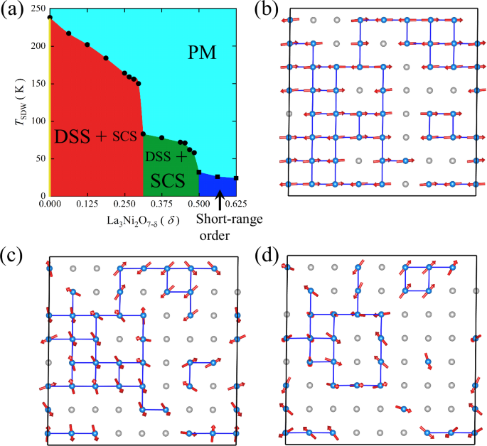
a Phase diagram of La3Ni2O7−δ obtained from MC simulations, where PM stands for paramagnetic. b–d Sketches of typical magnetic ground states from MC simulations with δ of 0.25, 0.375, and 0.5, respectively. Red arrows represent spin up and down.
Charge order and orbital order
Magnetic ordering with notable spiltting of magnetic momoments may naturally lead to concomitant charge ordering and orbital ordering. In the DSS phase, the emergence of the splitted magnetic moments of 1.2 μB (Ni1) and 0.7 μB (Ni2) can be attributed to the formation of different valence states of Ni ions. For δ > 0, the presence of inner-apical oxygen vacancies introduces non-magnetic Ni ions (Ni3) in addition to Ni1 and Ni2. Our calculated partial density of states (PDOS) of Ni1 and Ni2 with δ = 0.25 are very close to those with δ = 0 (see Supplementary Note 7 for the PDOS with δ = 0 and Fig. 4a for δ = 0.25), which suggests that the presence of moderate oxygen vacancies only has mild impact on the electronic configurations of Ni1 and Ni2. Therefore, for simplicity, we mainly discuss the PDOS with δ = 0.25, in which case, Ni1, Ni2 and Ni3 are all present.
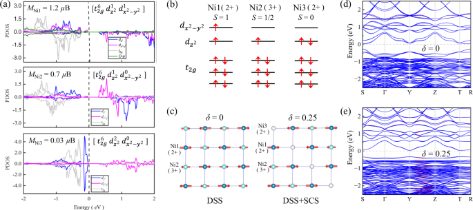
a Calculated partial DOS of Ni1, Ni2 and Ni3 for δ = 0.25. b Sketches of electron configurations of Ni1, Ni2 and Ni3. c Illustration of the calculated DSS phase with δ = 0, showing the alternating magnetic moments of Ni1 and Ni2 and the concomitant charge order. d Illustration of a calculated double spin/charge stripe phase with δ = 0.25, showing the concomitant charge order with Ni1, Ni2 and Ni3. Red arrows represent spins. Calculated electron band structures of (d) DSS phase with δ = 0 and (e) double spin/charge stripe phase with δ = 0.25. The red and blue lines represent spin-up and spin-down states, respectively.
Our DFT calculated PDOS indicates that the Ni1 has a valence state of 2+ with an electron configuration of (({t}_{2g}^{6},{d}_{{z}^{2}}^{1},{d}_{{x}^{2}-{y}^{2}}^{1})), while the Ni2 has an electron configuration of (({t}_{2g}^{6},{d}_{{z}^{2}}^{1})), corresponding to Ni3+(see Fig. 4a, b. In the perfect DSS phase with δ = 0, the orbital ordering originates from the splitting of the ({d}_{{z}^{2}}) and ({d}_{{x}^{2}-{y}^{2}}) orbitals due to the alternating compression and elongation of NiO6 octahedra, which is driven by spin-lattice coupling under the DSS magnetic order41,42. With moderate oxygen deficiency, although the NiO6 octahedra containing Ni3 are disrupted, the electron occupations of Ni3 can still be approximated using the t2g and eg levels, assuming the original crystal field. Ni3 is found to have a valence state of 2+ with a low-spin electron configuration of (({t}_{2g}^{6},{d}_{{z}^{2}}^{2})). Therefore, the loss of magnetic moment of Ni3 is due to the full occupation of the ({d}_{{z}^{2}}) orbitals. Intuitively, the energies of Ni3 ({d}_{{z}^{2}}) orbitals should be the most affected by the absence of inner-apical oxygens, since these ({d}_{{z}^{2}}) orbitals point towards the vacancies. In this case, the ({d}_{{z}^{2}}) levels of Ni3 are lowered to the extent that the energy drop surpasses the spin-pairing energy. On the other hand, the inner-apical oxygen vacancy disrupts the interlayer super-exchange interaction. Although the in-plane interactions remain largely intact, they are rather weak compared to the interlayer interaction. As a result, the Ni spins nearest to the vacancies can be approximated as nearly free spins, which may provide another perspective to interpret the disappearance of magnetic moment at Ni3 sites. Consequently, the magnetic ordering in the phase diagram shown in Fig. 2 naturally leads to concurrent charge and orbital ordering, as illustrated in Fig. 4c.
The electronic structures for the DSS phase with δ = 0 and the double spin/charge stripe phase with δ = 0.25 are shown in Fig. 4d, e, respectively. The two phases are both semiconducting with a small gap of 0.31 eV and 0.36 eV respectively, which is consistent with recent theoretical studies41,42. Experimentally, the electronic properties of La3Ni2O7−δ at ambient pressure are still under debate. Early transport measurement demonstrated that the stoichiometric La3Ni2O7 is metallic, with a transition to semiconducting with the increasing of oxygen deficiency. Recent angle-resolved photoemission spectroscopy (ARPES) found metallic band structures49,50. On the other hand, another early transport measurement reported that their samples did not exhibit metallic behavior even under moderate high pressure51, with more recent data indicating semiconducting behavior of La3Ni2O7 below a potential density wave transition2. More recent ARPES study52 and optical study53 found evidence for gap (pseudo-gap) behavior, which is consistent with our results. Especially, a gap like feature in the electronic structure of La3Ni2O7 is also observed via scanning tunneling microscopy/spectroscopy measurement54.
In contrast, the DFT gap vanishes in the nonmagnetic (not spin polarized) phase, even with larger U values8, suggesting that the gap is opened by the onset of SDW, together with the accompanying charge order and orbital order. The weak spin spliting in the case of δ = 0.25 is due to that the Ni3 still has a weak magnetic moment of 0.03 μB. It is noteworthy that some of the Fe-based superconductors, such as FeTe55 and Fe1+yTe1−xSex56, also have a magnetic ground state characterized by a DSS configuration, yet their electronic structure exhibits metallic properties57.
Magnetic excitations
We calculate the magnetic excitation spectra of La3Ni2O7 using linear spin wave theory as implemented in the SpinW software package58, considering all the calculated exchange interactions J’s. For δ = 0, the calculated spectra along (0.25, 0.25)-(0, 0)-(0.5, 0)-(0.25, 0.25) exhibit characteristics consistent with experimental RIXS data in ref. 35, but with the band top overestimated by approximately a factor of two, as shown in Fig. 5a. This overestimation aligns with the similarly overestimated TSDW of 232 K. With δ = 0.25, the band top lowers to about 90 meV (shown in Fig. 5b), bringing it closer to the experimental data due to the dilution and weakening of the leading J values. If we further manually reduce all the J values by 17%, the resulting band top falls almost on top of the experimental dispersion (see Fig. 5c). However, the experimental spectra around (0.5, 0) are nearly symmetric with those around (0, 0), while the theoretical spectra around (0.5, 0) are notably lower. To further consider the effect of disordered oxygen vacancies, we calculate the spin wave spectra with a random splitting of J values using a 2 × 2 × 1 supercell, corresponding to a random distribution of vacancies. As shown in Fig. 5d, introducing randomness not only effectively lowers the band top of the spin wave dispersions but also makes the band top more symmetric, resulting in better agreement with the experimental data.
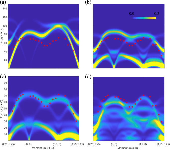
The color maps represent calulated spin wave of La3Ni2O7−δ with (a) δ = 0 (b) δ = 0.25 with an ordered oxygen vacancy distribution. c δ = 0.25 with an ordered oxygen vacancy distribution and all J‘s scaled by 0.83. d δ = 0.25 with a random distribution of splitted J‘s. Red dots represent experimental RIXS data in ref. 35.
Discussions
It is worth emphasizing that, given the complexities of dealing with correlated electrons, our study may only provides a semiquantitative analysis of the magnetic properties of La3Ni2O7−δ. The calculated magnetic moment appears larger than the experimental observed ones, with even larger values with increased U. However, based on our calculations, the presence of oxygen vacancies may introduce magnetic noncollinearity and spinless charge sites, which can lower the overall magnetic moments, bringing our results closer to the experimental observations. In this context, although La3Ni2O7−δ may also exhibit zero-point quantum fluctuations similar to those observed in 214 nickelates59,60, which could also help to reduce both the magnetic moment and the spin wave dispersion energy spread, we believe that our DFT + U calculations, combined with classical MC simulations still provide a reasonable interpretation for the magnetic properties of La3Ni2O7−δ.
Our results indicate that the TSDW and spin wave excitation energies are sensitive to the concentration of oxygen vacancies. At first glance, these conclusions appear to contradict experimental findings, where TSDW is consistently measured around 150 K across various samples. However, as shown in refs. 29,45, the distribution of oxygen vacancies in experimental samples is highly inhomogeneous. For instance, δ varies from approximately 0.04 to 0.32 in different regions of a single sample used in ref. 45. A plausible speculation is that the bulk volume of different samples has a similar moderate δ value, e.g., δ ~ 0.20 as observed in ref. 45, which supports a quasi-long-range magnetic ordering with a wave vector of (0.25, 0.25), resulting in a consistent TSDW. The discrepancies lie in the vacancy distribution in other regions. High-δ regions can induce spin-glass-like short-range orders at low temperatures, preventing the formation of long-range orders across the entire sample. Conversely, regions with smaller δ can exhibit magnetic ordering up to higher temperatures. This picture aligns with NMR observations, where critical spin fluctuations in regions away from oxygen vacancies persist up to 200 K, while below 50 K, glassy spin dynamics are observed29.
In conclusion, our calculations reveal strong nearest neighbor interlayer interactions, with amplitudes one order of magnitude larger than the other interactions. For δ = 0, our calculations favor the DSS phase with a (0.25, 0.25) in-plane modulation vector as the magnetic ground state. Oxygen vacancies effectively turn the Ni magnetic moments in the vicinity into charge sites. Therefore, with moderate δ values, our theoretical SDW phase is found to possess characteristics of both the DSS and the SCS, maintaining (0.25, 0.25) as the dominant modulation vector. This picture may provide a natural explanation to reconcile the seemingly contradictory experimental findings that both the DSS and the SCS are proposed as candidates for the SDW phase. At high concentrations of oxygen vacancies, such as δ = 0.5, we anticipate a short-range ordered ground state with spin-glass-like magnetic structures, leading to the destruction of the (0.25, 0.25) modulation vector. The presence of oxygen vacancies also lowers the TSDW due to the dilution of dominant exchange interactions. Notably, the magnetic ordering induces concurrent charge and orbital ordering, facilitated by spin-lattice coupling under the low-symmetry magnetic phase. Moreover, we find that the effect of a random distribution of oxygen vacancies may need to be considered to obtain a spin wave spectrum consistent with experiments. We further provide a plausible explanation for the experimental observations that the measured TSDW seems not sensitive to different samples and the lack of direct evidence for long-range magnetic ordering.
Note added: We notice two related works on the SDW of La3Ni2O7−δ41,42, which were posted around a week prior to our first submission. The two works focus on both the SDW under ambient pressures and high pressures, but without considering oxygen vacancies, while our work focus on the SDW under ambient pressures and the impact of oxygen deficiencies on the magnetic properties.
Methods
DFT + U and HSE06 calculations
First-principles calculations are carried out with the Vienna ab initio Simulation Package (VASP)61,62. We use the Perdew Burke-Ernzerhof functional with a spin-polarized generalized gradient approximation (GGA). The projector augmented-wave (PAW)63 method with a 550 eV plane wave cutoff is employed. The spin-polarized GGA is combined with onsite Coulomb interactions38 included for Ni 3d orbitals (GGA + U)1,8. The scheme is implemented using effective on-site Hubbard U parameter Ueff = U − J, where J is fixed to J = 1.0 eV. We use experimental lattice parameters, with the atomic positions fully optimized until the forces on each atom are reduced to less than 0.01 eV/ Å. For HSE0664,65,66,67,68,69 calculations, we employ the atomic-orbital-based ab initio computation at UStc (ABACUS) code package70,71, which makes use of the SG15 optimized norm-conserving Vanderbilt-type (ONCV) pseudopotentials72,73 and the so-called “DZP-DPSI”74 numerical atomic orbital basis sets.
Heisenberg exchange interactions and MC calculations
Utilizing the Wannier90 code75, we derive a tight-binding model employing maximally localized Wannier functions associated with La d f orbitals, Ni d orbitals, and O s p orbitals. Subsequently, the TB2J package76 is employed as a postprocessing tool to compute the Heisenberg exchange interactions based on the magnetic force theorem.
To construct the tight-binding model, our calculated DOS reveals that the d and f orbitals of La, the d orbitals of Ni, and the s and p orbitals of O contribute around the Fermi level (see Fig. S1 in Supplementary Note 2 of the supplementary materials). Therefore, the projection block includes these orbitals, defining a set of localized functions used to generate an initial guess for the unitary transformations. A broad frozen energy window spanning − 6 to 4 eV is employed to accurately capture the higher energy conduction bands, with the projection centers serving as reference points during the Wannierisation procedure. The orbital spreads are converged to less than 1 Å2 for the d orbitals, less than 2 Å2 for the s and p orbitals, and less than 5 Å2 for the f orbitals. The contribution of La’s f electrons to the Fermi surface is minimal. Therefore, it has a negligible effect on our calculation of the exchange parameters. The final Wannier-interpolated band structures are in good agreement with DFT-calculated band structures. (See Fig. S2 in Supplementary Note 2 of the supplementary materials)
The magnetic phase diagrams are obtained using MC simulations. Due to the complexity of frustrated interactions, traditional serial-temperature MC methods are often insufficient for sampling. Therefore, we employ the replica-exchange MC method43,44, where multiple replicas are simulated concurrently across a range of temperatures, enabling configurational exchanges between them. This approach allows higher-temperature replicas to facilitate broad phase space exploration for the lower-temperature replicas, helping to avoid trapping in local energy minima. In our simulations, each MC sweep includes attempts over all variable states. The MC simulations for the cases with zero vacancy and ordered vacancies are performed with a 16 × 16 × 2 superlattice with 1,000,000 MC steps for statistics at each temperature. We perform the simulations over a temperature range from 1 to 300 K, adjusting temperatures to maintain an exchange rate of approximately 20% between neighboring replicas. For each temperature, an initial 100 sweeps are conducted to equilibrate the system.
Oxygen vacancies simulation
Oxygen vacancies are simulated by removing the corresponding number of oxygen atoms from a La3Ni2O7 supercell. For magnetic moment calculations, we employ a 96-atom supercell. Experimentally synthesized La3Ni2O7 samples are commonly found to contain oxygen vacancies, with δ typically ranging from 0 to 0.529,31,39,45,46 Therefore, to reduce computational cost from the supercell approach, exchange interactions with oxygen vacancies are computed only for δ = 0.25 and δ = 0.5 using a 48-atom supercell, where removal of one oxygen atom yields δ = 0.25. In direct DFT calculations, a symmetric distribution of vacancies is adopted to mimic vacancies in real samples.
MC calculations with disordered oxygen vacancies
To further explore the magnetic phase diagrams in La3Ni2O7, we conduct additional calculations using the calculated exchange interactions J’s and MC simulations43,44. Given that the calculated J’s indicate weak interactions between different bilayers, we simplify the calculations by focusing on a single bilayer. We first construct an 8 × 8 bilayer structure containing 128 Ni atoms. To simulate the disorder of oxygen vacancies, we randomly select a certain number of Ni pairs to be non-magnetic (charge). For instance, for δ = 0.25, we randomly select 16 out of 64 Ni pairs to be non-magnetic. We then set all J’s directly involving charge sites to zero. We perform simulations for a range of δ values, with selected simulated TSDW and magnetic ground states shown in Supplementary Note 6 FIG. S8. In the MC simulations with disordered vacancies, we use a bilayer with 32 × 32 × 1 superlattice, which contains a total of 2048 Ni atoms.
Magnetic excitation spectra simulations with a random splitting of J’s
To better simulate the effects of random oxygen vacancies, we group the original 12 J’s values into respective pools and randomly select bonds from each pool, assigning these values to the 48 J’s (derived from the original 12 J’s). For example, ({J}_{2}^{0.25}) to ({J}_{5}^{0.25}) are derived from J1 in La3Ni2O7, with their coordination numbers all being 4 in a supercell containing 32 Ni atoms. We randomly select four bonds as ({J}_{2}^{0.25}), another four as ({J}_{3}^{0.25}), and so forth, resulting in a reclassified set of ({J}_{2}^{0.25}) to ({J}_{5}^{0.25}). For computational convenience, we focus on the major interactions, redistributing J1 ~ J7 and J12. This approach results in a random splitting of the J’s values, better reflecting the characteristics of random oxygen vacancies. Through quench optimization of the magnetic structure, we determine the magnetic ground state in the random scenario using a 2 × 2 × 1 supercell and obtain the corresponding theoretical spin wave.


Responses