Pairing at a single Van Hove point
Introduction
The ability to create and manipulate two-dimensional (2D) or strongly anisotropic 3D electronic materials led to an increased interest in the theory of systems in which the Fermi energy is at or near a Van Hove (VH) singularity of the electronic density of states1. Examples are doped graphene2,3,4,5, a wide range of moiré materials6,7,8,9,10,11,12, metallic Kagome systems13,14,15, as well as the ruthenate oxides Sr3Ru2O7 in an external magnetic field16, Sr2RuO4 under uni-axial compressive strain17,18,19,20 and twisted di-chalcogenides21. Studies of these materials extended earlier theoretical analysis of VH singularities in cuprate and other superconductors22,23,24,25,26,27,28,29,30,31,32,33,34.
In the analysis of the impact of VH singularities, two cases should be distinguished: In the first case, illustrated in Fig. 1a, there are several symmetry-related VH points that simultaneously cross the Fermi energy. In this situation, scattering events with large transferred momentum that connect different VH points are crucial. These processes often lead to density-wave instabilities, which trigger superconductivity nearby in the phase diagram via some version of the Kohn–Luttinger mechanism35,36,37,38. In the second case, shown in Fig. 1b, there is a single VH point at the Fermi level. Such a situation occurs in systems with low symmetry, including strained materials, where the application of large uni-axial stress reduces the number of allowed symmetry operations. A prominent example is Sr2RuO4, where stress along the Ru-O-Ru bond direction moves one of the VH points of the tetragonal system to the Fermi energy, while the other is pushed away from it17,18,19,20.
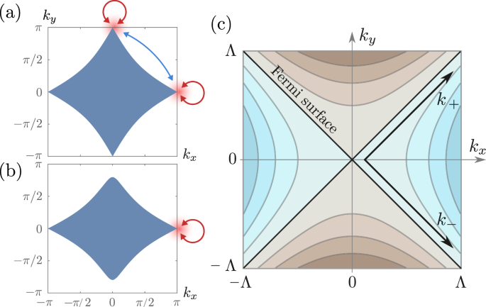
Fermi surface of a system with (a) two Van Hove points, and (b) a single Van Hove point at the Fermi energy. The shaded area shows the occupied states, and arrows illustrate the dominant interactions. c Iso-energy contours near the Van Hove point described by Eq. (4). Blue (brown) color indicates the occupied (unoccupied) states. The Fermi surface for the extended Van Hove point of Eq. (5) is the same, while the iso-energy contours will be different, with flatter bands near the Fermi energy. The coordinates ({k}_{pm }=({k}_{x}pm {k}_{y})/sqrt{2}) are extensively used throughout the text, where we consider gap functions that depend on only one of these coordinates, i.e., Δ(k+) or Δ(k−).
In addition to ordinary VH points, where the density of states in 2D diverges like a logarithm, extended VH points have recently been discussed extensively6,7,8,9,10,11,39. In this case, the density of states diverges by a power law due a saddle-point that is less dispersive than the ordinary quadratic one. In refs. 7,10 a classification of such extended singularities was given and it was shown that some extended VH points can be reached by solely varying a single parameter in the Hamiltonian. In ref. 39 it was argued that both ordinary and higher-order VH points are present for a model of fermions on a honeycomb lattice at different dopings.
For a single, ordinary or extended VH point, a Stoner-type analysis suggests a ferromagnetic instability at arbitrarily small interaction, due to the divergent density of states12,30. However, no such instability was detected in renormalization group (RG) studies8,11. A potential other instability is towards superconductivity, but it was also not detected in RG. The authors of ref. 8 argued, based on their RG study, that the ground state of a system with a single extended VH point does not possess a ferromagnetic or superconducting order, but rather is a particular non-Fermi liquid, dubbed a supermetal, in which the quasi-particle weight vanishes by a power-law as one approaches low energies.
In this paper, we consider the behavior of a system of fermions with repulsive interaction and a single ordinary (extended) VH point in 2D with logarithmic (power-law) divergence of the density of states by going beyond RG. We argue that the tendency towards a ferromagnetic Stoner instability likely remains suppressed, also the analysis becomes more nuanced, and the ferromagnetic susceptibility does go up with decreasing temperature, consistent with Quantum Monte Carlo data40. However, a superconducting instability does develop once we go beyond the conventional one-loop RG treatment, which accounts for the leading logarithms, and include the subleading ones. We argue that the superconducting order parameter is odd-parity and spin triplet. For an ordinary VH point, we obtain for the superconducting transition temperature
Here, g is the dimensionless coupling constant to be defined below, γ and μ are of order one, and ({T}_{0}=frac{{Lambda }^{2}}{2m}), where m is the curvature of the quadratic saddle-point dispersion around a VH point and Λ is the upper momentum cutoff of the theory. The functional form of Tc is the same as in BCS theory, but the analogy is a superficial one as in our case the effective interaction and the fermionic density of states are both logarithmically singular. The leading logarithms (the ones captured within the RG treatment) however cancel out leading to no pairing instability within RG. Beyond the leading logarithmic approximation, the product of the fermionic density of states and the attractive pairing interaction reduces to a constant. This leads to BCS-like form of Tc in Eq. (1).
For an extended VH point, we obtain
where ϵ is the exponent that determines the divergence of the density of states, ρ(ω) ∝ ∣ω∣−ϵ. We emphasize that Tc of an extended Van Hove point is no longer exponentially small despite that we again need to go beyond RG to obtain pairing. This is the consequence of the fact that is that for a power-law behavior of the density of states, the corrections to RG are of the same order as the terms kept in the RG (see, e.g., ref. 11) and hence even beyond RG the product of the fermionic density of states and the attractive pairing interaction remains singular. We emphasize that Tc gets strongly enhanced when ϵ increases and it is furthermore cutoff-independent as the dependence on Λ cancels out between T0 and g.
With respect to supermetal of ref. 8, our result indicates that such a state describes system behavior over some temperature and energy range, but at lowest temperatures or energies the system eventually becomes unstable against triplet superconductivity.
Solving the gap equation for T ≲ Tc, we find that the pairing state is highly non-local with an unusual momentum dependence of the Cooper-pair wave function. It changes sign under k → − k as required for odd-parity triplet pairing. However, the momentum regime, where the gap is linear in k, turns out to be extremely small, of order δk ~ 2mTc/Λ in the case of an ordinary VH point. Nodal excitations should therefore be hardly visible in thermodynamic measurements such as the specific heat, the Knight shift or the superfluid stiffness.
We also analyze the role of pairing fluctuations. The results Eqs. (1) and (2) are mean-field transition temperatures. For a spin-singlet superconductor, the actual transition at TBKT≤Tc is of Berezinskii–Kosterlitz–Thouless (BKT) type41,42 into a charge-2e state with algebraic order (power-law decay of superconducting correlations). For a 2D spin-triplet state, a charge-2e order survives in the presence of spin–orbit interaction. In its absence a spin-triplet order is additionally suppressed by fluctuations in the spin sector of the superconducting order parameter43,44. However, there exists a BKT transition into to a charge-4e state, in which two triplets bind into a singlet. In either case, the onset temperature for the algebraic superconductivity is comparable to the mean-field Tc, given in Eqs. (1) and (2).
Results
The model
We consider a system of interacting electrons with dispersion εk and Hubbard repulsion U:
where ψkα annihilates an electron with momentum k and spin α. We measure the momenta relative to the VH point, assumed to be time-reversal symmetric, and focus on the case where εk=0 = 0, i.e., the VH point is right at the Fermi level. We comment on the behavior upon tuning the Fermi energy away from the VH point in Discussion.
For an ordinary VH point the electronic dispersion is
An anisotropy between kx and ky, expected for a VH point located away from the center of the Brillouin zone, can be eliminated by an appropriate re-scaling of momenta. The quadratic dispersion in Eq. (4) gives rise to a logarithmically diverging density of states (rho (omega ) sim mlog (frac{{Lambda }^{2}}{mvert omega vert })), where Λ is the momentum cutoff – the highest momentum, up to which Eq. (4) is valid.
For an extended VH point, we follow earlier works27,29,31,32 and consider the dispersion in the form
where n ≥ 2. Now the density of states diverges by a power-law (rho left(omega right) sim {A}^{epsilon -1}{leftvert omega rightvert }^{-epsilon }) with ϵ = 1 − 2/n ≥ 0. In this paper, we focus on the dispersion Eq. (5), but note that other extended VH singularities are possible, e.g., with different powers for the two components of k6,7,8,9,10,11.
A potential Stoner instability
We begin with the discussion of a potential instability towards ferromagnetism. At a first glance, ferromagnetism near a single VH point is a natural option30, as this is a q = 0 instability, and it develops for a repulsive interaction between fermions. Within the random phase approximation (RPA), the instability occurs when the dimensionless interaction—the product of U and the density of states—reaches a certain finite value. In an ordinary metal with a finite density of states, this requires that U exceeds a threshold value. For the VH case, however, the density of states is divergent. Within RPA, the ferromagnetic Stoner condition is then satisfied already for an arbitrarily weak interaction. However, the same divergence of the density of states gives rise to singular corrections to RPA, which forces one to go beyond RPA.
Whether or not a Stoner instability develops beyond RPA can be detected by computing the static and uniform magnetic susceptibility χ, i.e., the limit q → 0 of the static susceptibility χ(q, ω = 0). This susceptibility can be obtained by either introducing an infinitesimal magnetic field and computing the magnetization or by introducing an infinitesimal bare ferromagnetic order parameter, dressing it by interactions, and computing the ratio of the fully-dressed and the bare order parameters. In the diagrammatic analysis, the second approach is easier to implement. The bare order parameter M0 is represented as a two-particle vertex, and the dressed one M is obtained by renormalizing this vertex by interactions. This is illustrated in Fig. 2a.
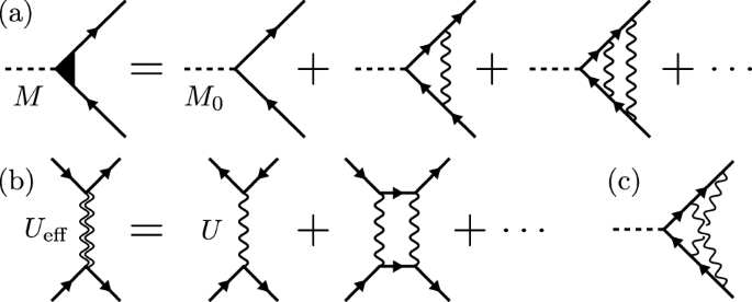
a Ladder series in the particle-hole channel [Eq. (6)]. b Series of particle-particle diagrams [Eq. (8)] which renormalize the interaction. c A diagram, generated by inserting a particle-particle renormalization into the particle-hole ladder series. At a Stoner transition, the diagrammatic series from M/M0 must sum to infinity; see text for further details.
For definiteness, we consider a single ordinary VH point. The particle-hole polarization bubble at a VH point is logarithmically singular: ({Pi }_{{rm{ph}}}=frac{m}{2{pi }^{2}}log frac{{T}_{0}}{T}) with T0 given below Eq. (1).
Within RPA, the dressed M is obtained by summing up ladder series of particle-hole renormalizations of M0. This summation yields
The susceptibility M/M0 diverges at UΠph = 1, i.e., at T = TFM satisfying ({lambda }_{0}log frac{{T}_{0}}{{T}_{{rm{FM}}}}=1), where
The ferromagnetic transition temperature TFM is finite no matter how small U is.
Beyond RPA, a simple experimentation shows that the most relevant contributions to M come from the crossed diagrams (Fig. 2c), which represent insertions of particle-particle renormalizations into the particle-hole channel. At zero total momentum and zero total frequency, a particle-particle polarization bubble ({Pi }_{{rm{pp}}}=frac{m}{2{pi }^{2}}{log }^{2}frac{{T}_{0}}{T}) diverges as ({log }^{2}) due to an additional Cooper logarithm. In RG calculations8,11, one assumes that this expression is still valid for the crossed diagram even though the total momentum and the total frequency in Πpp are finite. Within this assumption, one can compute the ladder series of particle-particle renormalizations of each term in Eq. (6) and find that they effectively replace U by
Substituting Ueff instead of U into Eq. (6), we find that the Stoner condition becomes
There is no solution of Eq. (9) at small λ0 because the suppression of λ0 by fluctuations in the particle-particle channel is stronger than the enhancement of λ0 in the particle-hole channel.
We went beyond RG and verified the accuracy of the RG calculation. For this, we explicitly evaluated the renormalization of U from the two-loop crossed diagram in Fig. 2c using the expression for Πpp at a finite total momentum and a finite frequency. We found that the renormalization of U from the two-loop crossed diagram is somewhat smaller than in the RG analysis, and the actual Ueff is
where b ≈ 1.88. The details of this analysis are summarized in Supplementary Note 1, where we determine the coefficient b numerically and show analytically that the naively expected ({log }^{2}frac{{T}_{0}}{T}) contribution vanishes due to a cancellation of two terms that individually scale as ({log }^{2}frac{{T}_{0}}{T}). We show that keeping the frequency dependence of Πpp is crucial for this cancellation.
Given that the leading term in Ueff cancels out, it is a-priori unclear how to re-sum the diagrams for Ueff and whether it is even justified to restrict with maximally crossed diagrams. If we assume that higher-order crossed diagrams form a geometrical series, we find ({U}_{{rm{eff}}}=U/(1+b{lambda }_{0}log left({T}_{0}/Tright))), which replaces Eq. (9) for the condition for the Stoner instability by
Since b > 1, one still finds that there is no Stoner instability. This argument is, however, a suggestive one, and whether there is a Stoner instability at a single VH point remains an open question. In what follows, we will assume that no ferromagnetic instability takes place and analyze a potential pairing instability.
Pairing instability
We now show that there is a pairing instability for the cases of both, the ordinary and the extended VH point. In order to theoretically detect it one has to go beyond the usual one-loop renormalization group treatment and include not only the leading logarithms, which cancel out, as we will see, but also the subleading ones. We will show that the pairing mechanism in our case is of the Kohn–Luttinger type, but is nevertheless different from the conventional Kohn–Luttinger scenario. In the latter, the screening of a repulsive Hubbard-type interaction U generates an attractive pairing interaction in the spin-triplet channel with dimensionless coupling constant
which gives rise to a BCS-type pairing instability. For an ordinary VH point, this would give rise to ({T}_{c} sim {T}_{0}{e}^{-1/sqrt{g}}) originating from (g{log }^{2}({T}_{0}/{T}_{c})=1), where one logarithm is a Cooper one and the other is due to the VH singularity in the density of states; we remind that T0 was introduced below Eq. (1). Such a result holds for a Fermi surface without VH points when the attractive pairing interaction is a logarithmically singular function of the frequency transfer45,46. In our case, the attraction in the spin-triplet channel does appear due to screening by particle-hole pairs and is of order U2. However, the effective pairing interaction ({Gamma }_{alpha beta gamma delta }left({boldsymbol{k}},-{boldsymbol{k}},{boldsymbol{p}},-{boldsymbol{p}}right)), where k and p are relative to the VH point, is strongly momentum dependent in the triplet channel and is reduced when one momentum is much smaller than the other one. This effectively eliminates the Cooper logarithm leaving only the one from the density of states. As a result, we will find that Tc is given by Eq. (1). The same holds for a higher-order VH point. In this case, there is no exponential dependence of Tc on g but Tc is still reduced compared to that in the conventional Kohn–Luttinger scenario.
A generic recipe for the analysis of potential pairing mediated by nominally repulsive electron-electron interaction is to consider an irreducible pairing vertex
instead of the bare U because Γ rather than U appears in the gap equation47. The irreducible pairing vertex is the anti-symmetrized interaction with zero total incoming and outgoing momenta, dressed by the renormalizations outside of the particle-particle channel, i.e., by processes which in a diagrammatic representation have no cross-sections with two fermionic propagators with opposite momenta. To second order in U, the static irreducible vertex takes the form48
The underlying processes are shown in Fig. 3, where ({Pi }_{{rm{ph}}}left({boldsymbol{k}}right)) is the static particle-hole polarization bubble.
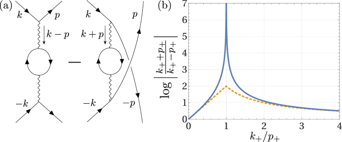
a Interaction vertex ({Gamma }_{alpha beta gamma delta }left({boldsymbol{k}},{boldsymbol{p}}right)) of Eq. (14) at second order in U, dressed by particle-hole excitations. Solid lines stand for fermions, which give rise to the bubble Πph. The wiggly line stands for the local interaction U. b The function (log leftvert frac{{k}_{+}+{p}_{+}}{{k}_{+}-{p}_{+}}rightvert), which determines the triplet component of Γαβγδ(k, p) for k− = p− = 0, as a function of k+/p+. The interaction gets weak whenever one of the two momenta is small. The blue solid line is the actual function, while the orange dashed line is an approximate expression based on Eq. (47).
The restriction to second order in U may seem questionable as in the previous section we argued that the coupling in the particle-hole channel is reduced, to the extent that no Stoner instability takes place. We will show, however, that the typical momenta k and p, responsible for pairing, are comparable to the cutoff Λ. For such momenta, the suppression of the coupling by crossed diagrams is small and can be neglected.
Pairing at the ordinary VH point
The gap equation for the ordinary VH point takes the conventional form
Here Zp is the inverse quasi-particle weight, related to the fermionic self-energy by ({rm{Sigma }}left({boldsymbol{k}},omega right)=-iomega {Z}_{{boldsymbol{k}}}). It is convenient to rotate the coordinate system by π/4 and introduce (rm{k}_{pm }=frac{1}{sqrt{2}}({rm{k}}_{rm{x}}pm {rm{k}}_{rm{y}})) and (rm{p}_{pm }=frac{1}{sqrt{2}}(rm{p}_{x}pm rm{p}_{y})). The Fermi surface around a VH point is specified by either p+ = 0 or p− = 0, see Fig. 1c. In these notations33,34
The gap equation can be split into two decoupled equations for the singlet and triplet components, respectively, by expressing the gap function as
The bare interaction U shows up only in the singlet channel, whereas the dressed ({Gamma }_{alpha beta gamma delta }left({boldsymbol{k}},{boldsymbol{p}}right)) of Eq. (14) contains both singlet and triplet components. No solution for ({Delta }_{s}left({boldsymbol{k}}right)) exists in the singlet channel, because the dressed pairing vertex remains repulsive. In the triplet channel, the gap equation takes the form
with i = x, y, z. When solving the gap equation, we choose an arbitrary quantization axis in spin space and omit the index i. We get back to this issue when we discuss superconducting fluctuations.
In terms of k± and p±, the pairing vertex is the sum of two terms
We see that one of the terms vanishes when either k+ = 0 or k− = 0. This allows to search for Δ(k) which depends only on one of the coordinates, i.e., (Delta left({k}_{+}right)) or (Delta left({k}_{-}right)). Even if there exist more complicated solutions, finding a solution of this kind is enough to establish a lower bound for the superconducting Tc. For definiteness, below we consider (Delta ({boldsymbol{k}})=Delta left({k}_{+}right)) and (Delta ({boldsymbol{p}})=Delta left({p}_{+}right)). Under this assumption, we can perform the integration over p− at the outset and obtain
The function
determines the effective density of states for momenta transverse to the Fermi surface. The expression is valid when (frac{{p}_{+}Lambda }{2mT},gg ,1), setting the temperature dependent lower cutoff for p+ at 2mT/Λ. The upper cutoff is at p+ = Λ. For g → 0, (Kleft({p}_{+}right)to log frac{{p}_{+}Lambda }{2mT}).
It is convenient to introduce dimensionless variables (bar{p}=frac{Lambda {p}_{+}}{2mT}) and similar for (bar{k}), and (bar{Lambda }=frac{{Lambda }^{2}}{2mT}). In these variables, the gap equation takes the form
with
We solved this equation numerically and obtained Tc(g) and (Delta (bar{k})). In Fig. 4 we plot (gYleft(gright)) with
as function of the coupling constant g. We find that at small g the behavior is well described by a linear relation (glog frac{{T}_{0}}{{T}_{c}}=(1+mu g)/gamma) with
This yields the transition temperature given in Eq. (1). In Fig. 5, we show the momentum dependence of the gap function (Delta (bar{k})) extracted from the numerical solution. (Delta (bar{k})) is odd under (bar{k}to -bar{k}) as required for an odd-parity triplet state. The momentum dependence is non-monotonic with a maximum at an intermediate momentum, which scales with Λ but numerically is much smaller than Λ. The linear dependence of (Delta (bar{k})) on (bar{k}) holds at even smaller momenta below the maximum.
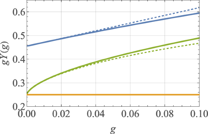
The blue dashed line is a fit to (1 + μg)/γ with γ and μ given in Eq. (25). This dependence of gY(g) leads to Eq. (1) for Tc(g). The green lines are the solutions of the gap equation without self-energy, which we discuss in Supplementary Note 2. The solid green line is the full numeric solution while the dashed line is the approximate analytic solution. The orange line is the zero-order approximate result, Eq. (27). Recall that larger Y(g) correspond to smaller Tc.
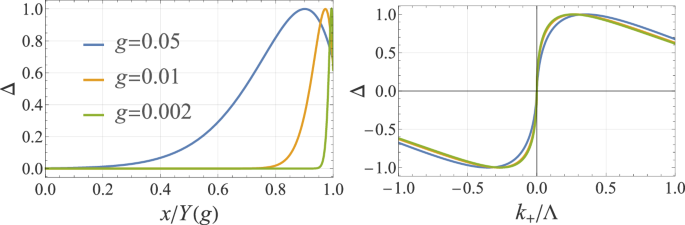
Such a gap function develops infinitesimally below Tc. The gap function is normalized to its maximal value. Left panel: Δ(x) as a function of x/Y(g), where (x=log left(frac{Lambda {k}_{+}}{2mT}right)) and (Y(g)=log {T}_{0}/{T}_{c}(g)). Right panel: Δ(k+) as function of k+/Λ. Notice the non-monotonic behavior of the gap function with a steep slope at small momenta.
Analytical treatment at the ordinary VH point
We also analyzed the gap equation analytically. The analysis is somewhat involved, particularly when we include fermionic self-energy. Yet, the full analytical consideration yields the same expression for Tc as Eq. (1) with quite similar values of γ and μ. To gain physical insight into the origin of the pairing beyond RG, below we present the results of an approximate analytical treatment, in which we approximate (Kleft(bar{p}right)) in (21) by a constant (log bar{Lambda }) and pull it out of the integral over (bar{p}) in Eq. (22). This approximation holds when we expand the logarithmic term in the r.h.s. of (22) to first order in g (which effectively amounts to neglecting the fermionic self-energy) and approximate (bar{p}) by (bar{Lambda }). The gap equation then reduces to
where ({g}^{* }=glog bar{Lambda }) is the effective coupling constant.
The solution procedure for Eq. (26) is described in Methods section. We find the critical temperature
which is shown as the orange line in Fig. 4. We emphasize that the solution captures the two key features of the pairing in our case. First, the Cooper logarithm is suppressed because the pairing interaction in Eq. (19) gets suppressed when an internal momentum is larger than an external one and vice versa. Taken alone, this suppression would impose a threshold value for pairing, i.e., Tc would be nonzero only for g larger than some critical value. Second, the large density of states, encoded in the phase space of transverse momenta that determine the function (K(bar{k})) in Eq. (23), compensates for the weak pairing: it is the effective coupling constant ({g}^{* }=glog left[{Lambda }^{2}/(2mT)right]) that must reach a threshold. Because g*(T → 0) → ∞, the threshold condition is satisfied at a finite Tc for any g. The combination of the two effects yields Tc, which has the same form as the BCS expression, albeit for a different reason.
There is a certain analogy between the solution for Tc and the gap function in our model and in the model with the singular dynamical interaction between fermions, χ(Ωm) ∝ 1/∣Ωm∣γ (the γ model)49,50,51,52,53. In both cases, the integral equation for the gap function can be reduced to the differential equation with a marginal kernel, whose solution yields a power-law dependence of the gap function x±a (x is a momentum in our case and a frequency in the γ model), where a depends on T in our case ((a=sqrt{1-4{g}^{* }})) and on γ in the γ − model. As long as the exponent a is real the potential solution Δ (x) = xa + bx−a does not satisfy the two boundary conditions, hence there is no superconductivity. A non-zero solution develops when the exponents ± a merge. In this case, besides a constant, there appears the second solution (log x). The candidate solution (Delta (x)=1+blog x) satisfies the two boundary conditions, which fix the value of b, and hence is the actual solution of the linearized gap equation. This implies that a = 0 is the condition for Tc Also, in both cases the solution of the linearized gap equation exists even at 4g* > 1, as the end point of the infinite set of solutions of the non-linear gap equation.
In a more accurate analytical treatment in Supplementary Note 2, we expanded to second order in g in Eq. (21) and obtained a bit more complex differential gap equation, from which we extracted
with γr = 1.7544 and μr = 2.092 The functional form of (28) is the same as extracted from the numerical solution of the gap equation, and the values of γr and μr are reasonably close to numerical values in Eq. (25).
Comparison with Son’s model
It is also instructive to compare our result for Tc with the one for fermions away from VH singularity, but with an attractive logarithmic interaction. Such a model was originally solved by Son in the frequency domain45, see also ref. 46. In momentum space, the corresponding gap equation in our notations (bar{k}=k/Lambda) has the form
where (bar{Lambda }={Lambda }^{2}/(2mT)), as before. We also keep the notation g for the dimensionless coupling constant. At a first glance, the effect of logarithmic interaction is the same as from logarithmic density of states at the VH point (Eq. (22)). We show, however, that these two problems are rather distinct, because in our case the effective interaction (log leftvert frac{bar{k}+bar{p}}{bar{k}-bar{p}}rightvert), while generally of order O(1), is strongly reduced when one momenta is much smaller than the other one. This effectively eliminates the Cooper logarithm that emerges through (dbar{p}/bar{p}) in both Eqs. (22) and (29).
We find the transition temperature (see Methods)
Comparing this with Eq. (1), we find that Tc for the single VH point is smaller as it contains 1/g in the exponent as opposed to (1/sqrt{g}) in Eq. (30). The distinction is due to the form of the pairing interaction in the triplet channel. In the case of pairing at the VH point, the pairing strength alone is too weak to give rise to a Cooper instability. However, the enhanced phase space for scattering, which is a consequence of the logarithmic density of states, compensates for the weak interaction and yields, in the end, a BCS-type expression of the transition temperature.
Pairing at the extended VH point
Next, we analyze extended VH points with a dispersion relation given in Eq. (5) for small but finite power-law exponent ϵ that determines the density of states. We show in Supplementary Note 3 that the inverse quasi-particle weight in this case is given by
where the dimensionless coupling constant is now
Note that this g explicitly depends on the cutoff Λ. This will play a role when we consider the limit where g ≪ ϵ.
The gap equation can be written as
For the particle-hole bubble at small ϵ we find
and we introduced the function
Here, ({p}_{0}=frac{T}{A{Lambda }^{1+2epsilon }}) is the temperature-dependent lower cutoff of the theory.
We transform the gap equation into a differential equation as described in Methods, and solve the resulting equation in the limits where the ratio of the small dimensionless constants g and ϵ is either large or small. We express the critical temperatures using the logarithmic variable (Y(epsilon )=log frac{{T}_{0}}{{T}_{c}(epsilon )}), where T0 = AΛ2+2ϵ. In each case, we compare the analytical results with the numerical solution of the gap equation.
The limit ϵ ≪ g
In this limit, we compute the leading correction in ϵ/g to the expression for Tc for an ordinary VH point from first order perturbation theory for the Schrödinger equation, expanding the equation, the boundary condition, and the potential (Vleft(xright)) to linear order in ϵ. The resulting set of equations is then solved numerically and determines the correction δY defined as
The result for δY is shown in Fig. 6. When g is larger than g* ≈ 0.013, δY is negative, hence the superconducting transition temperature increases with ϵ. At smaller g < g*, δY > 0 and scales with g as 1/g2. The superconducting transition temperature decreases with ϵ as
where a = O(1). We emphasize that this Tc(ϵ) smoothly connects to Tc(ϵ = 0) at the ordinary VH point.
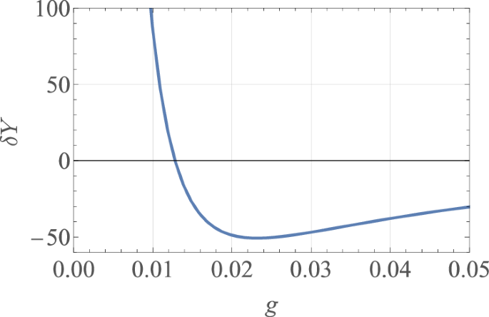
The sign of δY determines whether Tc for an extended VH point increases or decreases with ϵ. For a negative δY, Tc increases, for a positive δY it decreases. We see that δY is positive at very small small g and negative at larger g. The sign change occurs at g* ≈ 0.013. For small g, δY scales as 1/g2.
The limit ϵ ≫ g
We now show how the result for Tc gets modified in the opposite limit ϵ ≫ g. We set ϵ to be a number of order one and compute Tc by order of magnitude, keeping the explicit dependence on ϵ in the exponent, but neglecting the dependence on ϵ in the prefactor. For ϵ ≫ g, we can safely take the limit Λ → ∞ as all integrals are UV convergent. Evaluating the integral for K(p+) in Eq. (35) in infinite limits, we obtain
where x = p−/p+ and ({x}_{min } sim T/{T}_{epsilon }), where ({T}_{epsilon }=A{({p}_{+})}^{2(1+epsilon )}). Next, we assumed and verified that the relevant p+ in the equation for the pairing vertex are of order Λg1/(4ϵ). This allows us to express Tϵ ~ T0g(1+ϵ)/(2ϵ).
The integral over x in Eq. (38) converges in the UV limit, which allows us to set the upper limit of the integration over x to infinity. It is logarithmically singular in the IR limit and with logarithmic accuracy we obtain ({lambda }_{epsilon } sim log {T}_{epsilon }/T=log {T}_{epsilon }/{T}_{c}(epsilon )). In the differential gap Eq. (61), we now have (V(x)approx (1+epsilon )(1+epsilon -2{lambda }_{epsilon })={beta }_{epsilon }^{2}). The solution of Eq. (61) with such V is (bar{Delta }left(xright) sim {e}^{pm {beta }_{epsilon }x}).
A similar power-law solution (as a function of frequency) holds for a number of quantum-critical systems49 and Yukawa SYK-type models50,51,52. We verified that, like there, the solution, that satisfies boundary conditions, does not exist when βϵ is real, but emerges when βϵ becomes complex, and the onset of complex βϵ sets the value of Tc. In our case, βϵ becomes complex at λϵ = (1 + ϵ)/2, which for a generic ϵ is a number of order one. Using ({lambda }_{epsilon } sim log {T}_{epsilon }/{T}_{c}(epsilon )), we then find that
We see that Tc(ϵ) is not exponentially small in g. We also notice that Eq. (39) can be re-expressed, using (32), as
This last expression shows that Tc(ϵ) does not depend on the upper cutoff Λ (the Λ − dependencies in T0 and g cancel out) and in this respect is universal.
At a qualitative level, we found that the crossover from Tc for an ordinary VH point to the one for an extended VH point is captured by the interpolation formula
In the limit ϵ ≪ g, this reduces to (log {T}_{0}/{T}_{c}(epsilon to 0)=1/gamma g), in the opposite limit ϵ ≫ g, one recovers the universal power-law expression Tc(ϵ) ~ T0g(1+ϵ)/(2ϵ).
Numerical solution for extended saddle points
We also performed the integration over the transverse momenta in the function K(p+) in Eq. (35) numerically and solved numerically the gap Eq. (33) with this K(p+). We show the results in Figs. 7 and 8. In Fig. 7 we show the dependence of (Y(g,epsilon )=log (frac{{T}_{0}}{{T}_{c}(epsilon )})) on the coupling constant g. The distinct behavior for ϵ smaller and larger g is clearly visible. For ϵ > g the linear dependence of Y on (log g) demonstrates that the transition temperature Tc(ϵ) has the power law form Tc(ϵ) ∝ gα. The value of α is determined from the slope. The data are best described by ({T}_{c}(epsilon )propto {g}^{frac{1}{2epsilon }}), consistent with Eq. (39). For ϵ < g the behavior deviates from the power law. In Fig. 8, we show how the small ϵ behavior of Tc(ϵ) from Fig. 6 interpolates to the power-law behavior at larger ϵ. For g < g* = 0.013, the dependence of Tc(ϵ) on ϵ is non-monotonic, in agreement with our analytic findings.
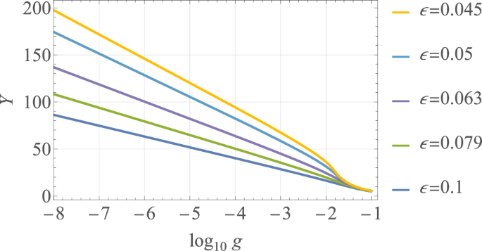
For ϵ > g we find power-law behavior Tc ∝ gα. The exponent α is determined from the slope of (Yleft(g,epsilon right)) vs (log g) and with high accuracy is (alpha approx frac{1}{2epsilon }), consistent with our analytical analysis. For ϵ < g the behavior deviates from the power-law dependence.
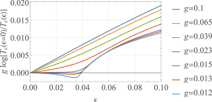
For g < g* = 0.013, the dependence is non-monotonic, consistent with our analytical results. For larger g, Tc(ϵ) monotonically increases with ϵ.
Pairing fluctuations, BKT transition and charge-4e superconductivity
We next discuss the statistical mechanics that we expect to emerge from our analysis.
The solutions discussed in the previous section formally belong to a two-dimensional irreducible representation (left(Delta left({k}_{+}right),Delta left({k}_{-}right)right)) of the point group. Hence, fluctuations of the order parameter might give rise to vestigial order with symmetry breaking of composite order parameters like nematic or time-reversal symmetry breaking states54. This is a consequence of the four-fold symmetric dispersions of Eqs. (4) and (5). However, the symmetry of a single VH point is usually lower and Eqs. (4) and (5) are the result of an anisotropic rescaling of momenta. This will lift the degeneracy of the two solutions and the triplet order parameter belongs to a one-dimensional representation of the point group.
For a 2D system, one usually expects a Berezinskii–Kosterlitz–Thouless (BKT) transition41,42 to a state with algebraic order and with finite superfluid stiffness. As discussed by Halperin and Nelson55, the resulting BKT transition temperature is very close to the mean field transition temperature that one obtains from the solution of the gap equation. The reason is that the threshold stiffness of the BKT transition is much smaller than the low-T stiffness of a weakly coupled superconductor. Hence vortex proliferation sets in only very near the mean field transition temperature. However, the BKT physics does not hold for a triplet superconductor without spin–orbit interaction. Fluctuations of such a state are governed by the three-component complex coordinate-dependent field ({boldsymbol{psi }}(x)={left({psi }_{1}(x),{psi }_{2}(x),{psi }_{3}(x)right)}^{T}) that describes long-wavelength variations of the pairing wave function
where ({Delta }_{i}left({boldsymbol{k}}right)) is the gap function discussed in the previous section. Fluctuations between components of ψ, i.e., fluctuations in the spin sector of the triplet state, destroy even an algebraic order due to the Hohenberg–Mermin–Wagner theorem56,57. In the notation ψ = ψ0neiθ where θ is the U(1) phase of the superconductor while the unit vector n describes spin fluctuations of the triplet state, algebraic order of ψ is suppressed by fluctuations of n.
The situation is different for a composite order parameter
which describes a charge-4e superconductor, in which two triplets form a singlet in spin space43,44. Since n2 = 1 it follows that
i.e., ϕ possesses only phase fluctuations, which allow a BKT transition. The extra factor 2 in the exponent in Eq. (44) allows for fractionalized vortices of the primary superconducting order parameter (the spin field heals the mismatch that forms at a fractional vortex, see ref. 58). The threshold stiffness for the BKT transition in a charge-4e superconductor is four times larger than that for a charge-2e superconductor, yet it is still much smaller than the zero temperature stiffness. Hence, the 4e BKT transition still occurs e very near mean-field Tc for the primary 2e order parameter. If spin–orbit interaction is present, the anisotropy in spin space suppresses fluctuations and allows charge-2e superconductivity with an algebraic order.
Discussion
In this work, we analyzed low-temperature instabilities of a system of fermions with a single ordinary or extended VH point at the Fermi level, in the limit of small electron-electron interactions.
We first considered the possibility of ferromagnetic order and argued that it likely does not develop because of strong reduction of particle-hole response in the q → 0 limit by particle-particle fluctuations.
We then analyzed pairing instabilities and explicitly demonstrated both, analytically and numerically, that a system with a single VH point at the Fermi level is unstable towards triplet superconductivity. The instability develops for both a conventional and a higher-order VH point, but Tc is much higher for a higher-order VH point in the regime ϵ > g, where it varies with the coupling constant g in a power-law fashion, as Tc ∝ g(1+ϵ)/(2ϵ). We showed that this Tc is a universal, cutoff independent quantity, determined by the band curvature and the local interaction.
The attractive triplet component of the pairing vertex comes from the Kohn–Luttinger type dressing of the pairing interaction by particle-hole fluctuations. Yet, we demonstrated that the mechanism for superconductivity is distinct from the usual Kohn–Luttinger one. In our problem, the attractive component of the vertex function is weak and, on its own, would not lead to a Cooper instability. However, the enhancement of the density of states near a VH point overcomes the smallness of the pairing vertex and gives rise to a BCS-like expression for Tc for an ordinary VH point and to power-law dependence of Tc on the coupling for an extended VH point.
As a consequence of this fundamentally non-BCS pairing mechanism, the transition temperature is expected to rapidly drop once the system moves away from a VH singularity under, e.g., a change of the chemical potential. Given the absence of a Cooper phenomenon, we expect that away from a VH singularity, superconductivity will develop only if the coupling exceeds a certain threshold. For any given g, there will be then a superconducting quantum critical point at some detuning. Similar behavior occurs for pairing at a critical point towards density-wave order and in SYK models49,50,51,52,53.
To illustrate this effect we compare Tc(μ) for our system and for a system with a constant attraction g and a logarithmic density of states, detuned by μ (a detuned version of the model discussed by Son). In the last case, the transition temperature is determined by
where ({T}_{c}(mu =0)propto {e}^{-pi /(2sqrt{g})}), see Eq. (30). For (leftvert mu rightvert, >, {T}_{c}left(mu =0right)), the effective coupling constant is reduced, yet Tc(μ) remains finite. For our problem, Tc(μ) is determined by
and remains non-zero only at (leftvert mu rightvert < {T}_{c}left(mu =0right)). For larger detuning from a VH point, Tc = 0. This sets a superconducting quantum critical point at ∣μ∣ ~ Tc(μ = 0). We illustrate this in Fig. 9.
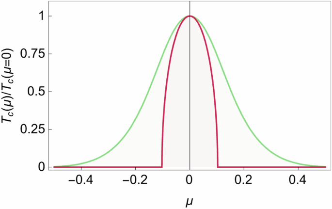
In the case of a constant attraction (green curve), the transition temperature, determined by Eq. (45), gets reduced upon detuning from the VH point, but remains finite.
We also discussed the role of critical fluctuations and argued that the transition temperature that we derived from the linearized gap equation is close to a BKT transition into an algebraic superconductor, which in the absence of spin–orbit interaction is a charge-4e superconductor made up of singlet bound states of triplet pairs, and in the presence of spin–orbit interaction is a charge-2e superconductor.
In our analysis, we concentrate on processes that are exclusively due to interactions between fermions at or near a VH point. It is important to keep in mind that some crucial physical processes may come from electronic states away from a VH point, particularly for transport phenomena20. For thermodynamic instabilities, the instability that we found here is, however, the leading one in the pairing channel in the limit of weak coupling.
A final note. In our analysis, we assumed that the dimensionless coupling g is small. How Tc evolves with g once g becomes O(1) is an issue for further study. We emphasize, however, that the most relevant effect of larger g is larger fermionic incoherence measured via the self-energy. Our results for Tc include the self-energy, both for ordinary and higher-order VH singularity. From this perspective, we expect that our formulas remain qualitatively valid even at g = O(1).
Methods
Analytical approximation for the ordinary VH point
To extract Tc in the approximation of Eq. (26), we follow refs. 46,49 and split the integral over (bar{p}) into the regimes (bar{p}, < ,bar{k}) and (bar{p}, > ,bar{k}) and in each regime use
We then obtain
Differentiating w.r.t. (bar{k}) we reduce Eq. (48) to a second order differential equation
with UV and IR boundary conditions
imposed by the original integral equation. For 4g* < 1 (i.e., at higher temperatures), the trial solution of Eq. (49) is
where e is a free parameter. However, we verified that one cannot find e that would satisfy both boundary conditions. Hence, the gap equation has no solution for g* < 1/4. For 4g* > 1 the trial solution is
where ϕ is a free parameter. The IR boundary condition now specifies ϕ to be the solution of (tan phi =-{left(4{g}^{* }-1right)}^{-1/2}), while the UV boundary condition yields
with integer l. Using (bar{Lambda }={Lambda }^{2}/(2mT)), we find that this equation determines a discrete set of critical temperatures Tc(l). The largest Tc corresponds to l = 1 and is the solution of (sqrt{4{g}^{* }-1}approx pi /log bar{Lambda }). Solving at small g, we obtain the critical temperature (27).
Solution of Son’s model
To solve Eq. (29), we split the integral over (bar{p}) in the r.h.s of (29) into regions (bar{p}, < ,bar{k}) and (bar{p}, > ,bar{k}), as we did before, introduce logarithmic variables (x=log bar{k}), (y=log bar{p}) as well as (Y=log bar{Lambda }), and convert (29) into the the differential equation
with boundary conditions ({Delta }^{{prime} }left(0right)=0) and (Delta left(Yright)=0). The solution in terms of the original variable (bar{k}) is
We see that (Delta (bar{k})) oscillates as a function of (log bar{k}) for any value of g, even infinitesimally small ones. This is in contrast to our earlier discussion, where an oscillating solution holds only for λ above the threshold. The IR boundary condition yields ϕ = lπ, with integer l, while the UV condition yields (cos left(sqrt{g}Yright)=0), i.e., (sqrt{g}Y=left(2l+1right)frac{pi }{2}). The transition temperature corresponding for each l is
The highest transition temperature is for l = 0, given in Eq. (30).
Differential gap equation at the extended VH point
The gap Eq. (33) for the extended saddle point can be transformed into a differential equation using a procedure analogous to that for the ordinary saddle point. The pairing kernel in Eq. (33) can be approximated as
with ({Pi }_{{rm{ph}}}^{{prime} }({k}_{+})=-frac{1}{4{pi }^{2}A}{leftvert {k}_{+}rightvert }^{-(1+2epsilon )}.)
Re-expressing the coupling in (33) in terms of the dimensionless g from (32), splitting the integration over p+ in into the ranges p+ < k+ and p+ > k+ and using Eq. (58), we re-express the gap equation as
Rescaling the gap function as
and introducing again the logarithmic variable
we obtain a Schrödinger-type differential equation
with potential
The boundary conditions are now given as
where (Y=log frac{Lambda }{{p}_{0}}=log frac{A{Lambda }^{2+2epsilon }}{T}) and T = Tc(ϵ). We study this equation analytically when ϵ ≪ g or ϵ ≫ g and solve it numerically for general ϵ and g.
Responses