Estimating emissions reductions with carpooling and vehicle dispatching in ridesourcing mobility

Introduction
With the ever-increasing number of cars on the roads, problems such as traffic congestion, environmental pollution, and energy consumption have increasingly impeded the rapid development of urban economies. Traditional taxi serves as an indispensable transportation mode, bridging the gap between public and private mobility due to their notable attributes of flexibility and accessibility. However, the taxi service identifies and serves passengers solely based on drivers’ experiences, which not only results in wasting time and resources but also exacerbates the problem of supply-demand imbalances1. In recent years, with the development of global positioning systems and smartphones, the emergence of ride-hailing services has transformed the landscape of the urban taxi industry1,2. By leveraging real-time passenger travel and vehicle location information, ride-hailing platforms achieve efficient and precise matching of supply and demand resources, effectively addressing the challenges where passengers search for available vehicles3,4. The ride-hailing platform receives travel orders and dispatches vehicles, simplifying the booking process by notifying the passenger of the assigned vehicle and estimated arrival time. Passengers can track the approaching vehicle in real-time, and drivers follow optimized navigation routes.
Although both ride-hailing services and traditional taxi services suffer from low seat utilization rates, ride-hailing services have the potential to leverage their internet-based features to facilitate shared rides among multiple passengers5. Carpooling is the practice of multiple passengers sharing a single vehicle for a common trip or destination, which is a highly effective approach to optimize travel efficiency, reduce traffic congestion, and decrease individual travel costs by distributing the travel expenses among the passengers. By promoting the widespread adoption of carpooling within the ride-hailing industry, it becomes possible to enhance vehicle seat utilization rates without necessitating an increase in the number of vehicles or alterations to existing road infrastructure. Consequently, this approach offers a viable means of improving the supply level of the taxi market by effectively utilizing the potential of available vehicle capacity6,7,8. Ride-hailing companies, e.g., DiDi Chuxing, Uber, and Lyft, have experienced rapid expansion in cities worldwide. As of the first quarter of 2024, Uber trips grew to 2.6 billion, ~28 million trips per day on average8. DiDi Chuxing platform saw a transaction volume of 3.75 billion rides, while ride volume in international markets grew to ~790 million rides9.
Ride-hailing platforms enable users to conveniently access information about available vehicles in their vicinity and pre-book rides through a mobile app. Moreover, to meet diverse and personalized travel needs, ride-hailing platforms have introduced various service modes, e.g. shared rides, premium services10,11,12. The advancement of ride-hailing has not only improved convenience and travel experiences for passengers but also reduced individual car ownership and usage. The convenient Internet payment and comfortable commuting experience have stimulated the public’s preference for ride-hailing services13. However, ride-hailing vehicles may operate in an empty state due to improper vehicle dispatching operations, leading to additional fuel consumption and detour distances14,15.
Carpooling is a means of transportation where at least two carpooling participants with similar itineraries, including route and schedule, share a car for at least a part of their journey. Carpooling is often considered beneficial in terms of congestion management, where two or more travelers with similar itineraries and time schedules share one vehicle so that the total number of vehicles on the roads is potentially reduced. Effective order matching and vehicle dispatching strategies improve the operational efficiency of ride-hailing services, reduce user waiting time, and decrease vehicle idle time, thus enhancing the service quality of ride-hailing services16. Santi et al.5 proposed a shareability network for modeling carpooling in ride-hailing services to maximize order-matching ratios. Results demonstrated carpooling trips is a possible way of reducing the negative impact of taxi services on cities, offering benefits such as reduced service costs, decreased emissions, and fare sharing. Kameswaran et al.17 conducted a study on Uber drivers and passengers, finding that passengers prefer to share rides with individuals who have similar personalities and even desire to engage in conversation during the journey. Besides, some passengers are willing to take a detour if special landmarks or scenic locations are included along the way.
Vehicle dispatching in ride-hailing services involves the allocation of available drivers and vehicles to incoming ride requests from passengers. Vehicle-dispatching strategies aim to minimize passenger waiting time18, maximize driver profit19, or balance supply and demand6. Vazifeh et al.6 proposed a matching algorithm based on the traffic network to fulfill total passenger travel demands intending to minimize the number of vehicles. Experimental results with real data showed that all orders can be served using only 70% of the vehicles. Seow et al.20 designed a distributed order dispatching system that minimizes the total waiting time of passengers. The proposed scheduling system uses a multi-agent method to achieve automatic taxi dispatching, and results showed a reduction of 33.1% in passenger waiting time and 26.3% in empty cruising time respectively. Potential order matching is utilized to improve seat utilization of ride-hailing vehicles, while dynamic vehicle dispatching is employed to improve vehicle utilization, thereby reducing empty cruising distances and pollution emissions.
As global environmental issues gain increasing prominence, the reduction of pollutant emissions has become a critical concern within the transportation system. Carpooling through ride-hailing services is increasingly recognized and valued for its role in reducing carbon emissions and protecting the environment1. Compared to traditional taxis and private cars, ride-hailing platforms make more efficient use of vehicle resources, reducing empty or partially loaded trips and lowering the carbon emissions per passenger. Besides, carpooling enables multiple individuals to share a single vehicle and it will make stops to pick up other riders. This service significantly reduces vehicle fleet sizes on the road, fostering resource sharing and conservation, thereby effectively lowering carbon emissions21,22. The optimization of route planning in carpooling services can be achieved to avoid redundant distances and fuel consumption23,24. Yu et al.25 evaluated the indirect environmental benefits of the shift to carpooling, where the estimated results show that ridesharing can achieve about 26.6 thousand energy savings and reduce CO2 and NOx emissions by ~46.2 thousand tons and 253.7 tons per year in Beijing city. Ride-hailing platforms encourage drivers to operate vehicles efficiently with order-matching and vehicle-dispatching algorithms to reduce CO2 emissions26,27.
An accurate estimated time of arrival (ETA) refers to the time prediction task when the vehicle is expected to arrive at a particular destination based on various factors such as current location, distance, and traffic conditions. Passengers submit the origin, destination, and desired departure time when using the ride-hailing service, but the arrival time for the upcoming trips at the destination is unknown. For ride-hailing platforms or drivers, precise ETA is crucial in deciding whether to accept an order and how to efficiently plan driving routes and schedules. Arrival time prediction tasks are influenced by complex traffic conditions, including temporal and spatial dependencies, and are susceptible to external factors such as weather and land use characteristics of pick-up/drop-off locations28. By utilizing prediction results, platforms can anticipate the time required for drivers to reach their destinations, enabling enhanced order allocation and optimization of vehicle dispatching29. By leveraging real-time traffic data and prediction models, the platforms consider potential congestion situations for order matching and vehicle dispatching, thereby providing passengers with more accurate and reliable services30,31,32.
With the advancement of artificial intelligence, emerging machine learning algorithms learn patterns and trends from a vast amount of historical data without the need for explicit estimation of vehicle travel time. Instead, they can leverage multiple factors to predict travel time such as passengers’ historical orders, current traffic conditions, departure time et al.33,34. Some scholars have applied deep learning methods for travel time estimation. Wang et al.35 proposed an end-to-end framework for travel time prediction. Complex factors, including spatial correlations, temporal dependencies, and external conditions (e.g. weather, traffic lights) are extracted by convolutional neural networks to integrate geographic information and utilized long short-term memory networks to extract temporal features. Besides, model interpretability is crucial in estimating travel time because it helps understand how various factors contribute to the prediction tasks. Explainable machine learning models provide clearer and more intuitive explanations of the results, enabling users to understand the contribution of each feature to the different prediction tasks and how the models utilize these features for forecasting36,37.
Online ride-hailing services face several challenges that impact their operations and user experience, including spatial-temporal imbalances in supply and demand, long detour distances, extended passenger waiting times, and increased carbon emissions. This study utilizes large-scale ride-hailing travel records data to estimate emissions reductions with order matching and vehicle dispatching optimization. A tree-based explainable machine learning model is established to dynamically predict the time for drivers to fulfill orders by transporting passengers to their destinations. Built upon dynamic arrival time prediction, the algorithm operates within a trip-based shareability network for potential order merging, increasing the matching success rate of carpooling services. Subsequently, an on-demand order-matching algorithm is designed to identify orders with similar origins and destinations. Dynamic vehicle dispatching is devised to optimize the utilization for servicing orders, and estimate carbon emissions reduction in various scenarios. This framework is illustrated in Fig. 1.

The framework includes the prediction of arrival time, potential order matching, and dynamic vehicle dispatching. It utilizes large-scale ride-hailing travel records to estimate emissions reductions in various scenarios of ridesourcing mobility.
The main contributions of this paper are summarized as follows. First, we investigate an explainable machine learning model using an “offline learning & online prediction” framework to accurately estimate the arrival time. The model integrates advanced tree-based models within the stacking framework, and further explains the inherent mechanism of arrival time prediction in ride-hailing services. Second, we design an order-matching algorithm for the on-demand carpooling. The trip-based shareability network is constructed based on the ride-hailing travel records. The order-matching algorithm effectively identifies potential orders with similar origins and destinations. Third, vehicle dispatching is employed to allocate vehicles for servicing orders, which is modeled as a minimum path cover problem solved by a graph-matching algorithm to dynamically obtain serving routes. Furthermore, the proposed model is tested on two consecutive months of ride-hailing order data in Beijing. We discussed the potential emissions reduction impact of carpooling and vehicle dispatching in real-world scenarios.
Results
Spatio-temporal ridesourcing mobility
This study is conducted based on data from Beijing ride-hailing services in July and August 2018 from Didi Chuxing company. Orders within the 3rd ring road in Beijing are selected, and the characteristics of ride-hailing data include pick-up and drop-off time, location, travel distance, travel duration, driver ID, and passenger ID. The origin and destination locations of trips are aligned to the nearest intersection, where the Point-of-Interest (POI) information around the intersection is scraped from the Amap open platform (https://developer.amap.com). Weather factors that affect ride-hailing services and arrival time estimation are considered in this study. Weather conditions, maximum and minimum temperature, and wind speed levels are used to describe the weather characteristics of the day (https://www.wunderground.com/).
The temporal distribution of ride-hailing orders in Beijing throughout the day is analyzed. Figure 2 shows the hourly distribution of departure and arrival trips from different types of areas, including residential areas (Type 1), commercial CBDs (Type 2), scenic spots (Type 3), and entertainment areas (Type 4). Ride-hailing orders are mainly concentrated during the morning and evening rush hours on weekdays, as well as during the afternoon and evening on weekends. The main travel demand in large residential areas comes from commuting, which is evident from the huge departure flows between 7:00 and 9:00 and the arrival flows between 17:00 and 19:00. It is worth noting that some areas also show a higher volume of orders during the midnight period such as the scenic spots and entertainment zones, which may be due to the limited availability of other travel modes during this period, resulting in increased demand for ride-hailing services.
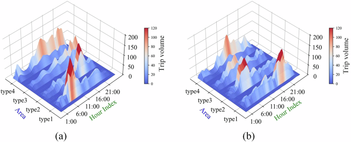
The temporal distribution of ride-hailing demand is analyzed in four typical regions, residential areas (Type 1), commercial CBDs (Type 2), scenic spots (Type 3), and entertainment areas (Type 4). Ride-hailing orders are concentrated during weekday mornings and evenings, as well as weekend afternoons and evenings. In large residential areas, the large travel demand is driven by commuting, as evidenced by huge departure flows between 7:00 and 9:00 and the arrival flows between 17:00 and 19:00. a Temporal distribution of ride-hailing departure demand, b Temporal distribution of ride-hailing arrival demand.
The Origin-destination (OD) distribution of ride-hailing orders exhibits distinct spatial characteristics in Fig. 3. Due to a large number of Beijing residents commuting from the suburbs to the city center for work on workdays and returning to the suburbs from the city center after work, the OD distribution is concentrated between the city center and the suburbs during the morning and evening peak hours in Fig. 3a, c. Additionally, as there are more entertainment and leisure trips during the evening rush hour, the number of trips in the city center is still higher. The volume of ride-hailing orders in the evening is higher than during off-peak hours in the daytime but lower than in rush hours, and the OD mobility patterns are mainly concentrated within the city center, with relatively shorter distances in Fig. 3d.
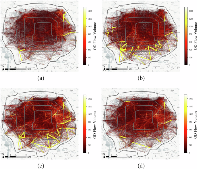
Due to a large number of residents commuting from the suburbs to the city center on weekdays and returning to the suburbs after work, high volume of OD pairs during peak hours in the morning, afternoon, and evening mainly concentrates between the city center and the suburbs. a ride-hailing orders from 7:00 to 9:00, b ride-hailing orders from 9:00 to 11:00, c ride-hailing orders from 17:00 to 19:00, d ride-hailing orders from 19:00 to 21:00.
The duration and distance characteristics of ride-hailing across different days of the week are shown in Fig. 4a, b and various periods during the day in Fig. 4c, d. To provide a more intuitive visualization of online ride-hailing service characteristics throughout the week, kernel density estimation plots are created to analyze the occupied and idle travel characteristics of ride-hailing mobility. Trip durations are primarily concentrated between 5 and 20 min, while trip distances are mainly concentrated within 10 km. In the early morning period of 0:00–6:00, the average idle time is slightly longer than in other periods in Beijing during workdays, while the average occupied time exceeds 20 min per order during morning and evening rush hours.
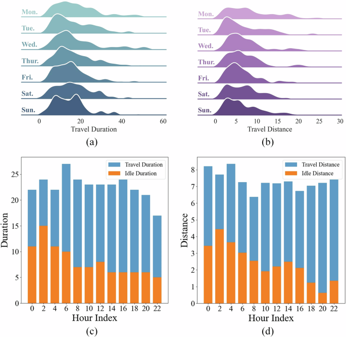
During the day of the week, trip durations are primarily concentrated between 5 to 20 min, while trip distances are mainly concentrated within 10 km. In the early hours of the morning, the average idle time is slightly longer than in other periods during workdays, while the average occupied time exceeds 20 min per order during morning and evening rush hours. a travel duration distribution, b travel distance distribution, (c) travel duration of occupied and idle vehicles per order, d travel distance of occupied and idle vehicles per order.
Arrival time prediction comparison
By leveraging extensive ride-hailing travel records, weather data, and POI data, our research investigates an explainable machine learning model Stacking-XCL to accurately estimate the arrival time. Stacking-XCL employs advanced tree-based models Extreme Gradient Boosting (XGBoost)38, CatBoost39, and Light Gradient Boosting Machine (LightGBM)40 algorithms, and further explains the inherent mechanism of arrival time prediction in ride-hailing services. We analyze the model performance for ride-hailing services in Beijing during both weekdays and weekends, encompassing peak and off-peak hours.
We introduce the measures used to evaluate the prediction errors and detail the results of benchmark models, including Least Absolute Shrinkage and Selection Operator (LASSO), Linear Regression (LR), Random Forest (RF), XGBoost, CatBoost, and LightGBM.Three evaluation metrics including Root mean square error (RMSE), Mean absolute error, Coefficient of determination (({R}^{2})) are assessed to compare the prediction performance of the models in Eqs. (1)–(3). ({y}_{i}) and ({hat{y}}_{i}) are the true and predicted travel times. (n) is the size of the test set.
Table 1 shows the prediction accuracy of the arrival time prediction models during weekdays and weekends. The XGBoost, CatBoost, and LightGBM algorithms are based on gradient-boosting decision trees, which perform significantly better than linear and RF models. Results verify that the stacking strategy combines the advantages of the three algorithms and outperforms any single base learner and all benchmark models on weekdays and weekends, as well as peak and off-peak hours scenarios. Specifically, on weekdays, the RMSE errors of the LR, RF, XGBoost, CatBoost, and LightGBM algorithms are 368.086, 462.350, 222.005, 236.101, and 240.826, and the corresponding ({R}^{2}) values achieve 0.6407, 0.4331, 0.8693, 0.8522, and 0.8462. The Stacking-XCL algorithm produces reliable results that accurately predict ride-hailing arrival time, where the RMSE error of the Stacking-XCL algorithm reduces to 221.255, and the ({R}^{2}) value improves to 0.8702. Besides, the Stacking-XCL model also shows advantages in predicting travel time during peak and off-peak hours. Figure 5 compares the prediction performance of different models on weekdays and weekends. The results indicate that the ensemble models such as XGBoost, CatBoost, and LightGBM exhibit good predictive accuracy, with predicted values closely aligned with the actual values. The Stacking-XCL model outperforms them by achieving smaller prediction errors, validating the superior performance in predicting arrival time on both weekdays and weekends.
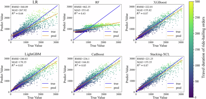
The Stacking-XCL model outperforms baseline models such as LR, RF, XGBoost, CatBoost, and LightGBM by achieving smaller prediction errors, validating the superior performance in predicting arrival time on both weekdays and weekends.
To further explain the inherent prediction mechanisms, the SHAP (SHapley Additive exPlanations) plot is used to interpret the black-box machine learning models.
Figure 6 provides an intuitive and global view of the impact of each feature on the arrival prediction results. Each row represents a specific feature, while the x-axis represents the SHAP value of the feature, indicating its impact on the model output. For each feature, the number of scatter points corresponds to the number of samples. The blue color represents lower feature values, whereas the red color represents higher feature values. The width of the scatter points reflects the abundance of sample data. The y-axis represents different features, sorted according to their importance. Among these factors, travel distance has the most significant impact on travel time prediction. As the distance increases, the corresponding SHAP value also increases, indicating a substantial positive effect of this feature on travel time prediction. Additionally, the departure time and the locations of the origin and destination have a notable influence on travel time prediction. Different departure times and locations affect the driver’s route choice behavior. During peak hours, drivers may take detours or alternate routes to avoid congestion on main roads. The subsequent influential factors are time-related variables, e.g., hour index, day index. Congestion levels on roads vary on time of day and day of week, resulting in fluctuations in travel time even for the same origin and destination. Besides, individual driver habits also have a certain impact on travel time prediction.
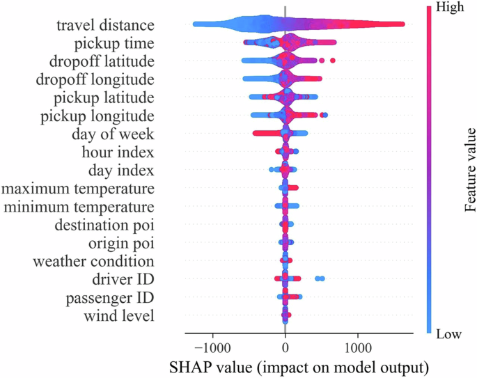
Positive SHAP values indicate that a feature contributes to increasing the prediction, while negative values suggest the opposite. Higher positive SHAP values indicate stronger positive influence, and higher negative values suggest stronger negative influence. The travel distance has the most significant impact on predicting travel time, followed by the departure time and the locations of the origin and destination.
Local interpretability refers to calculating the SHAP values of each feature for a specific sample, which can more clearly demonstrate how the model utilizes data features to make predictions for that sample. Figure 7 shows the impact of the main features on the predictions of three typical samples. By comparison, it is found that different features of different samples show different impacts, causing the predicted results to diverge towards different values while using the same base value as the reference. On the one hand, the same feature may have different effects on arrival time prediction. For example, a relatively low travel distance reduces the trip duration from the baseline value. When the travel distance is close to the average value, this feature presents almost no effect on the travel time prediction. On the other hand, the features have different impacts on the prediction for different samples. The divers’ travel behavior (diver ID) has an impact on the travel time predictions in Fig. 7a, b for the long-distance trips but has no significant impact in Fig. 7c, which speculates that when the trip duration is short, there is a decrease in the number of available routes, and the divers’ travel behavior shows less influence.
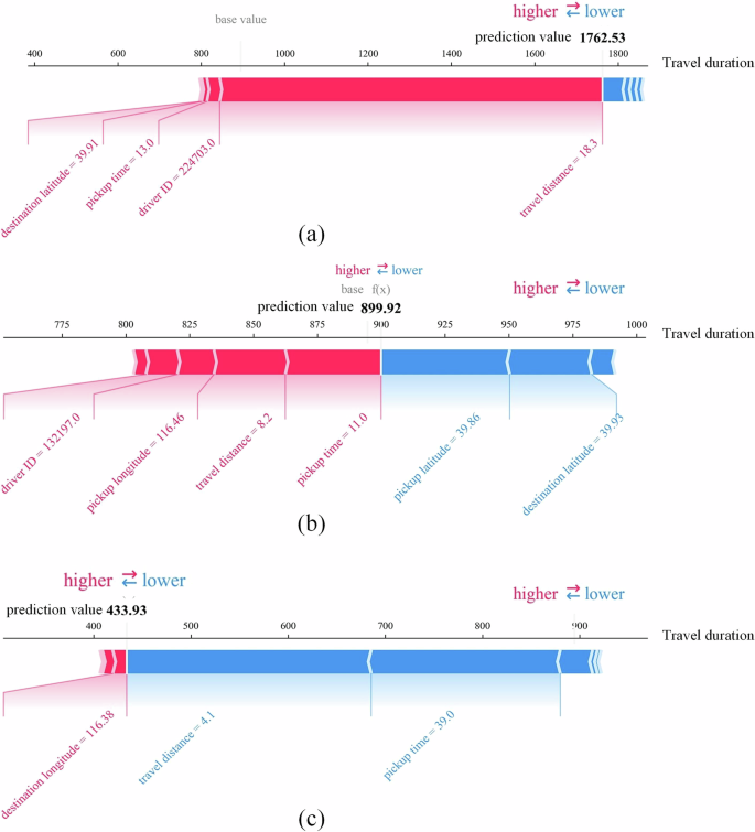
Local interpretability calculates the SHAP values of each feature for three typical samples. The red color indicates characteristics that lead to higher predicted values, while the blue color signifies characteristics that result in lower predicted values. Different samples exhibit varying impacts of different features, leading to divergent predicted results. a Local interpretability of long-distance ride-hailing trips, b Local interpretability of medium-distance ride-hailing trips, c Local interpretability of short-distance ride-hailing trips.
Result of optimizing order matching for carpooling
Carpooling services enable drivers with extra space in their vehicles to pick up passengers who have similar routes or destinations. We design an order-matching algorithm for the on-demand carpooling on the First-Arrive-First-Leave (FAFL) and First-Arrive-Last-Leave (FALL) scenarios. The trip-based shareability network is constructed based on the ride-hailing travel records. Since most vehicles used for carpooling are five-seat vehicles, for simplicity, this study assumes a vehicle capacity of five (including the driver and up to four passengers). With the proposed order matching model, a maximum allowable delay of 120 s and a maximum waiting time of 120 s are set for real-world ride-hailing orders. If matching constraints are satisfied, the potential carpooling orders are added to the candidate set for carpooling trips. We conduct the experiments with ride-hailing orders within every 5-min interval, evaluating the order matching performance with indicators such as number of orders after carpooling, time delay, saving time and distance, and passenger waiting time.
Table 2 shows the carpooling order matching results during peak hours on weekdays and weekends. The morning and evening peak order quantities on weekends appear at around 9:00 and 19:00, which is later than on weekdays at 8:00 and 17:00. The order-matching algorithm can effectively reduce the number of original orders, where the number of orders during peak hours on weekdays can be reduced by up to 34.18%, and on weekends can be reduced by up to 34.10%. Order matching exhibits greater potential during peak hours with high order densities and achieves more time and distance savings with lower delay and passenger waiting times. Specifically, during weekdays from 17:00 to 18:00, the average order delay for every 5 min is 6.65 s, and the additional waiting time for the second passenger is only increased by 27.44 s. Meanwhile, compared to not using the order-matching strategy where each order is served by one vehicle, the total trip duration with the order-matching strategy is saved by 841.56 s, and the travel distance is saved by 4223.36 m. During weekends from 17:00 to 18:00, the average delay every 5 min is 8.51 s, and the additional waiting time for the second passenger is increased by 38.36 s. When compared to not using the order-matching strategy, the time savings of the shared rides is 597.77 s, along with the travel distance saved by 3486.25 m. Figure 8 describes the dynamic carpooling result of the 5-min time granularity during the whole day. The order-matching strategy for carpooling slightly increases the waiting time for the second passenger but has significant effects on the saving of travel time and distance. Therefore, carpooling can reduce the original number of ride-hailing orders while ensuring passenger service quality, and improving the operational efficiency of ride-hailing services.
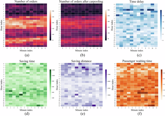
Real-world ride-hailing orders are used to evaluate the order matching performance with indicators on (a) number of orders, (b) number of orders after carpooling, (c) time delay, (d) saving time, (e) saving distance, (f) passenger waiting time. Time delay refers to the difference between the expected arrival time at the destination with carpooling and the actual arrival time. Saving time and distance signifies the time and distance saved through carpooling. Carpooling may slightly increase the waiting time for the second passenger compared to the actual pick-up time.
Emissions reductions with carpooling and vehicle dispatching
The vehicle dispatching in ride-hailing services can be described as assigning a series of vehicles to meet the dynamic travel demands of passengers. The Hopcroft-Karp algorithm is applied to assign vehicles to serve passengers and reposition, allowing drivers to efficiently serve multiple orders. The carbon emissions before and after carpooling are quantified using the COPERT III model, considering the influence of vehicle speed on different types of pollutants. This approach considers traffic congestion during different periods and calculates the actual speed of vehicles from the ride-hailing orders, resulting in a more precise estimation of pollutant emissions.
The result of optimizing vehicle dispatching on peak hours of weekdays is presented in Table 3. The trips with carpooling comprise the successfully matched carpooling orders and the original left orders that remain unmatched. Hourly statistics reveal that the number of orders is 2606, 1879, and 1903 between 7:00, 8:00, and 9:00, respectively. By implementing the order-matching strategy, the number of orders for carpooling decreases to 1915, 1453, and 1423. When performing the vehicle dispatching with the original orders between 7:00 and 8:00, 2606 orders require the service of 1006 vehicles to meet passengers’ travel demand, resulting in a total travel distance amounting to 11461.21 km. The COPERT III model is adopted to calculate the pollutant emissions with the actual driving speeds of different ridesharing vehicles. The analysis reveals that in one hour, all vehicles collectively consume 1129.11 kg of fuel consumption, emitting 6068.94 g of CO, 329.56 g of HC, 995.28 g of NOx, 3590.57 kg of CO2, and 33.87 g of PM2.5. With the order-matching strategy, the number of pooling orders decreases to 1915, requiring only 684 vehicles to fulfill the travel demand. As a result, the total distance traveled by vehicles is reduced by 25.17% to 8576.18 km. The pollutants emissions show a decline, where CO, HC, and NOx amount to 4437.94 g, 234.33 g, and 742.87 g, respectively. The total fuel consumption of these vehicles decreases to 805.69 kg, leading to reduced emissions of CO2 and PM2.5 as 2562.10 kg and 24.17 g with a reduction of 28.64%.
During the evening peak period, passenger travel demands are not as concentrated as during the morning peak hours, and a high volume of travel orders persists until nighttime. Between 19:00 and 20:00, the ride-hailing demand within the Beijing Third Ring Road area amounts to 1618 trips, requiring 559 vehicles to fulfill these orders, with a total vehicle distance of 7778.48 km. After matching similar orders through carpooling, the number of orders decreases to 1221, requiring 406 vehicles to serve them, resulting in a total vehicle distance of 6179.84 km. The reduction in the number of vehicles and total distance traveled is 27.37% and 20.55%. The decrease in serving orders results in reduced pollutant emissions. With the carpooling strategy, the emissions of NOx and CO2 from vehicles amount to 525.55 g and 1658.69 kg, compared to 665.37 g and 2167.23 kg without implementing the order-matching strategy, demonstrating reductions of 21.01% and 23.47%.
Figure 9 provides an overview of the changes in the travel speed and pollutant emission distribution. Ride-hailing vehicles exhibit relatively higher speeds during the time slots of 6:00 to 8:00 and 10:00 to 12:00, reaching a maximum speed of ~78 km/h in Fig. 9a. However, during the morning peak hours from 8:00 to 10:00, the vehicles experience slower speeds, with an average speed of only 19.72 km/h. Throughout the daytime period, traffic congestion caused by a high volume of vehicles within the Beijing Third Ring Road limits the speed of ride-hailing vehicles not exceeding 25 km/h. In Fig. 9b, results demonstrate that a speed of ~60 km/h emerges as the optimal balance, minimizing fuel consumption and effectively reducing pollutant emissions, such as CO (Carbonic Oxide), HC (Hydrocarbons), NOx (Nitrous Oxides). Besides, it is crucial to avoid driving speeds below 20 km/h as they generate more fuel consumption and various types of pollutants.
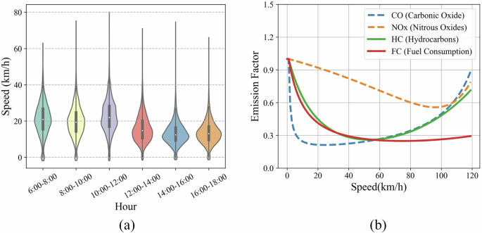
Due to traffic congestion, ride-hailing vehicles experience variations in their driving speeds throughout the day. A speed of ~60 km/h is considered the optimal balance point, as it allows for maximum reduction in fuel consumption while effectively minimizing pollutant emissions. a Real-time travel speed distribution, b Emission factor changes with different travel speeds.
Discussion
The ride-hailing service provides fast, convenient, and flexible transportation options while promoting efficient resource utilization and sustainability. Carpooling is an emerging travel mode where multiple individuals traveling in the same direction share a single vehicle, optimizing vehicle occupancy without increasing the number of vehicles or altering road structures. This study utilizes large-scale ride-hailing travel records data and proposes a dynamic vehicle dispatching framework based on arrival time prediction and carpooling. Results indicate that accurate estimation of arrival time can significantly enhance the level of carpooling in ride-hailing services. By implementing efficient order-matching strategies, not only can passenger service efficiency be improved, and detour distances minimized, but it also leads to a substantial reduction in fleet size and a decrease in pollutant emissions.
First, the spatio-temporal characteristics of ridesourcing mobility are analyzed utilizing large-scale travel order data. The travel patterns of ridesourcing services exhibit distinctions between weekends and weekdays, primarily concentrated during weekday rush hours in the morning and evening, as well as during weekend afternoons and evenings. Trip durations are primarily concentrated between 5 and 20 min, while trip distances are mainly concentrated within 10 km in Fig. 4a, b. The idle distance and time are significant influencing factors for carbon emissions estimation. Shorter idle trips indicate higher utilization efficiency of online ride-hailing services, while longer idle distances and time increase carbon emissions. During the peak period, the idle distance is shortened due to the high density of trip orders, but the travel time does not decrease significantly due to the possible traffic congestion. The idle distance and time of online ride-hailing services on workdays reach up to 58% and 62% of the occupied distance and time Fig. 4c, d, with an average of 33% and 36%. These high proportions of idle distance and time suggest that there are still efforts to improve the utilization efficiency of online ride-hailing services and reduce pollutant emissions.
Second, accurate arrival time prediction facilitates efficient passenger matching for carpooling purposes. This study investigates an explainable machine learning model to accurately estimate the arrival time, using a hierarchical framework that combines multiple algorithms constructed for travel time prediction in ride-hailing services. Experimental results conducted on two consecutive months of ride-hailing order data in Beijing demonstrate that the proposed explainable machine learning models, which consider spatio-temporal features of pickup and drop-off locations as well as external environmental factors, not only accurately predict vehicle arrival times with average accuracy exceeding 87% in different scenarios, but also provides detailed explanations for the prediction results. Figure 5 compares the prediction performance of different models on weekdays and weekends. The results indicate that the ensemble models such as XgBoost, CatBoost, and LightGBM exhibit high predictive accuracy, with predicted values closely aligned with the actual values. The Stacking-XCL model outperforms them by achieving smaller prediction errors, validating the superior performance in predicting arrival time on both weekdays and weekends. Precise estimation of arrival time allows ride-hailing platforms to optimize the potential order matching and vehicle dispatching process, ensuring that individuals are grouped in the most time-efficient manner. As a result, waiting times for passengers are reduced, and the utilization of vehicle capacity becomes more effective.
Machine learning interpretability provides insights and understanding into how models make predictions. The SHAP value offers a method to elucidate the contribution of each feature in the model’s predictions, which provides insights into the most significant features and how to affect the predictions. Global and local interpretability for the travel duration prediction model is depicted in Figs. 6 and 7. The travel distance of the trip has the greatest influenceon predicting travel time tasks, followed by the departure time and locations. The estimation of travel time is affected by the trips on weekdays or weekends, during peak hours or off-peak hours. In addition, the POI features around the origin and destination locations reflect the land use characteristics, and the location features where passengers pick-up and drop-off also affect the estimation of travel time. The wind speed affects slightly on travel time prediction tasks, as ride-hailing services offer a comfortable riding experience and are less affected by weather conditions compared to other modes of transportation such as shared bikes and public transportation. It is noteworthy that the impacts of different features in the model are consistent with the real situation, which demonstrates that the SHAP method is effective in interpreting the machine learning models and identifying the key factors that influence the prediction results.
Third, to make each carpooling trip more efficient and eco-friendly, we build a trip-based shareability network for on-demand carpooling to identify potential matching orders with similar origins and destinations. Two carpooling trip modes, FAFL and FALL are designed to reduce the vehicle fleet size, time delay, and waiting time of passengers. The order-matching result for carpooling is depicted in Fig. 8. Figure 8a describes the original volume of ride-hailing orders, and Fig. 8b shows the order volume after carpooling. It can be observed that the proposed order-matching strategy significantly reduces the order volume and is effective in various time periods. The order-matching strategy fully explores and utilizes the potential carpooling opportunities during peak hours when the order volume is high. Figure 8c is the delay distribution with order matching, and most of the delays caused by order matching are at a relatively low level, with minimal impact on the timeliness of the orders. However, during the early morning hours when the order volume is low, matching orders that are distributed far apart cause relatively serious delays. Figure 8d, e explore the time and distance savings after order matching. During morning peak hours, due to road congestion, there are cases where distance savings are greater with the order-matching strategy while the time-saving proportions are relatively low. Figure 8f depicts the extra waiting time for passengers after order matching, and it can be observed that the waiting time is relatively low, mostly around 30 s, with the highest waiting time not exceeding 1 min. Compared with the trip duration and distance savings achieved by carpooling, the extra waiting time is within an acceptable level.
Furthermore, leveraging the predicted ride-hailing arrival times and order-matching results, a graph-based algorithm is designed for vehicle dispatching with high computing performance. The COPERT III model is adopted to calculate the pollutant emissions with the actual driving speeds of different ridesharing vehicles. In comparison to the current operations, a reduction of 25.25% in fleet size and a simultaneous decrease of 21.65% in pollutant emissions are achieved in Table 3. The results demonstrate that potential order matching and vehicle dispatching processes lead to a slight increase in passenger waiting time while enhancing the operational efficiency of ride-hailing services and reducing pollutant emissions. Figure 9 demonstrates the influence of real-time driving speeds on fuel consumption and emission factors. Notably, vehicle speed has a significant impact on carbon emissions, resulting in noticeable variations in pollutant emissions across different speed intervals. A speed of ~60 km/h emerges as the optimal balance, minimizing fuel consumption and effectively reducing pollutant emissions. Conversely, it is crucial to avoid driving speeds below 20 km/h as they generate more of all types of pollutants. While most taxi drivers strive to maintain speeds at a high fuel efficiency level whenever feasible, the actual driving conditions, such as road conditions and traffic congestion, often force vehicles to operate at lower speeds, leading to substantial pollutant emissions. Encouraging carpooling initiatives can positively contribute to reducing traffic congestion, improving traffic speeds, and further enhancing energy-saving and emission-reduction efforts.
Methods
Arrival time prediction model
Emerging explainable machine learning algorithms are designed to provide more transparent and interpretable results, allowing operators to understand how the algorithm arrived at its predictions or decisions. These algorithms extract effective features from vast amounts of raw data, and dynamically adjust parameters during the training process, which enables accurate and stable results of various prediction tasks. XGBoost (eXtreme Gradient Boosting) is an ensemble learning algorithm based on decision trees that has found widespread application in prediction tasks38,41. XGBoost uses the gradient boosting framework to optimize models, continuously training weak classifiers to improve the overall accuracy of the model, with each weak classifier being a decision tree. XGBoost parallelizes the sequential process of generating trees with distributed computing, making it capable of processing massive amounts of data in a short time42.
CatBoost stands as a machine learning algorithm that builds upon Gradient Boosting Decision Tree (GBDT). CatBoost supports both categorical and numerical features, and can automatically detect which features are categorical and process them appropriately. During the training process, CatBoost builds an independent subtree for each category and then merges these subtrees into the final decision tree. This approach effectively solves the problem of categorical features and improves the accuracy of the model43. CatBoost constructs balanced trees with symmetric structures. In each step, the feature-split pair that yields the lowest loss is selected and applied to all nodes at that level. This method achieves reduced training time, fast model application, and avoids overfitting that occurs when multiple datasets are arranged directly39.
LightGBM, short for light gradient-boosting machine, is an improved version of the GBDT algorithm. It linearly combines multiple weak regression trees into a powerful regression tree, using the histogram decision tree optimization algorithm to reduce time complexity40. The basic principle of LightGBM is to iteratively fit the decision tree model and optimize the loss function through gradient descent. LightGBM introduces Gradient-based One-Side Sampling and Exclusive Feature Bundling to optimize the training process. The computational complexity and accuracy of the model are controlled by adjusting hyperparameters, such as the learning rate, number of leaf nodes, and maximum depth44.
Stacking is a hierarchical model integration framework that combines and fuses the prediction information of multiple algorithm models to achieve superior performance over single algorithms while maintaining good generalization ability45. This study investigates an explainable machine learning model using a hierarchical framework that combines multiple algorithms constructed for travel time prediction in ride-hailing services in Fig. 10 The origin dataset is formed by combining ride-hailing orders, weather conditions, and POI features of both the origin and destination. The ride-hailing data encompasses key attributes such as pickup and drop-off times and locations. The XGBoost, CatBoost, and LightGBM are employed as base models, and a Linear Regression as the meta-learner to construct the Stacking-XCL model. To prevent overfitting, the Stacking-XCL model applies K-fold cross-validation during the training of the base models. The training data are divided into ({K}) subsets, with one subset used for testing and the remaining subsets used for training all base models. Afterward, all prediction results are combined to form the training data for the meta-model. The green squares in Fig. 10 represent the predictions of the validation subset from the (K) training iterations of the base models. In this way, the higher-level meta-learner utilizes the strengths of the base models to produce the final prediction output. The Stacking algorithm has the advantage of integrating the strengths of multiple base models, thereby producing more accurate and robust prediction results46.
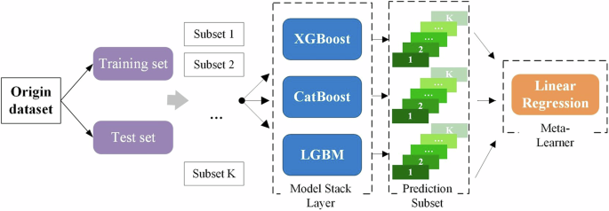
The XGBoost, CatBoost, and LightGBM are employed as base models, and a Linear Regression as the meta-learner to construct the Stacking-XCL model. The Stacking-XCL model applies K-fold cross-validation during the training of the base models. The training data is divided into K subsets, with one subset used for testing and the remaining subsets used for training all base models. Afterward, all prediction results are combined to form the training data for the meta-model. In this way, the higher-level meta-learner utilizes the strengths of the base models to produce the final prediction output.
Deep neural networks and other conventional machine learning models are frequently characterized as “black boxes” because it is difficult to interpret and understand their internal working process. Explainable machine learning aims to overcome this limitation by designing models that are transparent and can provide human-understandable explanations for result predictions and decisions38. SHAP (Shapley Additive Explanations) is a method for interpreting machine learning models that are based on the concept of Shapley values in game theory. It is used to explain the impact of each feature on the prediction results for each sample by assigning relative importance to input features47,48,49. When explaining the prediction of a sample, Shapley values consider all possible combinations of each feature and calculate its contribution to the prediction result. A positive Shapley value represents a positive effect of the feature on the model prediction, while a negative value represents a negative effect. The Shapley value is calculated by adding one feature after another to the model and comparing the output of the model with and without that feature. Therefore, for a specific feature (n) and input data (x), the Shapley value ({varPhi }_{n}left(f,xright)) can be calculated using Eq. 4.
In this context, (f) is the established machine learning model and (N) is the set composed of all the features. (S) is a subset of features that have already been added to the model, and (fleft(Sright)) is the prediction result obtained using this subset (S). Since the prediction may depend on the order in which features are added, the contributions of all possible feature combinations are averaged using a ranking function. The SHAP package is adopted for computing efficiency, where the feature importance is then calculated by summing the magnitude of the SHAP values for all feature samples. SHAP values can evaluate not only the global importance of features, but also provide specific interpretability for each sample locally. This offers a more accurate and transparent explainability of the “black boxes” models, which is crucial for helping decision-makers understand the results50,51.
Potential order matching for carpooling
The ride-hailing services have encountered problems such as long empty driving distances during off-peak hours, passenger shortages due to its operation, insufficient vehicle availability, and traffic congestion. To address these issues, better organizing ride-hailing services fully utilize the vehicle space resources and effectively improve the supply level of the ride-hailing market, without increasing the supply of vehicles or changing the existing road conditions. The emerging carpooling service allows drivers with extra space in their vehicles to pick up fellow passengers who share similar routes or destinations. Shared ride services can lead to savings in both travel distance and travel time for the ride-hailing vehicles in the system by serving two orders simultaneously. The effective order-matching strategy enhances the seating utilization of vehicles, while dynamic vehicle dispatching aims to improve the overall utilization of ride-hailing vehicles, thereby reducing their idle travel distance and carbon emissions52.
When traveling with ride-hailing services, passengers send travel requests to the platform. Each demand ({r}_{i}in R) is defined as a tuple ({{o}_{i},,{d}_{i},{t}_{i}^{p},{t}_{i}^{d}}), representing pick-up and drop-off locations, and expected pick-up and drop-off time, respectively. (R) is the order pool dynamically collected by the system over a period of time, e.g., a few minutes. Based on the submitted travel requests, the platform gathers the passenger’s desired pickup and drop-off locations, along with their expected departure time. Once multiple travel requests are collected within a specific period, potential orders are matched with the proposed algorithm. To simplify the matching process between drivers and passengers, the pick-up and drop-off locations are assumed to be aligned with the nearest intersection. In this study, a trip-based shareability network is constructed to address the order-matching problem for carpooling5. A trip is represented as a single node with four attributes: pick-up location, drop-off location, departure time, and arrival time. The connection between two nodes is determined by the spatial and temporal characteristics of the two trips. A maximum weight graph-matching algorithm is used to determine the matching orders, where the edge between nodes indicates that the two orders are matched. The objective of the graph-matching algorithm is to maximize the number of potential carpooling orders under the current situation.
This paper considers the matching of two orders, as 90.50% of carpooling trips only involve two shared orders, and matching three or more shared orders increases trip uncertainty, making it more likely that passengers’ trips be delayed7. For example, the DiDi transportation platform strictly controls detours, and ride-hailing companies only allow drivers to accept two carpooling orders at the same time. When one of the orders ends, the driver can accept other carpooling orders. Figure 11 shows the two different matching modes when potential carpooling orders are matched, where ({O}_{i}) represents the departure location of order (i), and ({D}_{i}) represents the arrival location of order (i). ({O}_{i}^{{prime} }) and ({D}_{i}^{{prime} }) are the actual departure and arrival locations in the matching trips, and ({t}_{i}^{p}) and ({t}_{j}^{p}) represent the expected departure times of orders (i) and(,j). (delta) is the time window constraint. To reduce the waiting time for users after placing an order, only orders within the time window will be matched. Δ is the allowable delay of passengers, and a carpooling order is feasible only when the departure and arrival times of both passengers are within their allowable delays. The notations in the carpooling order-matching model are listed in Table 4.
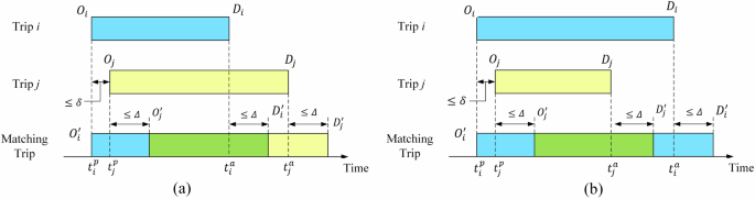
a First-Arrive-First-Leave (FAFL), b First-Arrive-Last-Leave (FALL). In FAFL carpooling mode, when two orders meet the carpooling constraints, the vehicle will pick up the first passenger at the departure location ({O}_{i}) and pick up another passenger at the departure location ({O}_{j}). Then, the vehicle will arrive at the destination ({D}_{i}) to drop off the first passenger and subsequently arrive at the destination ({D}_{j}) to drop off the other passenger. In the FALL carpooling mode, the vehicle picks up the first passenger at the starting location ({O}_{i}) and then pick up another passenger at the starting location ({O}_{j}). The vehicle will first arrive at the destination ({D}_{j}) and then arrive at the destination ({D}_{i}) to drop off the passengers.
Figure 11a shows the FAFL carpooling mode, when two orders meet the carpooling constraints, the vehicle will pick up the first passenger at the departure location ({O}_{i}) and then pick up another passenger at the departure location ({O}_{j}). Then, the vehicle will arrive at the destination ({D}_{i}) to drop off the first passenger and subsequently arrive at the destination ({D}_{j}) to drop off the other passenger. Order ({i}) is the first order in the carpooling service, and therefore its expected boarding time is the same as the actual boarding time. The expected boarding time of order ({j}) is later than the actual boarding time due to the impact of the carpooling process. Equation (5) specifies that the expected pick-up time of two carpooling orders should not exceed the time window constraint. In Eq. (6), the vehicle is allowed to arrive at the second passenger’s pick-up location before their scheduled pickup time. However, the vehicle must not arrive later than the latest expected departure time, which is calculated as the expected pickup time ({t}_{j}^{p}) plus the passenger’s allowable delay (varDelta). Equations (7) and (8) indicate that the vehicle must arrive at the drop-off locations of the first and second passengers no later than the latest arrival time.
Figure 11b is the FALL matching mode. The vehicle picks up the first passenger at the starting location ({O}_{i}) and then pick up another passenger at the starting location ({O}_{j}). The vehicle will first arrive at the destination ({D}_{j}) and then arrive at the destination ({D}_{i}) to drop off the passengers. ({r}_{i}) and ({r}_{j}) are the two carpooling orders. To account for the vehicle operating characteristics in this scenario, Eqs. (7) and (8) should be replaced with Eqs. (9) and (10).
By setting time window constraints (delta) and (varDelta) based on constraints (5)–(10), the algorithm can effectively filter potential carpooling orders. According to the FAFL and FALL carpooling modes, satisfying either mode can be qualified as a potential carpooling order and added to the candidate set. Taking the FAFL matching mode as an example, ({t}_{i}^{a}) is the expected arrival time of the trip (i) and ({t}_{i}^{{a}^{{prime} }}) is the actual arrival time of the trip (i). The actual arrival time ({t}_{i}^{{a}^{{prime} }}) is calculated with the departure time of the trip (i), the travel time between ({O}_{i}) and ({O}_{j}), and the travel time between ({O}_{j}) and ({D}_{i}) in Eq. (11). The actual arrival time of the trip (j) is calculated in Eq. (12). The time delay ({T}_{S}^{{delay}}) refers to the discrepancy between the actual arrival time at the destination of two trips and the expected arrival time due to the matching order (S) in Eq. (13). ({T}_{S}^{{saving}}) signifies the time saved through shared rides, computed as the summation of the travel duration for each trip minus the total travel time with the sharing process in Eq. (14). ({D}_{S}^{{saving}}) is the travel distance reduction with carpooling, which can be calculated accordingly with Eq. (15). ({T}_{S}^{{waiting}}) is the waiting time of the second passenger compared to the actual pick-up time in Eq. (16). To match the orders with different objectives, a maximum-weight matching algorithm is employed on the graph structure to obtain the order-matching results.
Vehicle dispatching and carbon emission estimation
Vehicle dispatching in ride-hailing services can be described as dispatching a series of vehicles to meet the travel demands of users within a certain period. This can be regarded as a maximum matching problem between vehicles and a series of trip orders on a bipartite graph, which is to find the minimum vehicle fleet size under different constraints and objectives to fulfill the users’ travel demands. The Hopcroft–Karp algorithm is an efficient algorithm used to solve the maximum matching problem in a bipartite graph, which is an improvement over the Hungarian algorithm6. In the constructed trip-based graph, the nodes in the network represent a trip, and each edge denotes the vehicle routes to serve continuous trips. The Hopcroft–Karp algorithm works by finding augmenting paths in the bipartite graph. Sequences of edges that alternate between being in and out of the matching, such that swapping which edges of the path are in and which are out of the matching produces a larger matching. The key insight of the Hopcroft–Karp algorithm is that the maximum cardinality matching can be found by repeatedly finding augmenting paths until no more augmenting paths exist. The time complexity of the Hopcroft–Karp algorithm is ({rm{O}}(sqrt{V}* E)), where (V) and (E) represent the number of vertices and edges in the graph.
The COPERT III model is a widely used model for estimating traffic emissions, which can accurately estimate and predict transportation emissions based on factors such as vehicle characteristics, driving speed, travel mode, and road characteristics. The emission model covers different types of vehicles, including cars, buses, trucks, and public transport, together with different types of fuels and pollutants, such as COx, NOx, et al.53,54. Based on a large amount of reliable experimental data, the model is compatible with various parameter variables and different standards. The COPERT III model divides traffic emissions into three categories: hot-start emissions, cold-start emissions, and evaporative emissions. Among these, hot-start emissions are the main focus as they are the primary engine emissions during normal driving conditions15. Cold-start emissions refer to the emissions produced by the engine operation, while evaporative emissions arise from fueling and temperature changes. Cold-start emissions and evaporative emissions pay less significance in terms of overall emissions. The hot emission factor (({{EF}}_{eta })) is a crucial parameter in the COPERT III model, representing the total amount of a specific pollutant(,eta) emitted by a single vehicle per kilometer traveled (in (g/{km})). It is calculated based on the vehicle’s driving speed (in ({km}/h)) and described by a mathematical function with five parameters: (a,{b},{c},{d},) and ({e}) in Eq. (17).
Table 5 presents the pollutant emission factors of the COPERT III model. CO2 and PM2.5 have global effects on climate change and can be computed using Eqs. (18) and (19).
For each ride-hailing vehicle (k), assuming that there are no return trips after completing the last ride, the total amount of a specific pollutant (eta) generated from completing all (N) rides can be calculated by the sum of the pollutant emissions from three parts in Eq. (20).
Where ({E}_{eta }^{k}) represents the total amount of pollutant (eta) emitted by a ride-hailing vehicle (k) while completing all (N) rides. ({E}_{1}) is the emission from the starting point to the first-served ride, where (E{F}_{eta }^{k,0}) represents the hot emission factor for pollutant (eta) during this process, and ({l}_{eta }^{k,0}) is the distance between the two locations. ({E}_{2}) is the sum of emissions for serving rides from the pick-up location to the drop-off location. ({E}_{3}) is the sum of emissions between two consecutive trips, and ({l}_{eta }^{k,m}) represents the distance from the drop-off location of trip (m) to the pick-up location of the trip (m+1).


Responses