Scalability challenges of machine learning models for estimating walking and cycling volumes in large networks

Interest in active transportation planning and policymaking continues to grow due to its recognized health, environmental, and economic advantages. Active transportation is increasingly viewed as a sustainable solution to urban mobility challenges, promoting healthier populations and reducing environmental impacts. However, the absence of robust active transportation data has hindered the ability to make well-informed decisions regarding infrastructure investment and policy development. While crowdsourced data like Strava and mobile phone data have shown promise in capturing cycling and walking patterns^{1,2,3,4,5,6,7,8,9}, concerns persist regarding their scalability and reliability, particularly for large-scale applications.

Prior research has attempted to address biases and limitations inherent in these data sources^10,11,12, often focusing on localized contexts and predominantly on cycling behavior. However, the challenges associated with upscaling these methodologies to cover large-scale networks have received limited attention. This study seeks to bridge this gap by developing a comprehensive machine learning-based approach tailored specifically for large-scale implementation. Covering all phases of model development, including training, testing, and inference, the research aims to estimate link-level walking and cycling volumes across the extensive New South Wales (NSW) Six Cities Region in Australia with 188,999 walking links and 114,885 cycling links.

Crowdsourced data such as Strava can capture cycling patterns, but they have been shown to be biased towards specific types of travelers^13,14,15,16. Mobile phone data can also capture active travel patterns, but the sample representativeness and the quality of the data, especially for short trips such as walking and cycling, have been subjects of debate^{17,18,19,20,21,22,23}. A growing number of studies have proposed methods to correct the sampling bias and inaccuracies in crowdsourced and mobile phone data in the context of active transportation planning^10,11,12. Integrating the emerging crowdsourced and mobile phone data with other data sources have been proven to estimate more representative active mobility patterns.

Crowdsourced data often lack the quality assurance of traditional geographic data collection measures. Jestico et al.¹⁰ raised concerns around potential biases from user submitted content that are difficult to quantify without comparing against reference data sources. They analyzed Strava cycling data in the Vancouver, BC, Canada area and found that the average Strava sampling to population ratio is 1:51 with significant variation across different sites ranging from 10% error to 100% error. In a follow up study, Roy et al.¹⁴ argued that crowdsourced cycling data are biased as they oversample recreational riders. However, they demonstrated that different geographical variables can be quantified to correct the bias in crowdsourced data. They trained a model using observed cycling counts from 44 locations across the Maricopa Association of Governments (MAG), Arizona, USA. They demonstrated that the proposed modeling approach is broadly applicable for correcting bias in crowdsourced active transportation data when official observed counts and geographical data are available. In a more recent study, Nelson et al.¹² also argued that to overcome the bias in crowdsourced data, statistical models can be developed to estimate total cycling volumes by integrating Strava data with official observed counts and a range of geographic data. They developed and tested the modeling approach in five different cities across North America including Boulder (CO), Ottawa (ON), Phoenix (AZ), San Francisco (CA), and Victoria (BC).

Despite the growing literature on the use of crowdsourced and mobile phone data sources^{1,2,3,4,5,6,7,8,9} and different modeling methodologies to overcome the bias in the data, most previous studies focused on cycling only and demonstrated the applicability of the modeling approach in relatively small-scale networks and were limited to use of observed count data from small number of locations.

Building upon existing literature, our methodology extends beyond cycling to include walking, demonstrating its adaptability and robustness on a large-scale regional level. The study makes several key contributions. First, it highlights the limitations of using observed walking and cycling count data from limited and geographically biased locations. To address this, we propose a new spatial and temporal cross-validation approach that improves model training and testing robustness and performance. Additionally, the study identifies common data gaps in Strava and mobile phone-based data, such as missing links with low activity. Our machine learning-based modeling approach integrates crowdsourced and mobile phone data with a diverse array of population, land use, and other datasets. This holistic methodology provides an in-depth understanding of the challenges and limitations inherent in all phases of model development—from training and testing to inference—considering the large-scale extent of the study networks and the relative scarcity of observed pedestrian and cycling count data. Furthermore, we propose a technique to identify and mitigate model estimate outliers, ensuring the accuracy and reliability of large-scale inference applications. Moreover, by extending the methodology beyond cycling to include walking, a less explored active transportation mode, the study demonstrates its applicability and validity for a broader range of active transportation planning needs. These contributions collectively enhance the planning and policies supporting sustainable forms of transportation at a regional scale using advanced data-driven methodologies.

The research outcomes align with the Sustainable Development Goal 11 (SDG 11), which focuses on making cities and human settlements inclusive, safe, resilient, and sustainable. It particularly supports efforts to improve transportation systems to make them more sustainable and to enhance inclusive urbanization by promoting safe and accessible transportation options like walking and cycling.

The NSW Six Cites Region encompasses six cities in the state of NSW, Australia including Lower Hunter and Greater Newcastle, Central Coast, Illawarra-Shoalhaven, Western Parkland, Central River, and Eastern Harbour. The region encompasses 43 local government areas with a total area of over 2.25 million hectares and population of 6.27 million residents (2021).

The walking network of the study area is constructed using the Geoscape PSMA network²⁴ including a total of 188,999 links. The cycling network is constructed using OpenStreetMap and Transport for NSW Bicycle Infrastructure Network data²⁵ including a total of 114,885 links. Note that links here represent streets in the network. See Fig. 1. Our estimates suggest that a total of 7.1 million walking trips occur per weekday and 6.7 million walking trips occur per weekend across the entire study region. We also estimate a total of 260,000 cycling trips per weekday and 406,000 cycling trips per weekend in the entire NSW Six Cities Region. This highlights the extensive and comprehensive nature of the presented modeling approach tailored for large-scale implementation. The geographical extent of the two networks introduces unique modeling challenges related to all three aspects of model training, testing, and inference that are discussed later in the manuscript in details and shape the main contributions of this study.

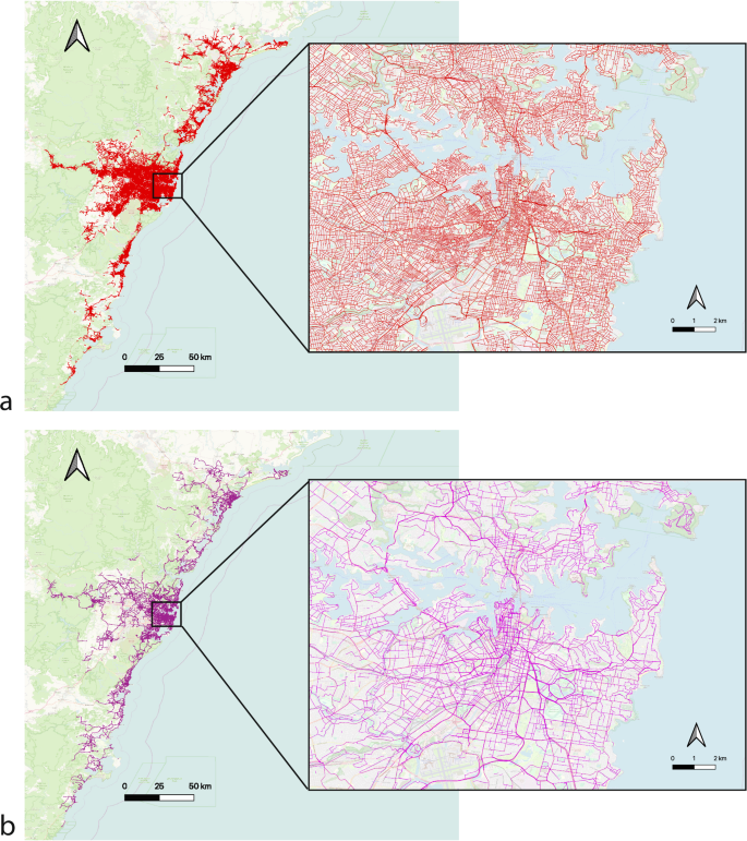
a Walking network with 188,999 links and b cycling network with 114,885 links in the NSW Six Cities Region, Australia.

Full size image

To better understand the error in the original mobile phone and crowdsourced data, we first assess both the mobile phone-based and Strava data’s ability to directly explain observed walking and cycling volumes. Figure 2a, b shows the relationship between link-level mobile phone-based walking counts vs. observed walking counts across all sites in the study area, as well as the relationship between link-level Strava cycling counts vs. observed cycling counts. Significant underestimation is observed across both data sources compared to the observed counts. Table 1 provides a summary of the performance of the two data sources against official observed walking and cycling counts including three main measures of R², Mean Absolute Error (MAE) and Root Mean Square Error (RMSE). Note that the unit of MAE and RMSE is the same as the original count data. The analysis results confirm the presence of significant bias and under-representation issues in crowdsourced and mobile phone data.

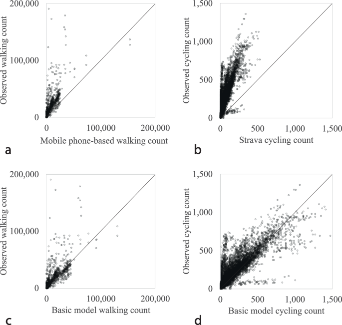
a Relationship between the mobile phone-based walking counts and observed walking counts, and b Relationship between Strava cycling counts and observed cycling counts across all sites in the study area. Base (naïve) c walking model and d cycling model count estimates against observed walking and cycling counts.

Full size image

Next, we build the naïve or base models. Using the mobile phone-based walking count data as the sole predictor, an ordinary least squares (OLS) regression is estimated. We also estimate a similar OLS regression model using Strava cycling count data as the sole predictor. See Table 2 for the estimated coefficients and the models’ performance metrics. Figure 2c, d illustrates the estimated walking and cycling counts against the observed counts when the base models are used. Results suggest that on average, every single Strava bicycle trip in the study area represents 3.14 total cycling trips while for the mobile phone-based walking data every single counted pedestrian trip represents 1.78 total pedestrian trips. While the naïve models’ performance exhibit significant improvement compared with the original crowdsourced and mobile phone data, the following sections of the manuscript demonstrate the extent that the models’ performance can further improve with extensive machine learning training and testing, and when integrated with other data sources.

Here, we comparatively examine, train, and test several statistical, machine learning and ensemble learning models, following the overall methodology proposed by Nelson et al.¹². To assess both the walking and cycling models’ goodness of fit, we use three main measures of R², MAE and RMSE computed on both the training and testing data set as shown in Tables 3 and 4. Figure 3 also provides a comparative illustration of the predictive power of a set of the developed walking and cycling models.

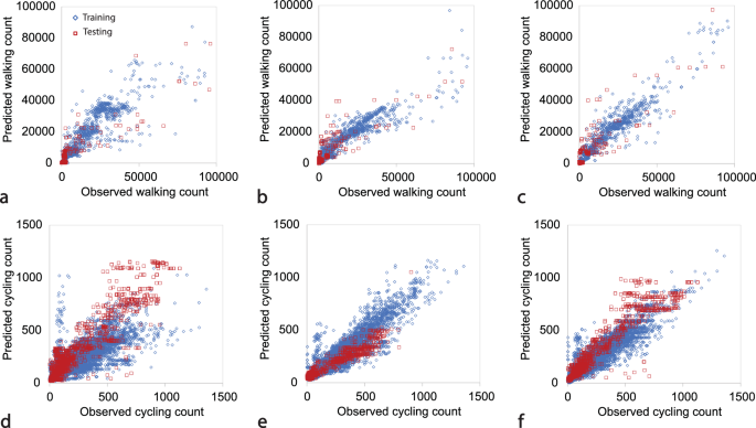
Walking models: a Stacking Regression, b Voting Regression, and c Gradient Boosting Regression; and cycling models: d Stacking Regression, e Voting Regression, and f Gradient Boosting Regression. Y axis represents the model predictions and X axis represents the observed walking or cycling counts across the study area. Blue dots represent the training test and red dots represent the test set.

Full size image

Given the size of the problem and the datasets, we select models that are known to perform well with both small and large datasets. Traditional machine learning models, like SVR and Random Forest, are typically effective for small-scale applications, while ensemble learning models, like AdaBoost and Gradient Boosting, can handle larger datasets efficiently. Various deep learning methods, such as graph neural networks, could be explored in future research to further enhance model performance and scalability.

Walking model

Linear Regression displays R² values of 0.68 and 0.69 for training and testing, respectively, with higher testing MAE and RMSE, which can sometimes occur due to random variations in cross-validation splits, rather than indicating potential overfitting. SVR exhibits a low R², indicating a weak fit, and the lower testing values might be due to the same cross-validation effect. Gaussian Naïve Bayes shows a high R² for training but a lower R² for testing, signifying potential overfitting. In contrast, Tree Regression demonstrates high R² values for both training and testing, indicative of a good fit with low MAE and RMSE. The MLP model presents moderate R² values for both training and testing, with lower testing MAE and RMSE, suggesting improved generalization. AdaBoost yields relatively high R² values for both training and testing, with reasonable testing MAE and RMSE. Voting Regression and Stacking Regression exhibit reasonable R² values for both training and testing, with slightly higher testing MAE and RMSE, which can also be a result of cross-validation effects rather than overfitting. While Voting Regression performs well, Stacking Regression shows a slightly lower R² for testing, indicating potential overfitting.

Overall, while some models like Gaussian Naïve Bayes and Tree Regression show signs of overfitting, others, including Random Forest, Gradient Boosting Regression, and Tree Regression, emerge as top performers. Importantly, Voting and Stacking Regression offer more consistent performance across both training and testing datasets. We recommend the use of Gradient Boosting, Voting, and Stacking models for their reliable performance, acknowledging that not all models listed are appropriate due to potential overfitting.

Cycling model

With the Linear Regression, the R² values for training and testing are 0.71 and 0.83, respectively. However, the MAE and RMSE values for testing are lower than for training, which, while suggesting potential overfitting, can also result from random variations in cross-validation. The SVR model shows a moderate R² for both training and testing, with testing MAE and RMSE slightly higher than the training values, consistent with expected variations in cross-validation. Gaussian Naïve Bayes exhibits negative R², indicating a poor fit. The Tree Regression model stands out with high R² values for both training and testing, suggesting an excellent fit, and low MAE and RMSE values. MLP presents high R² values for both training and testing, indicating effective generalization. AdaBoost and Random Forest show strong performance, with high R² values and reasonable testing MAE and RMSE. Gradient Boosting Regression, Voting Regression, and Stacking Regression demonstrate consistently good performance, maintaining high R² values for both training and testing, with relatively low MAE and RMSE values.

In summary, while Gaussian Naïve Bayes performs poorly, models like Tree Regression, MLP, AdaBoost, Random Forest, Voting Regression, and Gradient Boosting Regression stand out as top performers. Voting Regression and Gradient Boosting Regression demonstrate the most consistent performance across both training and testing datasets. Therefore, we recommend using Gradient Boosting, Voting, and Stacking models for their balanced fit and generalization capabilities, noting that not all models are suitable due to overfitting concerns.

We now apply the developed walking and cycling models to the entire NSW Six Cities Region to estimate both link level and aggregate measures including average daily walking and cycling kilometer traveled and number of trips across the study area. We use link-level mobile phone-based walking count and Strava cycling count data from January 2023 to estimate and explore the spatial distribution of the walking and cycling trips. See Figs. 4 and 5.

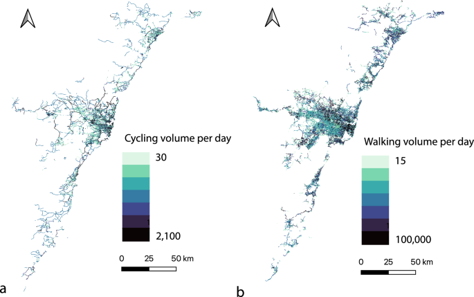
Link-level (a) cycling and (b) walking volumes.

Full size image

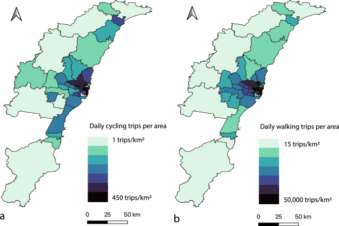
Number of (a) cycling trips and (b) walking trips per sq.km area.

Full size image

The presented walking and cycling modeling estimates suggest a total of 1.9 billion active transport trips per year occur across the study area. The NSW Household Travel Survey (HTS) data suggests that across the Sydney Greater Metropolitan Area (GMA) which includes Sydney Greater Capital City Statistical Area (GCCSA), parts of Illawarra and Hunter regions (including a total of 44 LGAs), 7.74 million walking trips occur per day without distinguishing between weekdays and weekends. The developed walking model (stacking regression) estimates that a total of 7.09 million walking trips occur per weekday and 6.67 million walking trips occur per weekend in the study area. The percentage difference between the model inference outcomes and HTS data is between 8.4% and 13.8%.

The NSW HTS data does not provide the number of cycling trips as a separate individual mode. Instead, it suggests 440,000 “other” trips per day that includes cycling, ridesharing, carsharing, etc. Optimistically assuming 50% of all the “other” trips in the HTS data are associated with cycling, there would be 220,000 cycling trips per day occurring across the study area. This estimate is comparable with the number of cycling trips per day estimated by our cycling model (stacking regression). Our developed cycling model estimates that a total of 260,000 cycling trips occur per weekday and 406,000 cycling trips occur per weekend in the study area.

Given the absence of network-wide street-level ground truth data, we cannot conclude with certainty the precise accuracy of the model inference outcomes. However, the validated results against NSW HTS data underscore the applicability and potential for the developed models to provide reliable insights and estimates for active transport trips, which can be instrumental in urban planning and policy-making aimed at enhancing pedestrian and cycling infrastructure.

Quality and quantity of input data are two critical elements in any machine learning modeling. Building upon the numerical results presented in the earlier sections, here we provide a thorough discussion on some of the major challenges and limitations of the presented modeling framework when scaled to large networks and using mobile phone-based and crowdsourced data.

The number of locations with observed walking and cycling count data are often limited. This affects the predictive power of the developed models and can introduce uncertainty in model estimations specially for areas with no observed count data. Also, the locations with observed walking and cycling count data are often not geographically diverse. Most official count locations are from high pedestrian and cycling activity areas (e.g. City of Sydney and City of Parramatta in our study) that naturally create a bias in the model outcomes. Therefore, future model development and improvement should try to maximize the geographical diversity and temporal coverage of the official count data locations as much as possible. Given both the walking and cycling models in this study were trained and tested on limited observed count data from relatively high walking and cycling activity areas, both models tend to overestimate the number of walking and cycling trips in low activity areas.

Generally, when a model is used for inference to predict walking and cycling counts across a large-scale network, representativeness of the training data becomes a significant challenge. In the presented cycling models in this study, the training dataset included links that are flatter, more densely populated, and with lower land use diversity compared to the entire network. This is evident from the distributions of the selected features in the cycling training dataset versus the entire network as shown in Fig. 6. Similarly in the estimated walking models, the training dataset also included links with smaller gradient, greater median income, more densely populated, and with greater land use diversity compared to the entire network. See Fig. 7. Despite the differences, the training data reasonably represents the NSW Six Cities Region for both walking and cycling models. Improving the representativeness of the training data is expected to improve the models inference quality.

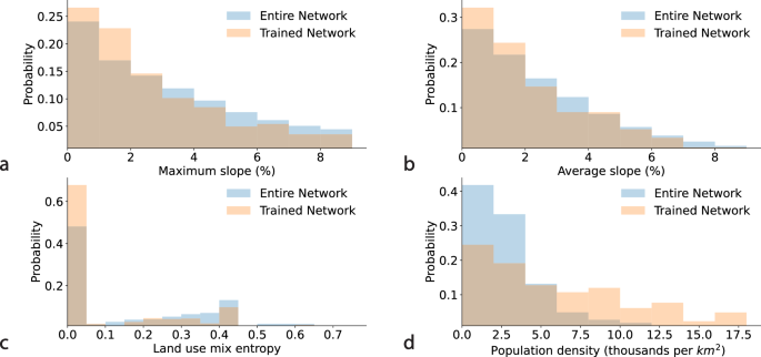
a Maximum slope, b average slope, c land use mix entropy, and d population density.

Full size image

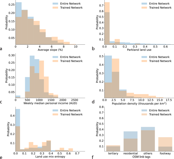
a Maximum slope, b parkland land use, c weekly median personal income, d population density, e land use mix entropy, and f OSM link tags.

Full size image

The representativeness of mobile phone and crowdsourced data plays a pivotal role in the accuracy and reliability of machine learning models. However, the inherent characteristics of these data streams, such as their spatial and temporal sampling bias, could be subject to change over time due to various factors including shifts in technology usage patterns, demographic changes, and infrastructure developments. Given the dynamic nature of these data sources, the representativeness of the data may evolve, potentially impacting the performance of existing models. For instance, changes in mobile phone usage patterns or the emergence of new crowd-contributed platforms could alter the spatial and temporal distribution of data points, leading to shifts in the underlying patterns of walking and cycling. To mitigate the risk of model degradation and ensure the continued relevance of the estimations for active transportation planning and operations, it is imperative to establish a framework for periodic model re-training and re-testing. This involves updating the training dataset with new observed walking and cycling count data collected across as many locations as possible within the study area. By periodically retraining the models, practitioners can adapt to changes in data representativeness and maintain the models’ accuracy and robustness over time. Additionally, re-testing the models against new data allows for the assessment of their performance under evolving conditions and facilitates the identification of any necessary adjustments or recalibrations.

Strava cycling data does not include links with number of cycling trips smaller than 5 per day. This potentially creates many links with no data in any single day that may have low cycling activity. See Fig. 8. A potential solution to mitigate the impact of links with no data is to look at a longer period (for example one year’s worth of Strava raw data) and take an average Strava cycling count for each link. Same limitation applies to the mobile phone-based walking count data in which links with very low walking volume are not included and reported because of larger uncertainty in the estimates. This uncertainty essentially carries over to any model estimation based on mobile phone and crowdsourced data.

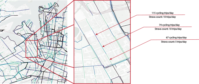
An example illustration of the missing links in the network and inconsistencies in link-level estimations in a selected corridor.

Full size image

Link-level estimation of walking and cycling volumes could also create potential inconsistencies in some streets or corridors that are made of multiple smaller links where the smaller links have different attributes such as slope or associated population or land use characteristics. See Fig. 8. While mobile phone and crowdsourced data (e.g. Strava and mobile phone-based) may offer insights on some major walking and cycling corridors, when the link-level model estimates are applied, a uniform normalization should not be expected across the space (e.g. route or corridor). For example, a corridor could be a major route for recreational cycling trips given Strava user types but when the developed model corrects the Strava raw data to the whole population, some parts of the corridor depending on its land use and population characteristics may not remain a major route for the whole population. Thus, the model outcomes may no longer presents similar distinct corridors and routes as in the Strava or the mobile phone data.

A major limitation of the developed walking and cycling models is that they are purely data-driven and for operations applications rather than long-term planning. The developed models do not include any behavioral theory capturing travelers’ behavior, route and destination choices, or user preferences. An interesting direction for future research is development of a strategic active transportation network planning model empowered by a range of behavioral demand and supply models as well as machine learning models.

Observed walking and cycling count data

Official observed walking and cycling count data are obtained from a range of sources including Transport for NSW open data hub, City of Sydney open data hub, and City of Parramatta Pedestrian and Cyclist Dashboard among others. A total of 27,631 walking count records and 18,535 cycling count records between 2013 and 2023 across 766 sites are collated. See Fig. 9. In this study, we assume the observed count data represent the ground-truth. If there is an error in the ground-truth data, additional approaches should be designed and put in place to account for the error in the modeling. The spatial diversity of the observed count locations is of outmost importance in the presented modeling approach and can have significant impacts on the quality of the modeling outcomes, which will be discussed in detail later in the manuscript.

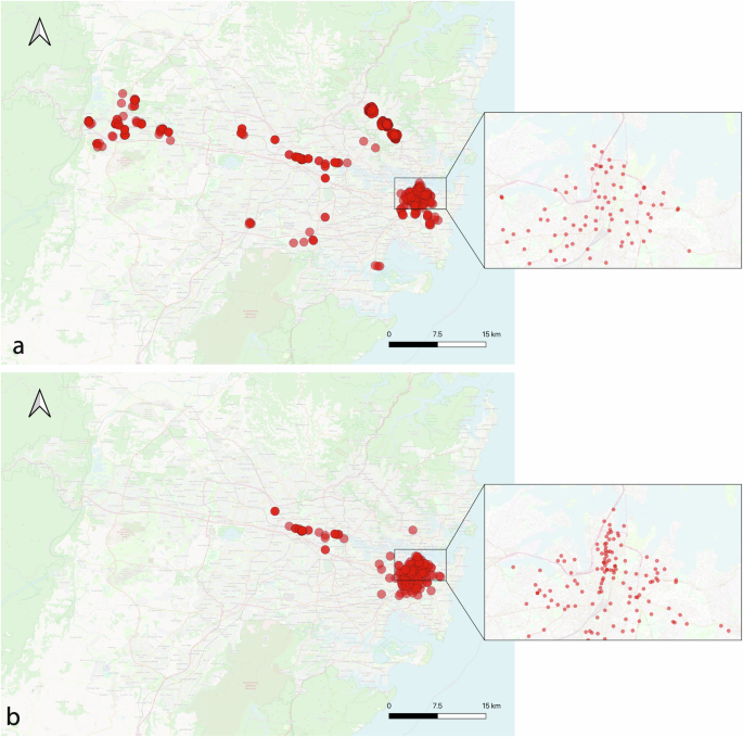
a 634 walking and b 160 cycling count locations across the study area.

Full size image

Mobile phone and crowdsourced data

We use link-level estimates of walking counts from a private telecommunications company that takes billions of data points generated daily by mobile phone devices across Australia, cleans, aggregates, and anonymizes it using their proprietary analytics framework to generate mobility insights including aggregated and link-level estimates of walking trips. We also use link-level cycling counts from Strava Metro. Strava Metro derives data from Strava fitness app’s GPS records and offers both aggregated and link-level cycling counts. Both data types have been widely used and explored in the literature^17,21,26,27 with well-documented issues in relation to sampling bias, localization error, etc.

Population and land use data

We use population and land use data from Australian Bureau of Statistics (ABS) Census 2021 at the Statistical Areas Level 1 (SA1s) level across the study area. SA1s are geographic areas in Australia created from whole Mesh Blocks, totaling 61,845 zones without gaps or overlaps. They are designed to maximize geographic detail for Census data, with each SA1 having a population of 200 to 800 people, representing urban or rural characteristics. Here, we specifically work with the following population and land use data that are shown to have significant association with the bias in the crowdsourced and mobile phone data^12,14 in the context of walking and cycling:

1. 1.

   Population density (person/sq.km)

2. 2.

   Person weekly median income (AUD)

3. 3.

   Land use mix entropy

Land use mix entropy (LUM) is a measure of the heterogeneity/homogeneity of land uses which uses the areas of different land use categories within each SA1 polygon to calculate an index between 0 and 1. An index of 1 represents a completely mixed land use while an index of 0 represents a single use land within the SA1. LUM is calculated based on Christian et al.²⁸ work as follows.

where ({p}_{i}) is the proportion of the SA1 covered by the land use class (i) against the summed area for all land use classes and (n) in the number of land use classes. Here, we use all available land use classes in the ABS Census data including residential, industrial, education, parkland, and hospital/medical.

Household Travel Survey (HTS) data

The NSW HTS is a continuous data collection initiative started in 1997/98 that focuses on personal travel behavior within the Sydney Greater Metropolitan Area. It involves randomly selecting residents from occupied private dwellings in the survey area, with approximately 2,000-3,000 households participating annually. The survey collects data on all trips including active transportation made over a 24-hour period by members of participating households, producing annual estimates weighted to the ABS’ estimated resident population for an average weekday.

Air quality, climate, and topography data

Air quality data including PM2.5, PM10 and visibility (NEPH) information are obtained from NSW Government Department of Planning, Industry and Environment. Climate data including precipitation and temperature are obtained from the Australian Bureau of Meteorology. Each link in the study networks is then linked with the closest weather station and air quality station to obtain precipitation (mm), temperature (C), PM2.5 (µg/m3) and other air quality metrics. Topography information is obtained from Geoscience Australia, Digital Elevation Map with which we estimate an average and maximum slope for each link in the study networks.

See Supplementary Table S1 (Supplementary Material) for a summary of all variables, their associated spatial and temporal aggregation, and data sources used in this study. All temporal resolutions are converted to the daily level. Observed walking and cycling counts, sourced from various origins and initially aggregated either hourly or daily, are converted to daily measurements for model training and testing. Mobile phone-based walking counts and Strava cycling counts are also recorded on a daily basis. Precipitation is measured as accumulated rainfall over the previous 24 h in millimeters, aligning with daily data collection. Minimum and maximum temperatures are recorded daily. PM2.5, PM10, and NEPH values represent 24-h averages, derived from hourly measurements and thus are considered at the daily level. Other features, including population density, median personal income, maximum slope, average slope, land use mix entropy, percentage of ‘walk-linked’ trips, points of interest (POI) density, and OpenStreetMap (OSM) tags, exhibit negligible temporal variations. Notably, data for population density, median personal income, and land use mix entropy are derived from Census data, calculated every five years. The percentage of ‘walk-linked’ trips is sourced from NSW Household Travel Survey data, updated annually. POI density and OSM tags are sourced from the OSM community, which lacks an official release schedule.

All variables are also converted from various spatial aggregation levels to the link level. Observed and mobile phone-based walking and cycling counts are originally recorded at the link level. The average and maximum slopes, calculated using high-resolution DEMs at either 5 m or 30 m, are determined at the link level. Precipitation, minimum temperature, and maximum temperature data are divided into catchment areas based on the closest station to each link, as illustrated in Fig. 10. Similarly, PM2.5, PM10, and NEPH measurements are distributed across several catchment areas, aligned with the nearest station to each link. Population density, weekly median personal income, land use mix entropy, and POI density are aggregated at the SA1 level, while the percentage of ‘walk-linked’ trips is aggregated at the LGA level. These variables are then assigned to each link in the network based on the SA1 or LGA level to which the link belongs.

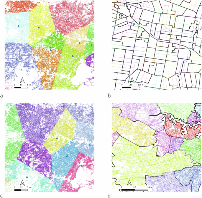
a Catchment area of air quality stations as blue triangles and b SA1 boundaries in black lines overlaid on cycling links in the study network; c Catchment area of weather stations as blue triangles and d LGA boundaries in black lines overlaid on walking links in the study network.

Full size image

Descriptive statistics of the input data

Tables 6 and 7 provide further details on the quantity, temporal coverage and descriptive statistics of the input data used in development of the walking and cycling models, respectively. In Table 5, focusing on the walking model, various datasets are outlined, including official observed walking counts, mobile phone-based walking counts as well as some of the climate and air quality metrics. The number of records, temporal coverage (from and to dates), and data sources are specified for each category, providing essential details for better understanding the input data. Table 6, dedicated to the cycling model, follows a similar structure, featuring observed cycling counts, Strava cycling counts, as well as data on precipitation, temperature, and a few of the air quality metrics, with corresponding records, temporal coverage, and additional notes on number of associated weather and air quality stations that the data were collated from.

Tables 7 and 8 provide further descriptive statistics (minimum, mean, median, maximum, and standard deviation) of the input data for the walking and cycling models, respectively. The largest observed walking and cycling count across the study area was 194,400 pedestrians per day and 1358 cyclists per day, respectively. The mean observed walking and cycling count was 4823 pedestrians per day and 188 cyclists per day. The statistics suggest that the majority of the observed count data are located in relatively high pedestrian and cycling activity areas that may impact the quality of the model training and testing that will be further discussed later in the manuscript.

Feature selection and importance analysis

To identify which features should be further explored and included in the model training, we use domain-specific knowledge, insights offered from the published literature^10,11,12 and a commonly used technique known as Least Absolute Shrinkage and Selection Operation (LASSO). Tables 9 and 10 provide a summary of the LASSO analysis as well as estimated variance inflation factor (VIF) to assess variables multicollinearity across all the variables initially considered in the modeling. Generally, higher LASSO coefficient suggests a greater feature importance. VIF equal to one means variables are not correlated and multicollinearity does not exist in the model.

The LASSO analysis for the walking model reveals that the mobile phone-based walking count, population density, and Place of Interest (POI) density are the most influential features, while other variables such as the weather and climate indicators have lower importance. The VIF indicates low multicollinearity. For the cycling model, Strava cycling count, population density, and slope are crucial, with weekday/weekend classification and bicycle infrastructure also significant. COVID-related factors show moderate importance. VIF values suggest minimal multicollinearity. Overall, the findings guide feature selection, emphasizing key variables for model training and testing in the next section.

Final models’ variable selection

Following an extensive model training, validation and testing the following variables are kept in the final walking and cycling models. See Tables 11 and 12. The LASSO analysis confirms that the selected variables for the final models are of significant importance with high LASSO coefficient and no strong multicollinearity except a few variables in the walking model. As expected, the mobile phone-based walking count and Strava cycling count are the most important input feature in the walking and cycling models, respectively based on both LASSO and GINI coefficients. Generally, if VIF > 10, then multicollinearity is high. Note that multicollinearity does not reduce the predictive power or reliability of a model as a whole; it only affects estimations regarding individual predictors. In other words, a multivariable regression model featuring collinear predictors can provide insights into the overall predictive performance of the entire set of predictors concerning the outcome variable. However, it might not yield reliable findings regarding any specific predictor or identify which predictors overlap with others in terms of redundancy.

The only selected variables in the walking model that show signs of high multicollinearity include the percentage of “walk linked” trips and median personal income, as well as minimum temperature and maximum temperature. The percentage of “walk linked” trips and median personal income are likely to have correlation with population density and land use mix entropy in Sydney. Maximum and minimum temperatures are also highly correlated in a single day. Despite the existence of multicollinearity, we have kept the variables in the model as they do not affect the predictive power of the developed models.

Spatial and temporal cross-validation

Cross-validation (CV) splits data into different sets to avoid model overfitting and bias toward known locations. CV generally serves dual purposes: model selection and model assessment, each requiring distinct approaches. Despite the differences between these processes, there has been a tendency to equate the cross-validation error obtained for the optimal model during selection with the evaluated model performance. Common methodologies in the literature include double CV and nested CV. Double CV involves an outer loop for model selection, with parameter tuning occurring within an inner loop^29,30. Nested CV consists of an outer loop for model selection and an inner loop for hyperparameter tuning or feature selection^31,32,33. In this study, we propose a simplified double CV and demonstrate its applicability and performance within the walking and cycling volume estimation context.

The proposed simplified double K-fold CV is structured into two primary steps: parameter tuning conducted within the inner loop and model selection within the outer loop, as shown in Fig. 11. For the walking model, the dataset undergoes spatial splitting, allocating 20% to form the test dataset and 80% to constitute the calibration set, termed the outer loop. Within this outer loop, further calibration subsets are created, each with around 20% of the data omitted, forming what is referred to as the training dataset. Subsequently, each training dataset is further partitioned both spatially and temporally into 10 distinct calibration sets, constituting the inner loop of the proposed cross-validation method. Consequently, within each 80% portion of the dataset, there are nested 10 sub-folds, iterated 10 times. Similarly, for the cycling model, we split the original dataset into 10% to form the test dataset and 90% to constitute the training set as the outer loop. Then, 90% of the dataset is further divided into 10 sub-folds for cross-validation and parameter tuning. For the voting regressor, hyperparameter tuning is performed on the inner training dataset after the spatial split.

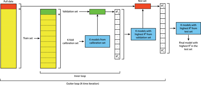
The proposed approach consists of an inner and an outer loop. In the inner loop, K-fold calibration and validation is performed. In the outer loop, testing is performed K-times.

Full size image

The inclusion of extensive CV in model development, particularly in the presence of substantial spatial and temporal heterogeneity within observed data, is crucial for strengthening the model’s robustness and applicability, especially in large-scale networks. This methodological approach enables a more robust exploration of the inherent variations in diverse walking and cycling count data sampling locations and times. This rigorous evaluation safeguards the developed models against overfitting, enhances pattern discernment across locales and time frames, and serves as a vital quality control measure.

Identifying model estimation outliers

Given both walking and cycling models are trained mostly with data from relatively high pedestrian and cycling activity locations, the models tend to suffer from over-estimation in low pedestrian and cycling activity areas. To identify links with over-estimated walking and cycling counts, we adopt the “Kneedle” algorithm³⁴ to identify the outliers. The Kneedle algorithm is applied to the distribution of the ratio of the model estimates over the mobile phone-based walking counts or Strava cycling counts and systematically estimates the “elbow” point, estimated as 8 for the walking model and 16 for the cycling model. The estimated elbow point can be used as a cutoff line for outlier identification represented by the heavy tail of the distributions show in Fig. 12.

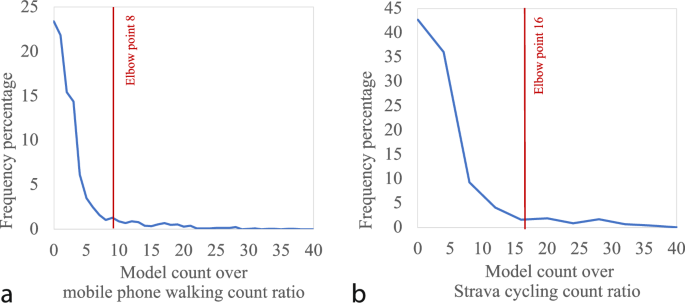
Distribution of the (a) ratio of the estimated link-level walking counts over the mobile phone-based walking counts and (b) ratio of the estimated link-level cycling counts over Strava cycling counts.

Full size image

The estimated elbow points are used to identify links in the network with excessive over-estimation. With the estimated elbow point of 8 for the walking model, about 10% of the link estimates across the entire study area are identified as outliers. While with the estimated elbow point of 16 for the cycling model, only less than 6% of the link estimates across the network are identified as outliers. The analysis suggests that while the developed walking model suffers from over-estimation, the cycling model estimates are more reasonable. The overestimation evident in the walking model signifies a tendency towards amplifying pedestrian counts, particularly in locales characterized by minimal pedestrian activity. This tendency introduces a susceptibility to inaccuracies in predictive outcomes. The cycling model, however, exhibits more robust estimations, indicative of enhanced reliability in forecasting cycling counts across a spectrum of locations. This difference emphasizes the need to be cautious when using the walking model in areas with low pedestrian activity, while the cycling model proves to be a more reliable option for various situations.

A few practical solutions to tackle the issue of the over-estimation in the walking model include applying a hard upper bound constraint on the ratio of the model walking count estimates over the mobile phone-based walking counts. An alternative approach is to replace the estimation of the walking counts from the proposed stacking regression model with the base model presented earlier in the paper. This would mitigate the impact of the over-estimation issue for the identified subset of links across the network without affecting the model estimations in areas where over-estimation is not present or not as significant that is about 82% of the links in the network.

Machine learning models

The study estimated and examined a range different machine learning models including:

• Linear regression

• Support vector regression (SVR)

• Gaussian Naïve Bayes

• Tree regression

• Multi-layer perceptron (MLP)

• Adaptive Boosting (AdaBoost)

• Gradient Boosting regression

• Random Forest

• Voting regressor (incl. linear regression, MLP and Random Forest)

• Stacking regressor (incl. linear regression, Random Forest, Gradient Boosting, AdaBoost)

SVR is a machine learning algorithm that uses support vector machines to perform regression tasks. It aims to find a hyperplane that best fits the data while minimizing the error. Gaussian Naïve Bayes assumes that features are conditionally independent given the class label and follows a Gaussian (normal) distribution. Tree regression involves constructing a decision tree to model the relationship between features and the target variable in a regression task. MLP is a type of artificial neural network with multiple layers of nodes (neurons) organized into input, hidden, and output layers. It is widely used for classification and regression. Ensemble learning involves combining machine learning algorithms to address regression challenges. Ensemble learning strategically blends various ML models to enhance performance compared to a single model. AdaBoost is an ensemble learning method that combines the predictions of weak learners (often simple decision trees) to create a strong learner. It assigns weights to data points and focuses on misclassified samples to improve performance iteratively. Gradient Boosting Regression is also an ensemble learning technique that builds a series of weak learners (usually decision trees) sequentially. It aims to correct errors made by previous models by assigning more weight to misclassified observations. Finally, voting and stacking regressors are also types of ensemble learning models. Stacking aims to learn the optimal way to combine the predictions of the base models while Voting focuses on aggregating the predictions to make a final prediction.

Converting link level estimates to aggregate measures

To estimate the total number of walking and cycling trips in the study area, we aggregate and convert the link-level count estimates across all links as follows.

where ({d}_{w}) and ({d}_{b}) denote average walking and cycling trip distance, respectively. ({gamma }_{w}) and ({gamma }_{b}) denote effective walking and cycling distance factors, respectively. ({{ADPV}}_{i}) represents the estimated Average Daily Pedestrian Volume for link (i) while ({{ADBV}}_{i}) represents the estimated Average Daily Bicycling Volume for link (i). ({l}_{i}) represents the length of link (i). Note that (sum _{i}{{ADPV}}_{i}.{l}_{i}) represents the total walking kilometers traveled and (sum _{i}{{ADBV}}_{i}.{l}_{i}) represents the total bicycle kilometers traveled across the study area. Here, we assume that the average walking trip distance is 1 km based on the NSW HTS data and the average cycling trip distance is 4.7 km based on the Sydney Cycling Survey 2011 data. We also define the effective distance factor as the average percentage of a link length traversed by a pedestrian or cyclist. Given the short distance nature of most walking and cycling trips, the entire length of a link may not be entirely traversed by a pedestrian when walking from an origin or to a destination, especially when the walking and cycling trips are inferred through the motion of mobile phones. Here, we assume an effective distance factor of ({gamma }_{w}=0.5) for the walking model and an effective distance factor of ({gamma }_{b}=1) for the cycling model. Assuming a larger effective distance factor will increase the estimated total aggregated number of trips.