Operating principles of interconnected feedback loops driving cell fate transitions

Introduction
Understanding the principles underlying the emergence of diverse and functionally distinct cell types within a living organism is fundamental to unraveling development and disease progression mechanisms1,2,3. As cells undergo proliferation and organize into tissues, their molecular characteristics undergo discrete, step-like changes, leading to the generation of various sequences of unique cell states. These transitions ultimately result in the differentiation of specific functional cell types4. Consequently, the development of cells can be conceptualized as the formation of branching cell lineages that yield greater diversity and increasingly specialized cell types5. This developmental trajectory, though driven by gene interaction networks, is also significantly influenced by intercellular signaling among differentiating cells, rendering the process nonautonomous yet self-organizing6. At each branch point in a cell lineage, cells face choices between alternative, distinct cell types, with each decision referred to as a cell fate determination. The high throughput single-cell transcriptional profiling techniques and mathematical/computational models of transcription networks have profoundly unveiled some of the complexity in cell fate decisions7,8,9. These models bolster the notion that cell fates can be conceptualized as the stable states of a multistable gene regulatory network (GRN)10. Recent advances have highlighted that the topology (structure) of GRNs can substantially dictate the fate decisions of cells and, have, therefore identified specific markers for multistability (multiple alternative states)11,12,13. For instance, from the network topology perspective, studies have shown that the presence of autoregulated genes14, positive feedback loops15,16,17, and their interconnections18 are hallmarks of multistability. Further, from the mathematical modeling perspective, some recent studies have reported that multistable systems have a sufficient time delay between gene interactions19,20, and regulatory functions modeling gene interactions are always convex21.
One of the simplest networks underlying binary fate decisions is the toggle switch consisting of two mutually repressive genes, say X and Y, forming a double-negative (positive) feedback loop. Under ideal conditions, the toggle switch dynamics converge to one of the two steady states, (({X}^{{ON}}), ({Y}^{{OFF}})) or (({X}^{{OFF}}), ({Y}^{{ON}})), thereby explaining the “either/or” choice between the two cell fates20. Practical examples of such circuits are found in both development and diseases. For instance, during hematopoiesis, ({GATA}1) and ({PU}.1) mutually repress and drive a common myeloid progenitor to either erythroid lineage (({{GATA}1}^{{ON}}), ({{PU}.1}^{{OFF}})) or a myeloid lineage (({{GATA}1}^{{OFF}}), ({{PU}.1}^{{ON}}))22,23,24. Similarly, mutual repression between ({Ptf}1a) and ({Nkx}6) controls the branch point in the fate map where a pancreatic progenitor decides between two lineages: exocrine (({{Ptf}1a}^{{ON}}), ({{Nkx}6}^{{OFF}})) and endocrine ({({Ptf}1a}^{{OFF}}), ({{Nkx}6}^{{ON}}))5,25(.) On the other hand, a prominent example of cell state transition in diseases is the epithelial-mesenchymal transition (EMT)-induced metastasis of carcinoma, which is primarily driven by double-negative feedback loops formed between miR200 (micro-RNA) – epithelial marker gene, and Zeb (mRNA) – mesenchymal marker gene, family members26,27. The EMT confers non-motile epithelial tumor cells with the characteristics of mesenchymal cells, which are more migratory and invasive. The migrating cancer cells undergo a reverse mesenchymal-to-epithelial transition (MET) to seed metastatic tumors27,28. This circuit explains the “go or grow” mechanism of cancer cells in which the “go” phenotype (viz. migratory and invasive) is enabled by (({{miR}200}^{{OFF}}), ({{Zeb}}^{{ON}})) and the “grow” phenotype (viz. proliferative) is enabled by (({{miR}200}^{{ON}}), ({{Zeb}}^{{OFF}}))29,30.
While positive feedback loops (PFLs) are the cornerstone for binary cell lineage decisions, in practice, the robust cellular function and reliable cell decision require diverse cross-talk among the genes, which is manifested through interconnected feedback loops31,32. For instance, compared to a single PFL, two interconnected PFLs significantly increase the range of cellular conditions in which bistability is observed5,32. These interconnected positive feedback loops are widespread in biological systems, including stepwise lineage decision of CD4 + T cells, cell cycle regulation, neuronal cell fate decision, calcium signal transduction, B cell fate specification, and EMT17,31,33,34,35,36,37,38. A thorough understanding of the design principles of the interconnected PFLs is therefore crucial to understanding robust cell functioning, cell fate decisions, and diseases such as EMT-induced metastasis of carcinomas.
Here, we identify numerous topologically distinct interconnected PFLs intertwined in complex biological networks implicated in EMT-enabled carcinoma phenotypic transition and CD4 + T cell differentiation11,30,37,39,40,41,42. We define these interconnected PFLs as high-dimensional feedback loops (HDFLs), a term coined by combining definitions from Ahrends et al. 35 and Nordick and Hong (2021)33,35. We find that these HDFLs have three types of “global” structures (topology): (i) serial topology, in which toggle-switches (positive feedback loops formed by two mutually antagonistic genes) are connected serially like a chain; (ii) hub topology, in which several toggle switches are incident on one common toggle switch to form a hub network; and (iii) cyclic topology, in which toggle switches are connected end-to-end forming a loop (Fig. 1). We investigated multistability as an emergent property of these networks by analyzing their steady-states space (see methods). Our findings show that serial and hub HDFLs have contrasting dynamics, highlighting a new direction to further our understanding of the mechanism leading to multiple alternative states. The serial HDFLs tend to exhibit multiple alternative states, which become more pronounced as the network size grows larger. A decline in the frequency of monostable steady states compensates for the increase in higher-order stability. In contrast, in hub HDFLs, the steady states space is restricted to mono- and bistability, and as network size becomes larger, we observe a sharp incline in the frequency of bistable steady states, which is compensated by a sharp decline in mono-and Higher-order stability. Moreover, irrespective of network topology, autoregulations (self-activated genes) shift the steady state distribution (SSD) towards Higher-order stability, which becomes more prominent in serial networks compared to hub networks. This implies that autoregulations result in partial loss of the influence of topology on network dynamics.

In serial networks, multiple toggle switches are connected end-to-end. In hub networks, multiple nodes interact with a common node. In cyclic networks, a closed loop is formed between the network nodes. Each network is assigned a unique color code for comparative analysis and a name reflecting the type of topology and the number of nodes in the network. For instance, S3 is a Serial network with three nodes, and H4 is a Hub network with four nodes, and so on. SH5 has a hybrid Serial-Hub (SH) topology with five nodes. The toggle triad (TT), toggle square (TS), and toggle polygon (TP) networks have cyclic topologies with three, four, and five nodes, respectively. Networks with annotated nodes are real biological networks and those without annotations are “synthetic” networks. Lines with a bar denote inhibition/repression. Mutual inhibition between two nodes forms a toggle switch.
Next, we constructed all possible topologically distinct HDFLs with three, four, and five nodes that allowed us to introduce “synthetic” networks such as “toggle square” and “toggle pentagon” (Fig. 1). We asked whether HDFLs with the same number of nodes or toggle switches engaged in different topologies can have comparable steady-state space. Our analysis reveals that HDFLs with an equal node count or toggle switch count operate differently, highlighting the crucial role of network structure in governing the dynamics. However, we found that cyclic and serial networks with the same node count have comparable dynamics and that cyclic topology further amplifies the frequency of Higher-order stability observed in serial networks. To identify targets in the network topology that can restrict the state space to lower order, we found that edge sign reversals (converting repressions into activations) that increase negative feedback loops are more effective than edge deletions that reduce PFLs. Finally, we unraveled the distinct effects of these network perturbations in HDFLs with- and without self-activations. While in networks with no self-activated genes, a particular type of perturbation at any position has the same impact, in networks with self-activated genes, a perturbation involving the self-activated node substantially increases (reduces) the likelihood of monostable (bistable) states. Together, these results highlight the interesting association of network structure with the phenotypic outcome and how autoregulations partially “set free” the dynamics of networks from the topological control. As these networks drive cell fate transitions in development and disease such as metastasis and since multistability can be mapped to phenotypic heterogeneity, our results link the structure of HDFLs with the phenotypic heterogeneity while also suggesting measures to maneuver the structure to control phenotypic plasticity.
Results
A “tug of war” between serial and hub networks as they pull on the opposite ends of the stability axis
Interconnected toggle switches are crucial components of complex cell lineage decision networks, particularly cell fate transition networks governing EMT and MET. Therefore, understanding the operational principles of these recurrent network structures can offer promising ways to decode cellular differentiation processes, cell fate switching, and heterogeneity of carcinomas. We curated numerous such networks from the literature, and based on their “global” structure, we categorized these into three types: serial (S3, S4, and S5), hub (H4 and H5), and cyclic networks (TT, TS, and TP). In serial networks, multiple toggle switches are connected serially or end-to-end to form an extended chain of toggle switches. In contrast, in hub networks, multiple toggle switches are incident on a common central node to form hub-type networks. With an exception, SH5 has a hybrid serial/hub topology since an additional toggle switch is incident on the ZEB1 node besides the linear chain of three toggle switches (Fig. 1). To understand whether these three network families fundamentally differ in functioning, we investigated the emergent dynamics of these unperturbed or “wild-type” (WT) networks and their self-activated (SA) counterparts using an ordinary differential equation (ODE) based modeling approach implemented in a robust computational algorithm, RAndom CIrcuit Perturbation (RACIPE)39,43 (see Methods).
As depicted in Fig. 2A, we observe distinct SSD trends in the serial and hub networks as network size becomes large. The three-node network, S3, exhibits mono- and bistability and has a negligible chance (<2%) for tristability (Fig. 2A). This shows that, in terms of the order of stability, two interconnected toggle switches behave much like a toggle switch network, which in ideal conditions also exhibits at most two stable states (Fig. 2A). However, a deeper look at the frequencies of the states reveals the role of the additional toggle switch in the S3 network. While the toggle switch network exhibits 60% more monostable states than bistable states, in the S3 network this difference reduces to 15% (Fig. 2A). This observation suggests that an additional toggle switch in the S3 network substantially increases the range of cellular conditions in which bistability can be observed. This finding is in line with experimental data showing that two positive feedback loops result in a bistable behavior over a broad range of inducer concentrations32. In the S4 network, which consists of three toggle switches, we observe a further reduction in monostability and an increase in bistability (Fig. 2A). This network also exhibits a substantial percentage of tristability (three steady states). We asked whether increasing network size by adding more toggle switches serially can further reduce the frequency of monostable states and increase the frequency of tristable and other higher-order states. To answer this, we found that in a relatively larger serial network, S5, monostable states decline sharply which is compensated by a sharp increase in tristable states, together with some tetrastable (four) states (Fig. 2A). On the other hand, as we switch to hub networks, the SSD of H4 settles around mono-and bistability and bistability is more likely to occur than monostability (Fig. 2A). As the network size increases, we observe in the H5 network a further drop (~10%) in monostable states compensated by an increase in bistable states while the tri-and higher-order states almost disappear. This begs the question: do serial and hub networks pull on the lower and higher order ends of the stability axis, respectively? To answer this, we tested our hypothesis on larger (generic) serial and hub networks each having 10 nodes (Supplementary Fig. 1). Strikingly, our findings show that a 10-node serial network has almost equal probability (~20%) to exhibit bi, tri, and tetrastable states, which is nearly double the probability of monostable states (~10%) (Supplementary Fig. 1A). On the other hand, a 10-node hub network has almost an 85% chance for bistability and a 15% chance for monostability (Supplementary Fig. 1B). Our results are thus consistent in larger networks, and we conclude that ST topology favors higher-order stability that increases (and saturates) with the number of nodes in the networks. In contrast, hub topology favors lower-order stability and bistability becomes dominant in larger hub networks. These findings thus identify design principles of HDFLs exhibiting two and multiple alternate states.
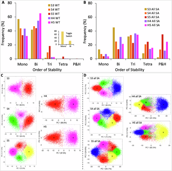
The SSD of wild-type serial and hub networks (A) and their self-activated (SA) counterparts (B). Gene expression data projected on the 1st and 2nd principal component axis for WT networks (C) and their self-activated counterparts (D). Each dot (of 10,000 dots) in the plot is a stable steady state (or phenotype) of a model corresponding to a specific parameter set. K-means clustering was used to group locally identical states and identify distinct “global” states that represent distinct cell states (phenotypes) a network can support (see methods for details). The number of phenotypes increase as network size increases serially (say, from S3 to S5) and remains unchanged as network size increases and becomes hub (say, from S3 to H4 to H5). Mono, Bi, Tri, and Tetra denote monostable, bistable, tristable, and tetrastable states. Penta-and higher (P&H) collectively denotes five and up to ten states, respectively. “WT” implies a wild-type (without any perturbation) network. “All SA” means all nodes are self-activated. “X” in scatter plots denotes the centroids of the clusters. Cluster colors have no correspondence with the colors used to designate networks.
To connect these findings to the state space dimension, we projected the in silico gene expression data of these networks on the first two principal components (Fig. 2C). We employed k-means clustering to identify the feasible states (clusters) allowed by each of these networks (see methods). Each dot in the plot represents a phenotype (or a steady state corresponding to each parameter set in the model) and phenotypes with similar gene expressions are grouped to form clusters. The total number of clusters determines the number of viable phenotypes exhibited by a network. We observe that under variable cellular conditions (variable biochemical parameters) S3, S4, and S5 networks can exhibit two, three, and four distinct phenotypes, respectively, while hub networks, regardless of their size, can exhibit at most two distinct phenotypes (Fig. 2C, Supplementary Fig. 1). We thus show that multiple alternative states exhibited by complex transcriptional networks can be facilitated by serial topology. These findings, therefore, reveal opposing roles of the serial and hub topology of networks in exhibiting alternative fates during cell state transition and highlight that hub topology (one manifestation of which can be higher complexity) can work against and prevent the occurrence of numerous states. Our findings elucidate how the structural composition of HDFLs can influence the dimensionality of state space and concomitant cell fate ‘canalization’ during lineage decision. Interestingly, our observations corroborate with previous studies showing that large networks (which resemble our hub HDFLs), despite their complexity, exhibit only a limited number of viable steady states, a phenomenon termed ‘canalization’ of complex networks44,45,46,47.
Also, we investigated the impact of self-activations (which are very common in gene regulation) on the dimension of state space. To analyze this, we assumed that each gene (node) can activate its transcription, and therefore, we constructed the self-activated counterparts of these networks. The SSD of networks with all self-activated genes revealed interesting roles of autoregulations in serial and hub networks. As depicted in Fig. 2B, for each network, the SSD peak is shifted towards higher-order stability as compared to their WT counterparts (Fig. 2A). A deeper analysis reveals that with the addition of each self-activation, the SSD peak gradually shifts to higher-order stability and a linear relationship between the number of SA genes and the order of stability in each network is evident (Supplementary Fig. 2). Interestingly, irrespective of the topology, this trend persists across the networks. This finding is further supported by the gene expression data, which shows that all self-activated HDFLs exhibit more alternative states (represented by distinct clusters) than their WT counterparts (Fig. 2D). We thus report that autoregulations “liberate” network dynamics from the topological control and evoke a uniform response across the networks by shifting the dynamics to higher order stability.
Topologically distinct HDFLs with an equal number of nodes operate differently
Of all the “biological” HDFLs reported in Fig. 1, we notice that several topologically distinct networks have an equal number of nodes. For instance, S3 and TT each have three nodes, S4 and H4 have four nodes, and SH5 and H5 are five-node networks, integrated through different topologies although. We asked two interesting questions: (i) How many topologically distinct HDFLs can be constructed with three, four, and five nodes, and (ii) Would the SSD of HDFLs with the same number of nodes be similar? We started with three nodes and found that only two distinct HDFLs can be formed: one is the linear chain of three nodes connected with two toggle switches (S3) and the other is a network whose three nodes are the vertices of a triangle connected by three toggle switches, called toggle triad (TT). Likewise, we can only construct three structurally distinct four-node HDFLs, viz. S4, H4, and toggle square (TS), and only four structurally distinct five-node HDFLs, viz. S5, H5, SH5, and toggle polygon (TP) (Fig. 1). This is how “synthetic” networks (in the sense that we don’t have biological examples of these networks) come into play in this study. These cyclic networks (i.e., TT, TS, and TP) have recently been studied in detail by Duddu et al.48 and Kishore et al.49.
We did a comparative steady-state analysis of networks in each group. When considering three-node networks, we observe that mono-and bistable frequencies in S3 and TT differ slightly and the SSD peak for both networks is skewed towards mono-and bistability. We also notice some tristable states (<10%) emerging in TT, which can be attributed to an extra toggle switch in TT (Fig. 3 A1). Among the four-node networks, S4 and H4 have comparable mono-and-bistable frequencies but significant differences (~3 times) in tristable frequencies (Fig. 3 B1). On the other hand, we find a sharp decline in monostable frequencies in the TS network compensated by an increase in bi-and-tristable frequencies. The tristable frequencies of S4 and TS networks are almost the same. This demonstrates that both serial network S4 and cyclic network TS push for higher-order stability and thus operate differently than the hub network H4. In the five-node networks, it is evident that S5, SH5, and TP have comparable mono, bi, and tristable frequencies, and as expected H5 network has the highest/lowest bistable/tristable frequencies due to its hub topology (Fig. 3C1). Also, the SSD of TP shows the emergence of higher tri-and tetrastable solutions compared to other networks in the group. This shows that like TS, the cyclic network TP also operates closer to the “pure” serial network, S5, than hub network H5 or serial-hub network SH5. This difference in dynamics is also reflected in scatter plots characterizing the distinct states allowed by a network for 10,000 different parameter sets (Supplementary Fig. 3). From the plots, it is evident that among three, four, and five-node networks, cyclic networks exhibit an extra alternative state than serial networks, and the hub networks exhibit just two states (Supplementary Fig. 3). We thus find that all the topologically distinct networks constructed from a given (same) number of nodes result in a different number of states, typically governed by the specific topology.
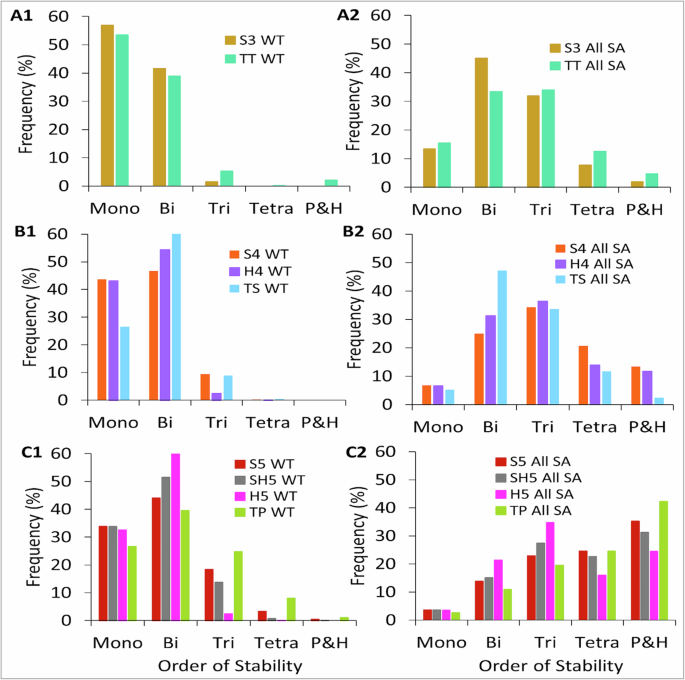
A1 Three-node networks showing almost overlapping SSD. B1 Four-node networks show non-overlapping SSD. Cyclic network TS functions like a serial network S3, in the sense that both tend to exhibit higher-order stabilities as compared to H4. C1 Five-node networks again show non-overlapping bi-and higher-order (tristable and above) SSD. The cyclic network TP functions like a serial network with more frequent higher-order steady states. Except in (A1), the same node-count networks in (B1, C1) show variable SSD. A2, B2, C2 Self-activated counterparts of networks in (A1–C1), show that self-activated networks with the same node count have comparable SSD as compared to their WT counterparts.
We also analyzed the self-activated counterparts of each group of networks, and as expected, irrespective of the network topology (Fig. 3A2, B2, C2), self-activations increase higher-order stability and the SSD moves toward the right as the network nodes increase (Fig. 3C2). Overall, our analysis (for WT) networks demonstrates that, as the network size grows, network topology plays an important in shaping the SSD. The serial and hub HDFLs with the same node count operate differently. Also, cyclic networks operate more similarly to serial networks than hub networks in a manner that both serial and cyclic topologies favor higher-order stability. In a generic sense, these findings highlight how the same (number of) genes interacting through different topologies can lead to variation in state space dimension and exhibit few or multiple alternative cell states.
Topologically distinct HDFLs with an equal number of toggle switches operate differently
In the previous section, we observed that networks with the same number of nodes can have different toggle switch counts. For example, S4 and TS each have four nodes, but TS has one extra toggle switch than S4. We asked whether HDFLs with the same number of toggle switches integrated in different topologies can have comparable SSDs. To answer this, we formed two groups of HDFLs: the first group has three topologically distinct networks, S4, H4, and TT, each having three toggle switches (3TS), and the second group has four topologically distinct networks, S5, SH5, H5, and TS, each having four toggle switches (4TS) (Figs. 1 and 4). Our simulations show that the SSD of 3TS networks is skewed to mono-and bistability. While S4 and H4 have comparable mono-and bistable frequencies, TT has higher monostable and lower bistable frequencies (Fig. 4A1). In the previous section, we noticed that TT operates closer to serial network S3 and each has three nodes, while S4 and H4 each have one extra node than TT. We thus conclude that the difference in SSD of cyclic network TT and serial network S4 is due to the additional node in S4. The same trend is observed in the 4TS networks, where the TS network shows a slight decline in monostable frequencies, compensated by an increase in bi-and-tristable frequencies (Fig. 4B1). On the other hand, as expected, the SSD of self-activated counterparts of these networks is skewed towards the center (Fig. 4A2), in 3TS networks, and towards the right (Fig. 4B2), in 4TS networks, simply due to increased network size by one node. These data show that even HDFLs consisting of the same number of toggle-switches stitched in different topologies can exhibit distinct state space. Together with the results in the previous section, we highlight that while having more nodes drives the network dynamics to higher-order stability, however, it is essentially the topology of these interconnected toggle switches that dictates the overall dynamics of HDFLs.
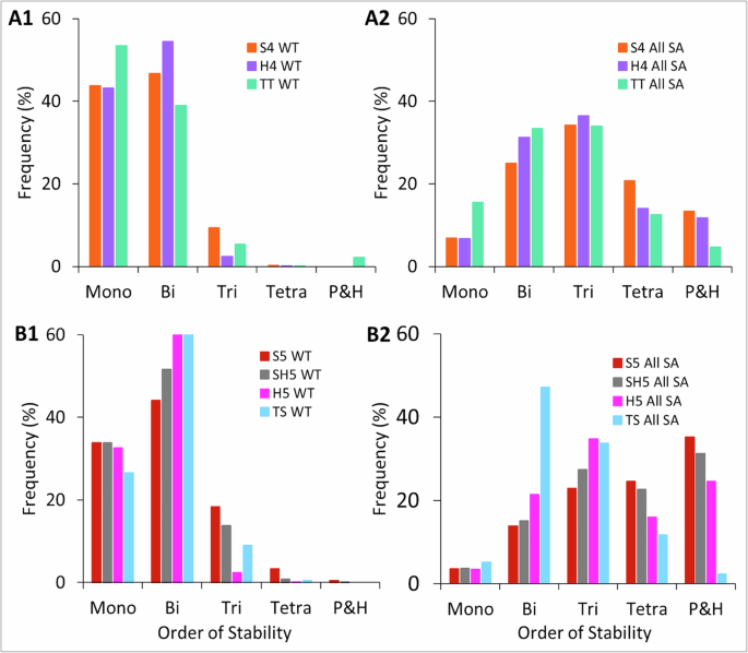
A1 Networks with three toggle switches have non-overlapping SSD. Despite having one node less than H4, cyclic network TT still shows some possibility for tristability. B1 Four-node networks again show non-overlapping higher-order SSD. Again TS, despite having one node less than H5, has greater tristable frequencies showing that cyclic network TS functions like a serial network by supporting higher-order steady-states. A2, B2 Self-activated counterparts of networks in (A1, B1).
Complete networks operate closer to serial and cyclic networks than hub networks
Complete graphs are defined as undirected graphs in which every pair of distinct vertices is connected by a unique edge. We derived a terminology from this and constructed complete toggle networks in which every pair of nodes is connected by a toggle switch. These networks resemble our hub networks, and therefore, we wanted to analyze and compare their steady-state dynamics with the serial, cyclic, and hub networks. We thus constructed eight complete toggle networks, C3 to C10. Firstly, we made a comparison of the steady-state distributions of small and large complete networks, which revealed that, among these complete networks, C3 (which represents a toggle triad network) has the highest number of monostable states and C10 has the lowest number of monostable states. With a continuous increase in network size, we find a constant reduction in the frequency of lower-order states and an increase in the frequency of higher-order states (Fig. 5A), which is a property of serial and cyclic networks. This analysis thus reveals a clear distinction between hub and complete networks by showing that though complete networks resemble more to hub networks topologically, however, they operate closer to serial and cyclic networks than hub networks.
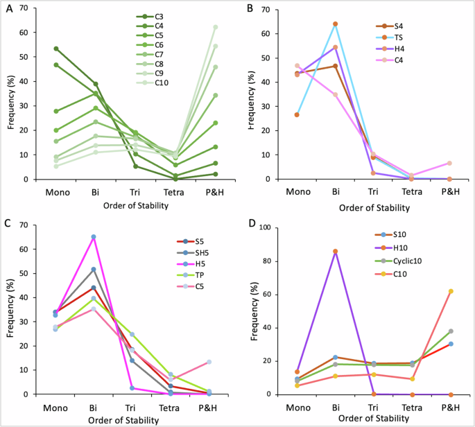
A Complete networks with three to ten nodes. B Comparison of a four-node complete network, C4, with all four-node networks. C Comparison of a five-node complete network, C5, with all five-node networks. D Comparison of a ten-node complete network, C10, with ten-node serial (S10), hub (H10), and cyclic (cyclic10), networks.
Next, we wanted to understand how same-size (in terms of node numbers) serial, hub, and cyclic networks perform compared to the equivalent-size complete networks. To investigate this, we performed a cross-comparison of four and five-node complete networks with all four and five-node serial, hub, and cyclic networks, respectively. Among the four-node serial, hub, cyclic, and complete networks, we observe that C4 exhibits a relatively lower probability of bistable states and the highest probability of penta-and higher-order (P&H) states. The mono, tri, and tetrastable frequencies are however comparable (Fig. 5B). Further, a comparison of the five-node serial, hub, and cyclic networks with a five-node complete network again shows a relatively lower probability of bistable states and a higher likelihood of P&H states in C5. The frequency of monostable states reduced while the tri- and tetrastable frequencies are comparable (Fig. 5C). Finally, we asked whether this trend could be maintained in large networks, leading us to compare steady-state distributions in ten-node serial, hub, and complete networks. In these networks, we observe that the C10 network has a relatively lower probability for mono, bi, tri, and tetrastable states and the highest likelihood for P&H states (Fig. 5D). The decrease in the lower-order state frequencies compensates for the constant increase in P&H states. While the difference between corresponding mono, bi, tri, and tetrastable states in serial/cyclic and complete networks is less (≈10%), the P&H state frequencies differ by around 30% (Fig. 5D). These findings show that, with an increase in the size of the complete network, the lower-order stability decreases and the higher-order stability increases. Overall, a cross-comparison with the corresponding serial, hub, and cyclic networks highlights that complete networks operate like serial and cyclic networks.
Perturbations to reduce network dynamics to lower-order stability: more negative feedback loops are more effective than less positive feedback loops
As discussed earlier, HDFLs as part of complex networks, drive cell fate transition during differentiation mechanisms and diseases such as EMT-induced non-genetic tumor heterogeneity and carcinoma metastasis. For instance, mutual repression between members of miR200 and ZEB gene families, represented by the S3 network, can drive a carcinoma cell to at least three phenotypes: mesenchymal fate (low miR200, high ZEB), hybrid epithelial-mesenchymal fate (medium miR200, medium ZEB), epithelial fate (high miR200, lowHT ZEB)30. Similarly, mutual repression between three genes, RORγT, GATA3 and T-bet, depicted by TT, can drive naive CD4 + T cell into three distinct states—Th1 (high T-bet, low GATA3, low RORγT), Th2 (low T-bet, high GATA3, low RORγT) Th17 (low T-bet, low GATA3, high RORγT)48. The fundamental component that recurs in all of these HDFLs is the PFL formed by two mutually antagonistic genes also called a toggle-switch. And, so far, we know that more toggle-switches connected serially (like in S5), result in numerous alternative states. We asked, can we target these PFLs to restrict the state space of these networks to a few states To identify such targets (gene interactions), we introduce two types of edge perturbations (Fig. 6) across the networks. The first is the “edge-deletion” (ED) perturbation, where we delete an edge, one at a time, between the nodes and repeat the process as long as the network remains intact. Each ED perturbation thus gradually reduces the number of PFLs in the network. In the “edge-sign-reversal” (ESR) perturbation, we change the sign of one of the inhibitory interactions between the two nodes to activation. Thus, unlike ED, each ESR perturbation converts a PFL into a negative feedback loop (NFL) so that more ESRs imply more negative feedback loops (Fig. 6). These two perturbations applied on any network with N edges will give rise to 2N perturbed networks. The implications of these edge perturbations have been tested in vivo. For instance, a recent study analyzed the impact of the disruption of the inhibition of miR200 by Zeb1 on the cellular dynamics of EMT and reported the loss of (hysteric) bistability with the occurrence of a biphasic (non-hysteric) cell transition in the mutant (perturbed) network50. Moreover, another closely relevant study has shown that disrupting the inhibition of Zeb1 by miR-200 is sufficient to drive the phenotypic transition of epithelial cancer cells to mesenchymal cancer cells, highlighting the importance of this interaction as a potential therapeutic target in tumor progression and invasion26.
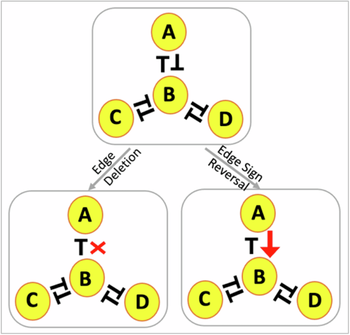
An unperturbed network (WT) with ED and ESR perturbations. In ED, one of the edges between the two nodes is deleted, resulting in a breakdown of the positive feedback loop. In ESR, the sign of one of the edges between the two nodes is changed from inhibition to activation so that a positive feedback loop transforms into a negative feedback loop. The lines with a bar denote inhibition/repression and those with an arrow denote activation.
We simulated these networks like before using RACIPE and compared the SSD of each perturbed network with its WT (unperturbed) counterpart. Our findings show that both ED and ESR perturbations reduce network SSD to lower-order stability. Particularly, a single ED or ESR increases the frequency of monostable states, which is compensated by a decrease in the frequency of higher-order stability (Fig. 7). This trend follows throughout the networks, and we observe that an ESR is more effective than ED, in the sense that each ESR increases more monostable solutions (by percentage) than an ED (Supplementary Fig. 4A1–C1, Supplementary Fig. 5D1–E1, Supplementary Fig. 6F1–H1). On the other hand, we observe that when all the genes (network nodes) are autoregulated, the same two perturbations have less effect on the SSD of the network (Supplementary Fig. 4A2–C2, Supplementary Fig. 5D2–E2, Supplementary Fig. 6F2–H2). This is evident from the expression data which shows that the number of feasible states (clusters) decrease with an ED or ESR in WT networks (Fig. 7C), which however remain unchanged in their self-activated counterparts (Fig. 7D). We thus conclude that ESR (which increases an NFL) and ED (which decreases a PFL) perturbations work only in non-autoregulated networks to reduce the network state space of the network. These edge perturbations can serve as inputs to future efforts focussing on in-depth understanding and controlling multiple cell lineages in differentiation and, importantly, in preventing phenotypic heterogeneity enabled during the EMT-induced metastasis of carcinomas.
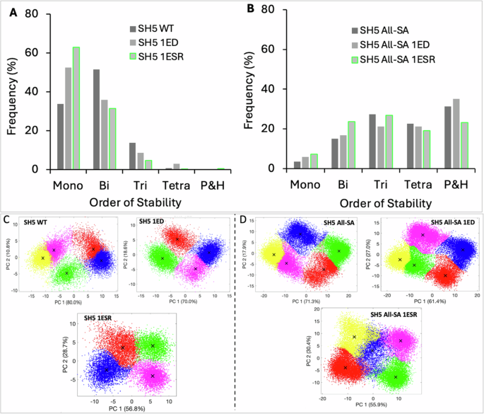
A In a non-autoregulated (without self-activations) network, an ESR increases monostable states more rapidly than an ED. B The effect of edge perturbations is diluted by the self-activations as the differences in SSD between WT and its two perturbed counterparts are negligible. Gene expression data of WT (C) and SA (D) networks projected on the 1st and 2nd principal component axis after clustering. Each cluster represents the steady state of a network state. SH5 WT means SH5 unperturbed network, 1ED means one edge detection, 1ESR means one edge sign reversal, and all-SA means all nodes are self-activated.
Identifying perturbations to convert multistable networks into monostable networks
In the previous section, we found that an ED or ESR increases the likelihood of lower-order stability. Taking, for instance, SH5 as a representative network, we show that for the SH5 (wild type) network bistable states are the most frequent (~50%), followed by monostable (~35%) and tristable (~15%) states. This implies that SH5 likely enables two cell states and in rare cases, three states (Fig. 8A). A single ED in SH5 results in a sharp increase in the frequency of monostable states (second bar in Fig. 7A) compensated by a decrease in bi-and tristable states. We wanted to analyze the effect of increasing edge perturbations on the dimension of state space and asked how many perturbations can turn the network dynamics into a single state. To analyze that, we gradually increased edge perturbations in the network and noted the SSD after each additional perturbation. We find that as EDs increase, the frequency of monostable states also increases linearly, while the frequency of bi-and tristable states decrease sharply (Fig. 7A). We also discover that three and four EDs, respectively, eliminate the chance of tristability and bistability, thereby turning SH5 a monostable (single state) network. This is also evident in the scatter plot of 10,000 steady states, all of which essentially represent a single state (Fig. 8D). Since each ED eliminates a PFL and the SH5 network has four PFLs, our data thus shows that the removal of all PFLs turns SH5 into a single state (monostable) network.
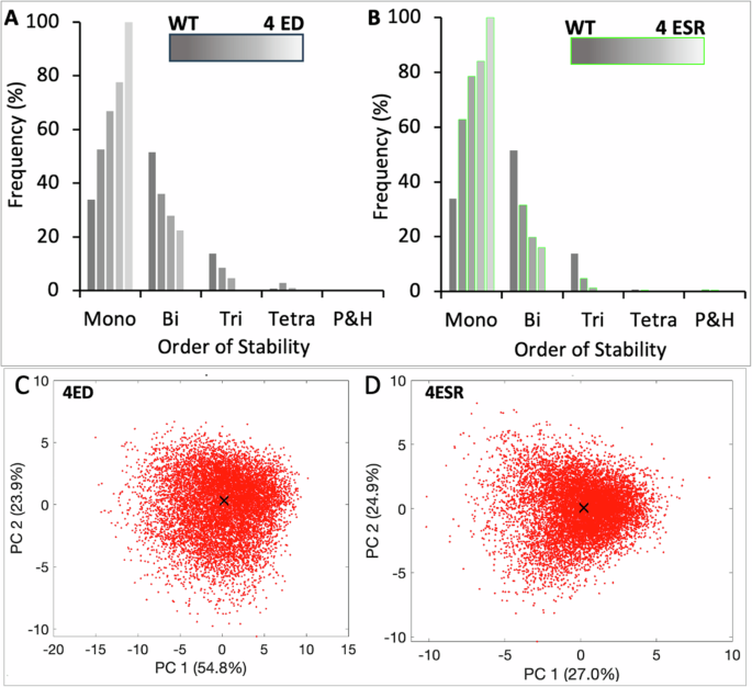
The plots illustrate the effect of increasing EDs and ESRs on the emergent SSD of HDFLs by considering SH5 as a representative network. A As EDs increase, the frequency of monostable states increases while bi-and-tri stable states decrease proportionately. Deleting three edges (breaking three PFLs) increases the frequency of monostable states to nearly 80% from nearly 30% in WT while also removing the chance of occurrence of any tristable solution. A completely monostable dynamics is achieved upon breaking all four PFLs in SH5. B As ESRs increase, network dynamics shift to mono-and-bistability faster than in the case of each ED. The 80:20 ratio of monostable: bistable states is achieved with two ESRs (i.e., converting two PFLs to NFLs) compared to three EDs and the frequency of tristable states is almost negligible. A completely monostable dynamics is achieved by converting four PFLs to NFLs. Gene expression data of SH5 with 4EDs (C) and 4ESR (D) projected on the 1st and 2nd principal component axis after clustering. A cluster represents a single state state. WT denotes no ED or ESR and 4ED (4ESR) denotes four edge deletions (edge sign reversals).
Next, we find that increasing ESRs also drive monostable states while reducing the frequency of higher-order stability (Fig. 8B). However, compared to EDs, the ESRs induce a rapid decline in bi-and tristable states and a surge in monostable states compared to ED. This is further supported by the fact that just two ESRs (as against three EDs) are required to eliminate tristable states in SH5 (Fig. 8B). However, four ESRs are required to attain a unique steady state (fifth bar in Fig. 7B shows 100% monostability) which also reflects from the scatter plot of the expression data in Fig. 8D. The single cluster observed in the scatter plot shows that all the 10,000 steady states in SH5 network with 4ESR essentially represent a single state. Our findings thus reveal that breaking all the (positive) feedback loops in a network converts a multistable network into a single-state network. This data is consistent with the traditional studies relating positive feedback loops with multistability.
The positive (negative) correlation between multistability and PFLs (NFLs) is observed across the HDFLs (Supplementary Fig. 7A1-H1). However, in their self-activated counterparts, perturbations shift the SSD peak to the left (lower-order stability), and with maximum perturbations, the peak settles around bi- and tristability (Supplementary Fig. 7A2-H2). This isn’t surprising, since we have previously shown such a correlation of multistability with PFLs and NFLs in large and complex EMT networks as well11. We thus conclude that regardless of the network size and topology, PFLs and NFLs have opposite effects on multistability: more PFLs favor higher-order stability while more NFLs enable lower-order stability. Our results, therefore, provide interesting insights into the association of topology with emergent multistability and can have clinical implications to decode the mechanism enabling multi-fate cell lineages and heterogeneity of carcinomas.
Position of edge perturbation has significance in networks with self-activated nodes
The HDFLs with autoregulated (self-activated) genes are more likely to exhibit multiple alternative states than those without autoregulations. One can then expect that the same perturbation can have a differential effect in auto- and non-autoregulated networks. To investigate this, we first tested our hypothesis on non-autoregulated HDFLs by considering S3 as a representative case. In this network, an ED or ESR is applied at two positions, P1 and P2, in a network. The perturbations at positions P1 and P2 can be EDs or ESRs in the two toggle switches on either side of the central node of the network. We simulated the two perturbed networks and compared the SSDs with their WT counterpart. Our data shows that EDs at both positions P1 and P2 (one at a time) result in similar SSD, implying that an ED at any position in a network will have the same effect (Fig. 9A). Next, we did the ESRs at the positions P1 and P2, one at a time. Strikingly, our data shows a complete overlap of two SSDs (Fig. 9B). We thus conclude that, in HDFLs without autoregulated genes, the same type of edge perturbation at two different positions creates the same impact and, therefore, the position of perturbation has no significance.
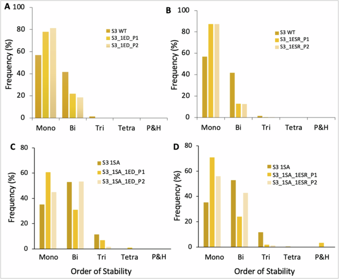
A A non-self-activated (WT) S3 network and its two ED perturbations. B Same as (A) but with ESRs. C S3 network with one of the terminal nodes self-activated and its two ED perturbations. (D) same as (C) but with ESRs. Perturbations, P1 and P2, are done in two toggle switches on the opposite sides of the central node of S3 so that in (C, D), P1 involves the SA node while P2 doesn’t. 1EDP1/1EDP2 (1ESRP1/1ESRP2) denote single-edge deletions (edge sign reversals) at P1 and P2 position. This terminology follows throughout the bar plots in Fig. S8.
To test our hypothesis on HDFLs with autoregulated nodes, we self-activated one of the terminal nodes of S3. With a self-activated node, the two PFLs on either side of the central node become “structurally” different. Here, the perturbation at position P1 refers to an ED or ESR between two nodes involving a self-activated node, while perturbation at position P2 refers to an ED or ESR in the other toggle switch that doesn’t have a self-activated node. We found that ED or ESR in the PFL involving the self-activated node (i.e., at P1 position) substantially increases (decreases) the likelihood of monostable (bistable) states than an edge perturbation in PFL without self-activated nodes (P2 position). As shown, EDs at P1 position increase nearly 25% monostable states and decrease nearly 20% bistable cases than an ED at position P2 (Fig. 9C). This effect persists when EDs are replaced by ESRs (Fig. 9D) and is also observed across HDFLs (Supplementary Fig. 8). Our findings thus highlight that in networks involving self-activated genes, disrupting the binding interactions between self-activated genes can be more effective in restricting the network dynamics to lower-order stability than disrupting the interactions between non-self-activated genes. These findings thus reveal crucial targets to, for instance, control cell fate transition in diseases such as restricting phenotypic heterogeneity in carcinomas.
Cell fate transition dynamics in serial, hub, and cyclic networks
We investigated fate (state or phenotype or lineage) transitions between the multiple phenotypes (or fates or states) observed in each network, we performed bifurcation analysis of the mathematical models corresponding to three serial networks, S3, S4, and S5, a hub network, H5, and a cyclic network, TP, for increasing basal production rate, ({B}_{1}), of gene ({x}_{1}). Increasing ({B}_{1}) reflects the fate induction signals (such as TGF-beta, SNAIL, etc.) from the extracellular environment that elevate the basal expression level of lineage-specifying transcription factor of gene ({x}_{1}). In each model, we analyzed the impact on the steady-state expression of node ({x}_{1}) subject to increasing ({B}_{1}) levels (Fig. 10).
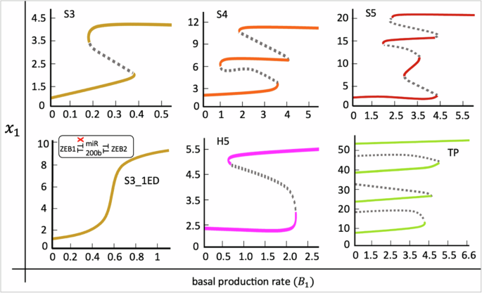
Top panel: three serial networks, S3, S4, and S5. Bottom panel: single edge deleted S3 network, hub network H5, and cyclic network, TP. Solid curves represent stable steady states, and dashed curves represent unstable steady states. In S3, S4, S5, and H5 networks, ({x}_{1}) represents ZEB1, GRHL, GRHL, and miR200, respectively. In TP network ({x}_{1}) represents node A. The colors of the stable branches of the bifurcation diagrams are matched to the color codes of the networks in Fig. 1. The model system (4) was used for the bifurcation analysis of S3, S4, and S5 networks. The model systems for H5 and TP networks and the parameters for all models are listed in Supplementary Information, Section S9. Bifurcations were generated using custom MATLAB codes.
In the S3 network, we observe that as ({B}_{1}) increases, ({x}_{1}) experiences a linear change until the saddle-node bifurcation threshold is crossed, after which ({x}_{1}) abruptly jumps to higher levels. The high levels of ({x}_{1}) represent the fate of ({x}_{1}) (ZEB1, in this case) while the low levels represent the fate of an antagonistic gene (miR200b, in this case). The transition is also reversible because we observe a high to low ({x}_{1}) transition as ({B}_{1}) is gradually reduced or withdrawn (Fig. 10, S3 network). The nonlinear process underlying the fate transitions is hysteresis, which suggests that cell fate transition is subject to signal induction and the history of the cell’s earlier commitments. In the S4 and S5 networks, we observe a multistep fate commitment program, where the preceding lineages vanish as ({B}_{1}) increases, and eventually, only the lineage ({x}_{1}) is retained (Fig. 10, S4 and S5 networks). A similar kind of multistep fate transition has also been observed in a relatively complex EMT network containing three serially connected toggle switches at its core51. This suggests that serially connected toggle switches might have evolved to be exploited by the cells to drive to multiple fates. Further, retention of lineage ({x}_{1}) in all models is expected, since a continuous induction of ({B}_{1}) introduces lineage bias, which overcomes the system dynamics, eventually steering to the biased fate. This observation suggests that fate bias can have implications in fate engineering and can be utilized to steer cells to the desired fates.
Next, we asked whether the double-negative (positive) feedback loops can have roles other than ensuring multistability in the networks. To investigate this, we performed an edge deletion perturbation in the S3 network, which resulted in the removal of the inhibitory effect of miR200b from ZEB1. As the perturbed network was subject to ({B}_{1}) induction, we observe that the hysteresis mechanism (that governed fate transitions in the S3 network) is lost in the perturbed S3 network where cell fate transition is now regulated by a (non-hysteric) biphasic mechanism (Fig. 10, S3_1ED network). This finding corroborates a recent experimental study showing that in vivo disruption of the inhibition of miR200 by Zeb1 in a dual-negative ZEB1–miR200 feedback loop resulted in the loss of hysteric mechanism of cell fate transition and the mutant cells switch to the alternative fates through a (non-hysteric) biphasic transition50. This finding, therefore, reveals an additional role of tightly balanced positive feedback loops in enabling cell transition dynamics in a discrete, switch-like manner, which is reported to have significance in enhancing lung metastatic colonization efficiency50.
Among the hub networks, we analyzed fate transition in a five-node hub network, H5, which, as per our earlier observations, exhibits two states for a wide range of parameter sets (Fig. 2C, H5 network). Our bifurcation analysis is consistent with our previous observations, showing a reversible transition between two fates (low to high ({x}_{1}) and high to low ({x}_{1})) (Fig. 10, H5 network). A comparison with the bifurcation diagram of the S3 network shows that the H5 network exhibits bistability for a relatively wide range of ({B}_{1}). This suggests that compared to the serial topology, hub-type topology might be dedicated to a robust transition between the two fates, often called as robust bistability. Finally, among the cyclic networks, we analyzed the five-node network, toggle polygon (TP). The bifurcation diagram shows a remarkably robust multistep commitment subject to ({B}_{1}) induction (Fig. 10, TP network). However, the commitment to each stage has restricted reversibility since the withdrawal of the signal does not revert cells to earlier states. An interesting aspect of irreversible fate commitments is that once the cell acquires a certain lineage, the transition to other lineages is eliminated when the signal is abolished. This observation is consistent with the multistep irreversible fate transitions observed during the early T-cell development34.
Collectively, these findings suggest that different network topologies enriched in complex gene networks might be dedicated for a specific order of stability, and their conjunction might suffice for establishing a robust cell fate transition program.
Discussion
Different network structures with specific dynamical behavior underlie various cell fate decision-making programs, including epithelial-mesenchymal plasticity. Among these, positive and negative feedback loops are ubiquitous and widely studied network motifs with well-known functionality. However, the dynamics of PFLs interconnected through distinct topologies remain unexplored. Here, we identify three families of interconnected PFLs (HDFLs) in complex transcriptional networks driving EMT-induced cell fate transition during metastasis and CD4 + T cell lineage decision. We demonstrate that HDFLs containing nodes of higher centrality (such as hub networks) have restricted attractor space, while those with lower node centrality (such as serial and cyclic networks) give rise to higher dimensional attractor space. We found that these results also hold in larger (10 node) “synthetic” serial and hub networks, thereby establishing that less (more) connectivity between toggle switches in the networks results in a higher (lower) number of stable states (phenotypes). This is in contrast to “random” gene networks in which neither gene number nor connectivity increases the number of steady states, as shown by Mochizuki A. (2005)52.
To rule out the possibility that our conclusions are sensitive to the numerical integration scheme and the bounds of parameters, we used an alternative integration scheme and found that our results remain unchanged (Supplementary Fig. 9). Furthermore, we rule out the possibility that our results are the artifact of parameter bias by showing a striking similarity in state frequency distributions obtained from Boolean (see Methods) and RACIPE modeling approaches (Supplementary Fig. 10). From the evolutionary point of view, these findings suggest that different families of HDFLs have selectively evolved and become fundamental to cell fate transition programs that drive cells to multiple different fates. In the context of EMT-induced cell fate transition, these results highlight that interconnected positive feedback loops with less node centrality can be the most crucial gene network structures to drive cells to different fates along the E-M phenotypic spectrum leading to non-genetic phenotypic heterogeneity in carcinomas.
Next, we were interested in identifying crucial targets to reduce higher-order network dynamics to lower-order dynamics. We perturbed networks with EDs (breaking PFLs) and ESRs (introducing NFLs) and compared the SSD of perturbed networks with their “WT” counterparts. While EDs and ESRs both reduce the order of stability, the effect of ESRs is found to be more pronounced than EDs. Through bifurcations, we analyzed cell fate transition dynamics and found that extracellular fate-inducing signals can drive cells in a step-wise, discrete manner to different fates. We also found that breaking specific feedback loops can alter the mechanism of cell fate transition where cells can continuously transition to alternate fates, thereby identifying the roles of positive feedback loops beyond multistability. Further, we investigated the significance of the position of perturbation in networks with and without self-activated genes. Our analysis revealed that, in networks without self-activated genes, the position of edge perturbation doesn’t have any major significance as ED or ESR at any position results in overlapping SSDs of the network. However, strikingly, in networks with self-activated genes, an edge perturbation in the feedback loop involving a self-activated gene drastically reduces network dynamics to lower-order stability than an edge perturbation in the feedback loop between two non-self-activated genes. Further, the effect is more pronounced due to ESRs compared to EDs. This finding identifies precise gene interaction targets to prevent cells from diverging to multiple fates. In the context of EMT, this finding can serve as a potential input to experimental biologists to identify inhibitors of EMT-enabled non-genetic phenotypic heterogeneity and metastasis of carcinoma.
Our results conveniently disentangle the operating principles of three families of interconnected PFLs by shedding light on the intricacies of gene numbers, connectivity (topology), and their implications on the number of stable states. These findings can have crucial implications in comprehending cell fate transitions in development and disease. Since these networks form the foundation of complex networks underlying cell fate transitions, future work should investigate whether the dynamics of these network motifs withstand the complexity of the large “parent” networks. This investigation can reveal the principles enabling multistability in complex regulatory networks. Moreover, given the crucial role of noise in fate transition, it would be interesting to analyze cell fate transition dynamics in these networks under the noise-driven (stochastic) mode as against the signal-driven (continuous) mode analyzed in this study. A rigorous analysis of these aspects can provide a blueprint for the design of robust synthetic multistable circuits that can be employed to engineer, control, and alter the cell fate transition programs.
Methods
Mathematical model (Continuous)
Traditionally, interactions between nodes in a network are encoded in a directed graph, (G=(V,E)) on (N) vertices (V={1,,2,ldots ,{N}}). Suppose that we have an (N)-node network with dynamics of the form (dot{{x}_{k}}) = ({B}_{k}), where (x=left({x}_{1},,{x}_{2},,ldots ,,{x}_{k}right){{in }}{{mathbb{R}}}^{k}) is the state vector, and ({B}_{k}) describes the evolution of the node ({x}_{k}) in the absence of any regulatory interactions in the network and is referred to as the basal production rate or leakage rate. Suppose the function H represents the influence of the joint state of (i) number of nodes on node (k) in G. Assuming the interactions are multiplicative (though these can be defined to be additive also), the tuple ((G,{B},{H})) defines a dynamical system on a network through the following coupled system of differential equations,
Here, (dot{{x}_{k}}) represents the time-derivative of ({x}_{k}) and ({P}_{{k}}) is the first order maximum production rate of node k under the control of the (i) interacting nodes. In gene regulatory networks, the function (H) can be either activatory or inhibitory. We use a unified function, ({H}_{sh{ift}}), to model both activatory and inhibitory interactions. For a particular node ({x}_{i}), this shifted Hill function is defined as follows,
where ({x}_{0}) represents the activation/inhibition threshold, ({n}_{{x}_{i}}) the Hill coefficient, and (lambda) the fold change in activation/inhibition. Depending on the value of (lambda), ({H}_{sh{ift}}) can either be monotonically increasing (activatory) or decreasing (inhibitory) as denoted below,
Using (2) in (1), we get system (3), modeling the evolution of a k-node network,
where the degradation rate, (d), is of zero order.
Using the above modeling formalism, the system (3b) describes the dynamics of the S5 network, where ({{x}}_{k}), (k=1,,2,,3,,4,,5) represents GRHL, ZEB2, miR200b, ZEB1, and miR200c, respectively. The model systems for other networks can be obtained similarly. However, one can immediately deduce model systems for S3 and S4 networks from the model system (4).
Here, ({x}_{{AB}}) denotes the threshold of gene B repressing gene A, ({n}_{{AB}}) denotes the cooperativity of gene B repressing gene A, and ({lambda }_{{AB}}) denotes the fold-change in the expression of gene B due to gene A.
Numerical simulations
The numerical simulations are performed in RAndom CIrcuit PErturbation (RACIPE) https://github.com/simonhb1990/RACIPE-1.043. We used the Euler method of integration with a step size of 0.1, 100 initial conditions, and 20 iterations for each initial condition. The cut-off for convergence of steady state (time-invariant solution) is fixed at 1.0. The results, however, remain unchanged upon concurrently reducing the step size by 100-fold, increasing the number of initial conditions and iterations by 10-fold and 5-fold, respectively, or changing the integration scheme to RK45 (Runge-Kutta method of order 5/4). Also, the results remain invariant when the maximum production and degradation rates of the molecules are increased by 10-fold (Supplementary Information, Section S7). Simulation of all the networks is done in triplicates, with each replicate having 10,000 parameter sets, which takes into account cell-to-cell heterogeneity in biochemical reaction rates. These parameters are randomly sampled from reasonable, predefined ranges listed in Table 1 using log-uniform distribution. For each network, the output is a data set in which columns correspond to genes, and the rows correspond to the stable steady states. This data takes a form similar to typical microarray data, and we employ clustering techniques (discussed below) to identify the total number of feasible states allowed by a network.
Mathematical model (Discrete)
The Boolean modeling approach is a discrete, logic-based mathematical technique to analyze the dynamics of biological networks53,54. The state of the network is defined by a string of binary variables ({{S}_{i}}), determining if each node (gene) is expressed (left({S}_{i}=1right)) or not (left({S}_{i}=0right)). Interactions between two nodes (i) and (j) are defined in a matrix ({J}_{{ij}}) defined as
A simple majority rule governs the asynchronous, discrete time evolution of a network of N nodes, setting each node to ({S}_{i}=1) if the sum of its promoting contacts exceeds the sum of its inhibitory interactions and ({S}_{i}=0) otherwise. When there are ties, the node remains in its current state without being modified. This evolution rule is formally expressed by the following master equation,
It should be noted that this model does not include any kinetic constants, and the only input to the formalism is a set of (10,000 in our case) randomly sampled initial conditions. Its entire foundation is the network’s ‘wiring’ diagram, which is determined by the interaction links ({J}_{{ij}}) and their sign (+1/{-}1). Accordingly, the predictive ability of the Boolean model does not depend on precise quantitative estimates of concentrations and timings. It rather offers a panoramic perspective of the entire range of potential network states.
Comparison of RACIPE and Boolean simulations
To compare the outputs of RACIPE and Boolean models, we constructed a mapping that transforms the continuous variable into a discrete (Boolean) variable using the following equation,
where the mean ((mu)) and the standard deviation ((sigma)) are taken over all the 10,000 models.
The transformation happens in the following three steps:
-
(i)
Performed p/d normalization of each steady state (SS) to account for extremes in sampling of the production ((p)) and degradation ((d)) rate parameters. Here, each SS was divided by the ratio of production and degradation rate obtained from the corresponding parameter set.
-
(ii)
The normalized expression levels of all steady states are then converted into Z-scores by scaling about their combined mean.
-
(iii)
The states are then classified into 1 (high) and 0 (low) depending on whether the Z-score is positive and negative, respectively.
Next, we calculated the frequency of a particular SS by counting its occurrence across all parameter sets (10,000 in our case). In Boolean simulations, every network is run for 10,000 initial conditions, and the frequency of steady states is obtained by counting their occurrence across all initial conditions. Finally, the frequencies of overlapped states give us a fair comparison of the outputs of the two simulation procedures. To quantify the similarity between the two steady-state frequency distributions obtained for a particular network, we use Jensen-Shanon divergence (JSD). JSD is a symmetric form of Kullback-Leibler divergence (KLD).
where (A) and (B) are the two distributions defined on the sample space ({mathscr{X}}), (M=frac{1}{2}(A+B)), and the KLD is defined below
The ({JSD}in [0,,1]), with distributions becoming more similar as ({JSD}) tends to (0) and with identical distributions at ({JSD}=0.)
Data clustering and projection
Principal Component Analysis (PCA)
The PCA was used to project the Z-score normalized data on the two principal axes, explaining the maximum percentage of the total data variance. We used singular value decomposition to perform PCA.
K-means Clustering
We used K-means clustering, an unsupervised learning algorithm, with L1 norm (defined below) to segregate the data into different clusters and identify the feasible alternate states.
for (X=,left({x}_{1},,{x}_{2},,{x}_{3},,ldots ,,{x}_{n}right)) and (Y=,({y}_{1},,{y}_{2},,{y}_{3},,ldots ,,{y}_{n}))
To ensure that the clusters identified by the algorithm were correct, the algorithm was run 10,000 times for each data set. The best clustering outcome was chosen to be the one with a minimum value of Within Cluster Sum of Squares (WCSS) defined below
where the first two summations calculate distances of data points in a cluster from the centroid C of that cluster, and the third summation takes the sum over all clusters.
Responses