Robust parameter estimation and identifiability analysis with hybrid neural ordinary differential equations in computational biology
Introduction
Mathematical and computational models are increasingly employed in the study of biological systems1. These models not only facilitate the creation of predictive and explanatory tools2 but also offer a means to understand the interactions among the variables of the system3.
The well-established approach to develop a mathematical model for biological systems, i.e., the mechanistic modeling approach4, relies on encoding known biological mechanisms into systems of partial or ordinary differential equations (PDE or ODE) using suitable kinetic laws, e.g., the law of mass action or Michaelis-Menten kinetics5. These equations typically incorporate several unknown model parameters, making parameter estimation a central challenge in model development6. The prevailing approach to parameter estimation involves optimizing the model dynamics to align with experimental data7. Various optimization techniques are employed for this purpose, including linear and nonlinear least squares methods8,9, genetic and evolutionary algorithms7, Bayesian Optimization10,11, control theory-derived approaches12 and, more recently, physics-informed neural networks6. The scarcity of experimental data and the measurement noise often lead to non-identifiability issues, where the optimization problem lacks a unique solution13. To address this challenge, various methods exist to analyze the identifiability of model parameters. Structural identifiability analysis14, performed before parameter estimation, analyzes the structure of the model to determine if parameters can be uniquely estimated. On the other hand, practical identifiability analysis15, conducted after parameter estimation, evaluates how uncertainties in experimental measurements affect parameter estimation.
Developing mathematical models and estimating model parameters with the mechanistic modeling approach presents significant challenges due to the need for a detailed understanding of the interactions between (and within) biological systems. Complex biological systems often involve processes at different scales, such as genetic, molecular, tissue, organ, or whole-body, and such intricate mechanistic details are only partially known16,17. To overcome the limits of mechanistic modeling, hybrid models that combine mechanistic ODE-based dynamics with neural network components have grown in popularity in various scientific domains18,19. The integration between neural networks and ODE systems is known by different names, such as Hybrid Neural Ordinary Differential Equations (HNODEs)20, graybox modeling21,22, or universal differential equations23. In a HNODE, neural networks are used as universal approximators to represent unknown portions of the system. Mathematically, HNODE can be formulated as the following ODE:
where NN denotes the neural network component of the model, f encodes the mechanistic knowledge of the system, and θ represents a vector of unknown mechanistic parameters. This approach has proven successful in several fields, and early results in isolated and relatively simple scenarios have shown promise in computational biology as well24,25. However, modeling with HNODEs remains an active area of research, and best practices for estimating mechanistic parameters and assessing their identifiability within this framework remain to be outlined.
Mechanistic parameter estimation within the HNODE framework presents significant challenges. Firstly, while model calibration in mechanistic models usually relies on global optimization techniques to explore the parameter search space9, training HNODE models necessitates the use of local and gradient-based methods23. Secondly, incorporating a universal approximator, such as a neural network, into a dynamical model may compromise the identifiability of the HNODE mechanistic components26,27. In this sense, the existing literature has focused on trying to enforce the identifiability of the mechanistic parameters within a HNODE by integrating a regularization term into the cost function28. Common choices for this regularization term include minimizing the impact of the neural network on the model28 or ensuring that the outputs of the neural network and mechanistic part are uncorrelated26. However, these approaches do not always guarantee the correct identification of the mechanistic part, and the outcomes depend on the specific regularization term used26. To the best of our knowledge, the identifiability analysis of the mechanistic parameters in a HNODE model has not been investigated in the literature so far.
In this contribution, we present an end-to-end approach for mechanistic parameter estimation and identifiability analysis in scenarios where mechanistic knowledge about the system is incomplete. Initially, we focus on tuning hyperparameters to embed our incomplete mechanistic model into a HNODE model that is capable of effectively capturing the experimental dynamics. Subsequently, we proceed to compute mechanistic parameter estimates by training the HNODE model. Following parameter estimation, we extend a well-established approach for mechanistic models to assess the parameter identifiability a posteriori. For identifiable parameters, we finally estimate asymptotic confidence intervals (CIs).
The proposed approach has been tested in three different in silico scenarios, that have been constructed by assuming a lack of information about some portions of known mechanistic models. We aimed to replicate typical conditions found in real-world scenarios, with a noisy and scattered training set describing the time evolution of a subset of the model variables. Firstly, we consider the traditional Lotka-Volterra model for predator-prey interactions. Despite being a relatively simple model, it shows the ability of the approach to identify compensations between the neural network and the mechanistic component of the HNODE model. Secondly, we evaluate the performances of our approach on a model for cell apoptosis29, known for the non-identifiability of part of its parameters. Thirdly, we consider a model of oscillations in yeast glycolysis30, which has been frequently employed as a benchmark for inference in computational systems biology due to its nonlinear oscillatory dynamics.
Results
A schematic representation of the workflow is presented in Fig. 1. The input of the pipeline consists of an incomplete mechanistic model containing parameters to be estimated, along with a time series dataset containing experimental observations of some of the system variables. By embedding the incomplete model into a HNODE model, our approach enables parameter estimation and identifiability analysis.
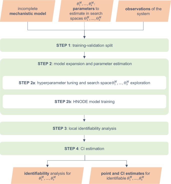
In the workflow schema, ({theta }_{1}^{M},ldots ,{theta }_{s}^{M}) denote the mechanistic parameters to estimate in the corresponding search spaces ({Theta }_{1}^{M},ldots ,{Theta }_{s}^{M}). HNODE: Hybrid Neural Ordinary Differential Equation, CI: Confidence Interval.
The workflow starts by splitting the observation time points into training and validation sets (Step 1). In the second step, using this partition, we expand the incomplete mechanistic model into a HNODE model. We employ Bayesian Optimization to simultaneously tune the model hyperparameters and explore the mechanistic parameter search space (Step 2a). The model is then fully trained (Step 2b), yielding mechanistic parameter estimates. In the next step (Step 3), we assess the local identifiability at-a-point of the parameters. For the locally identifiable ones, we proceed to estimate confidence intervals (Step 4).
In the rest of the section, we use the following notation. Let ({bf{y}}(t,{{boldsymbol{theta }}}^{M},{{boldsymbol{theta }}}^{NN},{{bf{y}}}_{{bf{0}}})in {{mathbb{R}}}^{n}), with (nin {{mathbb{N}}}^{+}), be the HNODE model defined by the following differential equation:
where ({{bf{y}}}_{{bf{0}}}in {{mathbb{R}}}^{n}) stands for the initial conditions, fM and ({{boldsymbol{theta }}}^{M}=({theta }_{1}^{M},ldots ,{theta }_{s}^{M})) denote the mechanistic part of the model and the (sin {{mathbb{N}}}^{+}) mechanistic parameters to be estimated, respectively, while θNN represents the neural network parameters. We denote the i-th component of the model as yi(t, θM, θNN, y0), with i = 1, …, n. Typically, only a subset of the system variables is observable; we indicate this subset with O ⊆ {1, …, n}. We assume to have access to the experimental measurements of the observable variables at m + 1 time points t0, …, tm; ({hat{y}}_{j}^{i}pm {hat{sigma }}_{j}^{i}) indicates the observations of the i-th variable at time tj, with the uncertainty reflecting the variability of the measurement. Additionally, we assume to have access to the initial conditions ({hat{y}}_{0}^{i}pm {hat{sigma }}_{0}^{i}) of all the variables.
The remainder of this section is organized as follows. First, we present a detailed description of each step in the workflow. In the subsequent subsections, we analyze the results of the pipeline across various in silico test cases. The implementation details and algorithmic setup for these test cases are outlined in the Methods Section. Given that the training of HNODE extends the techniques used for Neural Ordinary Differential Equations (NODE)31, we begin with an overview of the methods employed for training NODE, which precedes the description of the pipeline.
Background: NODE training
In this section, to discuss the NODE case, we assume that fM = 0 in Eq. (2), indicating no mechanistic knowledge about the system. Under this hypothesis, the vector field is entirely parameterized by the neural network NN, and the ODE:
represents a NODE. Given a loss function ({mathcal{L}}), the training of the NODE can be achieved through the minimization of the cost function:
where yi is computed numerically by integrating Eq. (3). Minimizing C(θNN) requires to back-propagate the error through the ODE solver algorithm used for the numerical integration of y. By the chain rule, for a differentiable ({mathcal{L}}), this amounts to compute the gradients
Chen et al.31 demonstrated that these gradients can be efficiently computed using adjoint sensitivity32,33, treating the ODE solver as a black box. Adjoint sensitivity requires a backward integration of the system and different numerical methods have been proposed to efficiently calculate it23.
As in the traditional ODE case, stiffness constitutes a significant challenge in the training of NODE34. However, as shown by Kim et al.35, there are specific ways to overcome this issue. These include employing deep neural network architectures, ad hoc methods for computing adjoint sensitivity, and a normalized loss function.
Step 1: training-validation split
In the first step of the workflow, the observation time points are divided into training and validation sets, indicated with ({{{t}_{j}}}_{jin T}) and ({{{t}_{j}}}_{jin V}) respectively. The validation time points are chosen from t1, …, tm to ensure a homogeneous distribution along the observed trajectory.
Step 2: model expansion and parameter estimation
In this step, the incompletely specified mechanistic model is expanded into a HNODE model through the use of neural networks to replace unknown portions of the system. The estimates for mechanistic parameters are derived by training the HNODE model.
The training of a HNODE model is analogous to that of NODE. Adopting a loss function ({mathcal{L}}), the most straightforward approach would be minimizing the cost function:
Here, ∣T∣ and ∣O∣ denote the cardinality of T and O respectively. Gradients of C(θM, θNN) with respect to mechanistic and neural network parameters are calculated via adjoint sensitivity methods. If the cost function defined by Eq. (5) is employed, a single trajectory of y spanning from t0 to tm is computed at each epoch of the training. This approach, known as single shooting, is often suboptimal due to the potential risks of the training getting stuck in local minima27.
Therefore, we adopt the multiple shooting technique (MS)36. In MS, the time interval (t0, tm) is partitioned into different segments. Rather than computing a single trajectory of y on the entire training interval, a potentially discontinuous trajectory yPW(t, θM, θNN) is reconstructed piece-wise by solving an initial value problem on each segment, adding the states of the system at the initial points of each segment as additional parameters to be optimized. The cost function is then composed of two terms:
In Eq. (6), CFIT measures the difference between the piecewise-defined trajectory and the training data, CDIS measures the discontinuity of the trajectory, and (rho in {mathbb{R}}) is a hyperparameter. For CFIT, we use the cost function defined in Eq. (5), adopting the loss function
in which the quadratic loss is weighted for the uncertainty measure if it is not zero. CDIS is computed by summing the squared values of the discontinuities at the extremes of the training interval partition. To prevent overfitting, in the case of noisy training data, we add an L2 regularization term. Given this cost function, the training is performed with a gradient-based optimizer, and gradients are computed using adjoint sensitivity methods. In our test cases, we use the Adam optimizer37, and we refine the results with L-BFGS38 on training datasets without noise.
To define the segmentation of the time interval, we partition the training set of time points into subsets containing the same number k of items (excluding the last interval), where k is a hyperparameter. When using MS to train the model, we introduce as additional parameters to optimize the state of the system at the initial points of each segment. These parameters are initialized with the measured states of the system at the time point when the corresponding system variable is observable; otherwise, they are initialized with the initial state of the variable.
How to tune the hyperparameters and explore the parameter search space
The hyperparameters requiring tuning can be grouped into three different macro-categories: the hyperparameters of the architecture of the neural network, the starting values of the mechanistic parameters to initiate the gradient-based optimization, and the hyperparameters related to the MS training. This latter category includes the segmentation of the time interval (t0, tm) used to define the piecewise trajectory, the weight factor ρ used in Eq. (6), the weight λ of the L2 regularization term, and the learning rate of the gradient-based method. Incorporating the initial values of ({theta }_{1}^{M},ldots ,{theta }_{s}^{M}) into hyperparameter tuning enables the integration of local gradient-based search with Bayesian Optimization techniques, as proposed by Gao et al.39 The objective is to globally explore the mechanistic parameter search space during this step.
The hyperparameters are tuned in two stages, described below.
Hyperparameter tuning – Stage 1
We simultaneously tune all hyperparameters, except for the L2 regularization factor λ, using the multivariate Tree-Structured Parzen Estimator (TPE)40,41. In each TPE trial, the HNODE model is trained for a limited number of MS iterations. The optimization metric during the TPE algorithm is the mean squared error on the validation time points of the trajectory predicted by the trained model:
As before, we employ a pure quadratic error when uncertainty indications on measurements are absent.
Hyperparameter tuning – Stage 2
In the second stage, we fix the hyperparameters tuned in the first step and focus on tuning the L2 regularization factor, λ, using a grid-search approach. In each trial during this step, the HNODE model is trained for an extended number of MS iterations, and we continue to employ the same metric as in the previous step to evaluate each trial.
The decision to split the tuning process into two stages is motivated by the observation that the effects of overfitting may not become apparent with a low number of iterations. Therefore, tuning λ in the initial stage might not be as effective. Conversely, conducting a large number of MS iterations in the first stage would significantly increase computational costs.
How to deal with stiffness
Before starting the hyperparameter tuning phase, the behavior of the HNODE model, whether stiff or non-stiff, is unknown. To train a stiff HNODE model, we follow the guidelines outlined for stiff NODE. This involves employing specialized techniques such as ad hoc adjoint sensitivity methods, deeper neural network architectures, stiff ODE solvers, and normalized loss functions. We do not include all configurations used for stiff systems as hyperparameters to tune, to prevent an excessive increase in the search space dimension. Instead, we propose initiating the hyperparameter tuning with non-stiff configurations and monitoring the integration of the HNODE model during the first trials of the process, such as observing the number of steps taken by the ODE solver to complete system integration. If stiffness is detected, we finalize the tuning process and we train the HNODE model using stiff configurations.
Step 3: local identifiability analysis
In this step, we investigate a posteriori the local identifiability of the mechanistic parameters ({theta }_{1}^{M},ldots ,{theta }_{s}^{M}) estimated with the model training. This is particularly important in HNODE models, as incorporating a universal approximator, such as a neural network, into a dynamical model may compromise the identifiability of mechanistic parameters. The following subsections introduce the foundational concepts for our approach and the description of the workflow.
Local identifiability at-a-point and sloppy directions
We refer to the combined neural network and mechanistic parameter estimates, obtained through the training in Step 2, as the single vector:
We recall that the k-th parameter of the model is locally identifiable at-a-point42 in (overline{{boldsymbol{theta }}}) if
implies ({theta }_{k}={overline{theta }}_{k}) for all θ in a suitable neighborhood of (overline{{boldsymbol{theta }}}) (for a discussion of the relationship between this and other definitions of parameter identifiability, we refer to Supplementary Note 1).
To study the local identifiability, we quantify the change in the HNODE model behavior, as parameters θ vary from (overline{{boldsymbol{theta }}}), with the function:
where ({gamma }_{i}=ma{x}_{j}{| {y}^{i}({t}_{j},overline{{boldsymbol{theta }}},{{bf{y}}}_{{bf{0}}})| }) is introduced to normalize the contribution to χ of each variable. In a neighborhood of (overline{{boldsymbol{theta }}}), the function χ can be approximated as:
where ({H}_{chi }(overline{{boldsymbol{theta }}})) denotes the Hessian matrix of χ in (overline{{boldsymbol{theta }}}). If v is an eigenvector of ({H}_{chi }(overline{{boldsymbol{theta }}})) and μ is the corresponding eigenvalue, for small values of α it holds:
Eq. (9) implies that the HNODE model behavior does not change significantly when the parameters move along the direction identified by v if μ is zero. In mechanistic models, the eigenvectors related to zero or almost-zero eigenvalues are commonly called sloppy directions43,44,45. Denoting with V0 the null space of Hχ, spanned by the eigenvectors related to zero eigenvalues, and with VS the subspace spanned by the remaining eigenvectors, each parameter θk of the model can be decomposed as:
where π0(θk) and πS(θk) denote the projection of θk onto V0 and VS respectively. π0(θk) represents the local direction that maximizes the parameter perturbation without affecting the model behavior. Although one might expect identifiability of θk to yield ∥π0(θk)∥2 = 0 and ∥πS(θk)∥2 = 1, strict equalities generally do not hold. This is because, as observed by Gutenkunst et al.43, each sloppy eigenvector typically encompasses mixed components of nearly all model parameters. Hence, 0 < ∥π0(θk)∥2 < 1 applies to all model parameters.
How to assess the local identifiability at-a-point
Our approach involves identifying mechanistic parameters ({theta }_{1}^{M},ldots ,{theta }_{s}^{M}) having a significant projection onto the null subspace of the HNODE model. We proceed as follows. First, we compute ({H}_{chi }(overline{{boldsymbol{theta }}})) with the Gauss-Newton method:
In Eq. (10), we rescale the sensitivity coefficients to make them independent of the absolute values of the parameters46; this consideration is important when simultaneously considering both neural network and mechanistic parameters. ({H}_{chi }(overline{{boldsymbol{theta }}})) is a symmetric and positive semi-definite matrix. We proceed to determine the null subspace of ({H}_{chi }(overline{{boldsymbol{theta }}})) spanned by all eigenvectors corresponding to eigenvalues μ ≤ ϵ. Here, ϵ is a hyperparameter embodying the threshold used to distinguish zero eigenvalues in a numerical environment. To discriminate whether there exists a direction in the parameter search space along which we can significantly perturb the parameter ({theta }_{i}^{M}) without affecting the model simulation, we analyze the norm of the projection of ({theta }_{i}^{M}) onto V0. If it exceeds a predefined threshold δ, which is a second hyperparameter of our approach, we classify the parameter as non-identifiable.
Step 4: CI estimation
In the final step of our pipeline, we estimate CIs for the locally identifiable parameters. Several methods for estimating parameter CIs in mechanistic models have been proposed. We employ the Fisher Information Matrix (FIM)-based approach47. We assume that our observed data follow independent Gaussian distributions (N({y}_{j}^{i},{sigma }_{j}^{i})), and that our parameter estimator is an approximation of the maximum likelihood estimator, as proposed in Yazdani et al.6. Therefore, we can approximate the observed FIM as:
The pseudo-inverse of the FIM provides a lower bound for the covariance matrix of our estimators48. Consequently, we can define a lower bound ({overline{sigma }}_{i}^{M}) for the standard deviation of the estimator of the parameter ({theta }_{i}^{M}) by taking the square roots of the elements on the diagonal of FIM−1. We can then compute the lower bound for the α-level confidence intervals of ({theta }_{i}^{M}) as:
where Φx represents the x quantile of a standard Gaussian distribution.
Lotka-Volterra test case
In this section, we analyze the performance of the pipeline using a test case based on the Lotka-Volterra predator-prey model, which describes the temporal dynamics between two species, where one preys upon the other49. Although it is based on a relatively simple system, this test case offers the opportunity to evaluate the effectiveness of our approach in detecting compensations between the neural network and the mechanistic parameters of the model. Additionally, it allows for a discussion on why we opt not to enforce the identifiability of the mechanistic parameters through the use of a regularizer in the cost function, as proposed by Yin et al.28.
The full mechanistic model is defined by the following system of ODE:
where y1 represents the prey population, and y2 represents the predator population. In this context, we assume a lack of information regarding the interaction terms between the two species (βy1y2 and γy1y2). By replacing them with a neural network (NN:{{mathbb{R}}}^{2}to {{mathbb{R}}}^{2}), we have the following HNODE model:
Our objective is to estimate and assess the identifiability of the prey birth rate α, assuming we know the predator decay rate δ. To generate in silico the observation datasets, we numerically integrate Eq. (12) over the interval from t = 0 to t = 5 years (the initial conditions and parameters are provided in Supplementary Note 2) and sample the states every 0.25 years (resulting in 21 observed time points). We test our pipeline on a noiseless dataset (denoted with DS0.00), and on a dataset in which each time series is perturbed with a zero-mean Gaussian noise with a standard deviation equal to 5% of its min-max variation (denoted with DS0.05). The pipeline is run independently on the two datasets. Our search space for the mechanistic parameter is ([overline{alpha }cdot 1{0}^{-2},overline{alpha }cdot 1{0}^{2}]), where (overline{alpha }) is the ground truth value used for generating the in silico observations.
We run the pipeline assuming non-stiff configurations, employing an explicit Runge-Kutta ODE solver50 and the Interpolating Adjoint method23 to compute adjoint sensitivity. Additionally, the search space for the neural network architecture is restricted to shallow networks (at most 3 hidden layers) with tanh as the activation function. The tuned hyperparameters, together with the search spaces, are reported in Supplementary Table 3. The dynamics predicted by the fully trained HNODE models are illustrated in Fig. 2, demonstrating the effective fitting to the observation data points. The resulting α estimates are reported in Table 1.
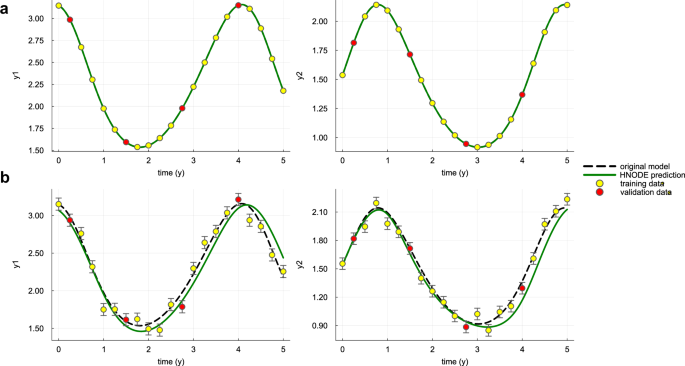
The dynamics predicted by the HNODE model trained on DS0.00 and DS0.05 (shown in panels a and b respectively) are compared with the original model. The points represent the observations of the system, divided into training and validation sets.
To assess the identifiability of α, we analyze its projection onto the null subspace of Hχ (Fig. 3). In both HNODE models, the norm of the projection exceeds δ, indicating the non-identifiability of the mechanistic parameter. These projections consist of both α and neural network parameters, suggesting a compensation between the neural network and the mechanistic parameter. This aligns with our expectations, as the first equation of Eq. (13) consists of a sum between a neural network and a mechanistic term involving α. It is thus plausible that the neural network, with its approximation properties, could adapt to changes in the mechanistic parameter α.
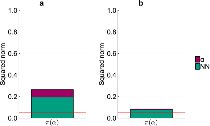
Squared norm of the projections of the parameter α onto the null subspace of Hχ for the models trained on DS0.00 and DS0.05 (panels a and b respectively). The total height of the bar corresponds to the squared norm of the projection, while the different components of the projection are depicted in different colors. The red line indicates the threshold to determine the identifiability of the parameter (0.05). Parameters with a squared norm of the projection exceeding this threshold are classified as locally non-identifiable.
In this simple scenario, we aim to demonstrate qualitatively that the projection of the mechanistic parameter onto the null subspace of Hχ effectively embodies a compensation between the mechanistic parameter and the neural network. To achieve this, we analyze the model behavior when the parameters of the trained HNODE model are perturbed along the direction identified by the projection (Fig. 4). The analysis reveals that, despite the sensitivity of the model dynamics to changes solely in the parameter α, moving along the projection allows a significant alteration of the value of α without impacting the overall model dynamics.
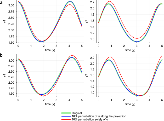
The dynamics predicted by the HNODE models trained on DS0.00 and DS0.05 (panels a and b respectively) are compared with the dynamics obtained perturbing the α value by 10% along the projection onto the null subspace of Hχ, and with the dynamics obtained perturbing solely α by 10%.
Such compensation hinders the identifiability of α, and our workflow terminates at this point. We conclude by showing that, in this scenario, the regularization of the cost function proposed by Yin et al.28 does not ensure an accurate estimation of α. Their proposed regularization involves minimizing the contribution of the neural network in the HNODE model. Mathematically, this approach consists of adding the following regularizer to the cost function:
where X is a grid of time points on the integration interval. To demonstrate that in this case this approach would not be effective, we sampled 50 values for α within the interval [0.013, 3] and trained the HNODE model keeping α fixed. This resulted in obtaining a neural network parameterization ({{boldsymbol{theta }}}_{alpha }^{NN}) for each α, yielding a profile for the regularizer:
For α ≤ 2, the value of α is not correlated with the ability of the HNODE model to fit the data (Supplementary Fig. 1), suggesting that the compensation holds in this region. If the inclusion of the regularizer enables the accurate estimation of α, the ground truth value (overline{alpha }) should correspond to the minimum of the regularizer profile R. However, our analysis indicates that this is not the case (Fig. 5). Therefore, in this scenario, using the regularizer would result in a biased estimation of the parameter.
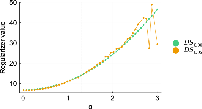
The profiles of R(α) for the models trained on DS0.00 and DS0.05 are plotted in the interval [0, 3]. The vertical dashed line denotes the ground truth value of α.
Cell apoptosis test case
The second test case is based on a model for cell death in apoptosis29, which constitutes a core sub-network within the signal transduction cascade that regulates programmed cell death. This model is known for the structural and practical non-identifiability of part of its parameters6. The equations defining the model are as follows:
In this context, we assume a lack of mechanistic knowledge about the entire equation related to y4. We selected this variable to maximize the challenge, as the corresponding equation contains the highest number of non-linear terms in the system. Our objective is to estimate all the parameters of the model. We assume knowledge of the variables directly influencing the dynamics of y4; thus, we model the unknown derivative of y4 with the neural network:
As in Lotka-Volterra, we assume a search space for the mechanistic parameters ranging from 10−2 to 102 times the ground truth value for each parameter. These ground truth values, derived from the values used by Aldridge et al.29, are specified in Supplementary Note 6, together with an analysis of the stiffness of the ODE system.
In the first scenario, we assume that all the system variables are observable. The observations are generated by numerically integrating Eq. (14) from 0 to 16 hours, with the parameters and initial conditions outlined in Supplementary Note 6. The trajectory is sampled every 0.8 hours, resulting in 21 observed time points. Similar to the previous test case, we consider a dataset DS0.00 without noise, and a dataset DS0.05 in which each time series is perturbed with zero-mean Gaussian noise with a standard deviation equal to 5% of its min-max variation. In this test case, after observing the integration in the first trials of the hyperparameter tuning, we manually switched to stiff configurations. These configurations include utilizing the TRBDF251 implicit Runge-Kutta ODE solver and the QuadratureAdjoint35 method for adjoint sensitivity computation. Additionally, the neural network architecture search spaces are expanded to include a deeper neural network (up to 6 hidden layers), with gelu as the activation function. The hyperparameters selected by the pipeline are reported in Supplementary Table 8, and the dynamics for y4, y5, y6, and y7 predicted by the trained HNODE models are presented in Fig. 6 (Supplementary Figs. 3 and 4 for the dynamics of all the variables). The trained HNODE model effectively fits the data.
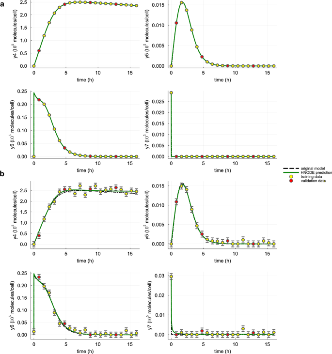
The dynamics of y4, y5, y6, and y7 predicted by the HNODE model trained on DS0.00 and DS0.05 (shown in panels a and b respectively) are compared with the original model. The points represent the observations of the system, divided into training and validation sets.
With the trained HNODE models, we proceed to the identifiability analysis and the CI estimations of the mechanistic parameters of the model (Table 2). Two of the model parameters, kd2 and kd4, are classified as identifiable, and this is empirically confirmed by the accuracy of their estimates (maximum relative error of 0.38% when estimated on the dataset without noise and 5.08% on the dataset with noise).
To understand why the other mechanistic parameters are classified as not identifiable, we analyze the components of the projections on the null subspace of Hχ. The analysis reveals the absence of neural network parameter components in both the HNODE models (Fig. 7 for the model trained on DS0.00, Supplementary Fig. 2 for analogous results obtained with the model trained on DS0.05). This implies that the parameter non-identifiability is not caused by compensations due to the neural network. Notably, the projections of parameters k1 and kd1 show almost equal contributions from both the parameters, and the same holds for the parameters k3 and kd3. This suggests the existence of local compensations between k1 and kd1, as well as between k3 and kd3.
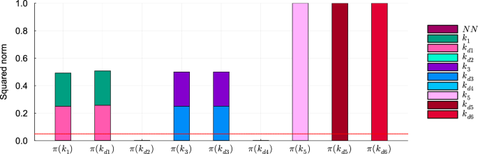
Squared norm of the projections of the mechanistic parameters onto the null subspace of Hχ for the model trained on DS0.00. The total height of the bar corresponds to the squared norm of the projection, while the different components of the projection are depicted in different colors. The red line indicates the threshold to determine the identifiability of the parameter (0.05). Parameters with a squared norm of the projection exceeding this threshold are classified as locally non-identifiable.
To assess the existence of such compensations and to evaluate the performance of our approach with a larger number of identifiable parameters, we fix kd1 and k3 to their ground truth values (36.0 h−1 and 24.48 cell ⋅ h−1 ⋅ 10−5 ⋅ molecules−1 respectively29) and execute the pipeline. The selected hyperparameters are listed in Supplementary Table 9; the dynamics predicted by the HNODE models effectively fit the experimental data (Supplementary Figs. 6 and 7). The results show that in this condition the identifiability of kd1 and kd3 is restored, allowing for the estimation of four model parameters with low relative error (Table 3).
To mimic more realistic conditions in the second scenario, keeping kd1 and k3 fixed to their ground truth values, we suppose that only the variables y5 and y6 are observable. We selected these variables because, within the mechanistic model, they represent the minimal subset that maximizes the number of identifiable parameters (Supplementary Note 16). The in silico observations are generated as in the first scenario. However, since only 2 out of 8 model variables are observable, trajectories are sampled every 0.4 hour to maintain a comparable amount of information in the training set, resulting in 42 time points. The hyperparameters tuned in the pipeline are listed in Supplementary Table 10, and the dynamics of the observable variables predicted by the HNODE models are shown in Supplementary Figs. 9 and 10.
In this scenario kd2, kd3, and kd4 are still identifiable (Table 4), and can be accurately estimated (maximum relative error of 0.17% when estimated on the dataset without noise, 11.64% on the dataset with noise), whereas k1 is not. The analysis of the components of the projections of the mechanistic parameters onto the null space of Hχ suggests that the non-identifiability of k1 in this scenario is caused by a compensation between k1 and the neural network (Fig. 8 and Supplementary Fig. 8).
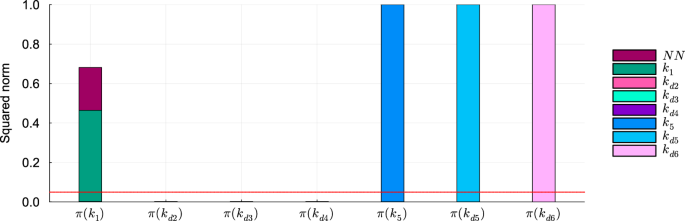
Squared norm of the projections of the mechanistic parameters onto the null subspace of Hχ for the model trained on DS0.00. The total height of the bar corresponds to the squared norm of the projection, while the different components of the projection are depicted in different colors. The red line indicates the threshold to determine the identifiability of the parameter (0.05). Parameters with a squared norm of the projection exceeding this threshold are classified as locally non-identifiable.
Yeast glycolysis model
The last test case is based on a model of oscillations in yeast glycolysis30, which has been frequently employed as a benchmark for inference in computational systems biology6,52. The model is described by the following system of ODE:
In this test case, we assume a complete absence of mechanistic knowledge concerning y1. This variable has been chosen to maximize the challenge, as its nonlinear oscillatory dynamics have proven to be particularly difficult for automatic identification of dynamical systems53. Our objective is to estimate all the parameters of the systems (except J0, which appears only in the derivative of y1, and therefore is not present in the HNODE model). As in the cell apoptosis case, we assume a knowledge of the variables directly influencing the dynamics of y1, thus the equation of y1 will be approximated by a neural network depending solely on y1 and y6. Given the greater number of system parameters compared to the first two test cases, we assume a search space ranging from 10−1 to 101 times the ground truth value for each mechanistic parameter. These ground truth values, derived from the values employed by Ruoff et al.30, are specified in Section Supplementary Note 18.
In the first scenario, we assume that all system variables are observable. The observations are generated by numerically integrating Eq. (15) from 0 to 6 min, using the parameters and initial conditions specified in Supplementary Note 18. The trajectory is sampled every 0.8 min (21 observation time points). We consider observation datasets with and without noise, labeled as DS0.00 and DS0.05 respectively. The noise dataset (DS0.05) is generated as in the two previous test cases. We execute the pipeline, switching to stiff configurations (as described for the cell apoptosis case) after observing the first trials of the initial step. The tuned hyperparameters are listed in Supplementary Table 17. The trained HNODE models fit the observations (Fig. 9 for the dynamics of the variables y1 and y2, Supplementary Figs. 11 and 12 for all the model variables).
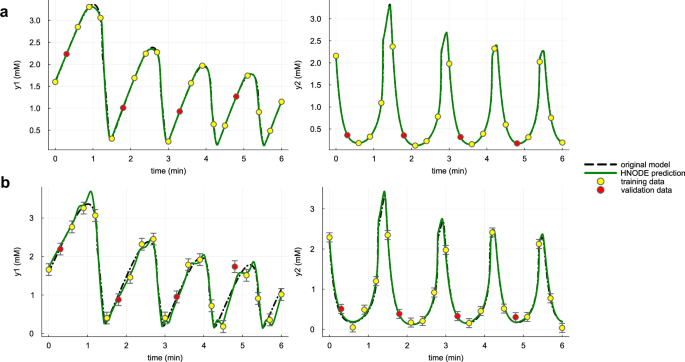
The dynamics of y1 and y2 predicted by the HNODE model trained on DS0.00 and DS0.05 (shown in panels a and b respectively) are compared with the original model. The points represent the observations of the system, divided into training and validation sets.
In the noiseless case, the pipeline assesses the identifiability of all the parameters, whereas, in the presence of noise, k1 is classified as not identifiable. By comparing the norm of the projections of the mechanistic parameters onto the null space of Hχ (Supplementary Fig. 13), we can notice that also when estimated on DS0.00, the norm of the k1 projection falls just below our identifiability threshold. In both cases, the projections of k1 are composed by k1 itself and by the neural network parameters, thus embodying a potential compensation between k1 and the neural network. This is plausible since the parameter k1 in the HNODE model directly multiplies the variable y1 parameterized by the neural network.
The identifiable parameters are estimated with a maximum relative error of 1.94% (Table 5) on DS0.00, with the ground truth value of the parameter always falling within the estimated CIs. When estimated on DS0.05, the maximum relative error of the identifiable parameter estimates is 52.60%, with the CIs containing the relative ground truth value for 11 out of 12 parameters. Given the challenge of discerning whether the relative error of parameter estimates originates from the lack of mechanistic knowledge or from the noise in the observation dataset, we attempted to estimate all parameter values using the fully mechanistic model on dataset DS0.05. The outcomes indicate that the mean and maximum relative errors obtained with our pipeline are consistent with what is obtained with the fully mechanistic model (Supplementary Note 24).
In the second scenario, we assume that only the variables y5 and y6 are observable. We chose these variables because, in the original model, all parameters are identifiable when y5 and y6 are observed6. Following a consistent approach with the previous test case, the in silico observations are generated as in the first scenario, with the sampling frequency halved to 0.4 minutes, resulting in 42 observed time points. The pipeline is run analogously to the first scenario. The tuned hyperparameters are listed in Supplementary Table 18, and the dynamics predicted by the HNODE model (Supplementary Figs. 14 and 15) fit the experimental data.
Similar to the first scenario, the results regarding parameter identifiability vary when the parameters are estimated on DS0.00 and DS0.05 (Table 6). When the parameters are estimated using the dataset without noise, the pipeline classifies six parameters as identifiable. However, when estimated using DS0.05, the parameters K1 and k4, classified as identifiable on DS0.00, are classified as non-identifiable. By analyzing the projections of the parameters onto the null subspace of Hχ (Fig. 10), we can notice that K1 is classified as non-identifiable on DS0.05, but its projection falls just above the threshold. Conversely, parameter k4 is classified as identifiable on DS0.00, yet its projection falls just below the threshold. Interestingly, on both datasets, the neural network parameters significantly contribute to the projection of nearly all non-identifiable mechanistic parameters, except for k2 and N. This observation is consistent with our findings on the cell apoptosis test case: when the unknown variable y1 is not observable, the neural network can compensate for changes in mechanistic parameters, also not directly linked to y1 in the HNODE model.
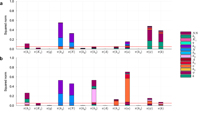
Squared norm of the projections of the mechanistic parameters onto the null subspace of Hχ for the model trained on DS0.00 and DS0.05 (panels a and b respectively). The total height of the bar corresponds to the squared norm of the projection, while the different components of the projection are depicted in different colors. The red line indicates the threshold to determine the identifiability of the parameter (0.05). Parameters with a squared norm of the projection exceeding this threshold are classified as locally non-identifiable.
The identifiable parameters are estimated with a maximum relative error of 9.26% on DS0.00. On the dataset with error DS0.05 the identifiable parameters are estimated with a maximum relative error of 11.05%. In both cases, the ground truth value consistently falls within the confidence interval estimated.
Discussion
We have introduced a pipeline for estimating mechanistic parameters and discussing their local identifiability within an incompletely specified mechanistic model. This workflow leverages the HNODE framework to embed the original model into a larger model, in which the unknown portions of the system are described by neural networks. The primary novelties of our work lie in our approach to conducting a global exploration of the mechanistic parameter search space and our method to evaluate the parameter identifiability. First, we include the initial values of mechanistic parameters into the hyperparameters to be tuned. This involves combining Bayesian Optimization with gradient-based search, with the goal of globally exploring the parameter search space. Second, to assess the local identifiability at-a-point of the parameters, we extend a classical approach for identifiability analysis in mechanistic models. Notably, identifiability analysis for HNODE models has not been previously investigated in the literature, which has predominantly focused on ensuring the identifiability of the mechanistic component through regularization of the training cost function26,28.
The primary limitations of our work include: (1) the assumption of having access to initial conditions for all state variables within systems, even under partial observability; (2) the computational cost associated with the hyperparameter tuning phase; (3) the intrinsic local nature of identifiability analysis; (4) the arbitrary selection of hyperparameters, ϵ and δ, for identifiability analysis; and (5) the methodology employed for estimating confidence intervals. All these limitations are discussed in the following paragraphs.
We assume knowledge of the initial states of all system variables, possibly with noise, even when only a subset of them is observable. In real-world scenarios, this assumption may not always be valid. While in certain cases, scientists have concrete physical insights into the system initial state, in others, initial concentrations need to be estimated alongside the parameters. Notably, this limitation is shared by other approaches to system identification6.
The initial phase of hyperparameter tuning and exploration of the mechanistic search space is the most computationally expensive step within the pipeline (for a discussion of the computational times required to run the pipeline across the different test cases, see Supplementary Note 26). We employed the TPE algorithm, and this algorithm has proven effective even in high-dimensional parameter search spaces, as evidenced by the Yeast Glycolysis test case, featuring 13 mechanistic parameters and 6 hyperparameters. However, employing the TPE algorithm entails sequentially repeating the training of the candidate HNODE model, each time with a limited number of epochs. It is important to note that the problem of hyperparameter tuning is a long-standing problem and different approaches have been proposed for this goal54. These approaches range from random and grid search to Bayesian optimization and genetic algorithms: in this work, we did not conduct a comparative analysis of TPE performance against other hyperparameter tuning methods.
The local nature of our identifiability analysis implies that it might overlook parameter non-identifiability if distinct parameterizations leading to similar model simulations are isolated in the search space, as separate local minima of the cost function.
The hyperparameters ϵ and δ used for identifiability analysis, although related, have different meanings. The threshold ϵ intuitively distinguishes what we assume to be negligible changes in the HNODE model behavior from non-negligible changes. This hyperparameter is also present in existing Hessian-based methods for identifiability analysis of mechanistic models42. The threshold δ, introduced in our method, intuitively quantifies how much it is possible to perturb the mechanistic parameter with a negligible effect on the model simulations. δ has been introduced to overcome the limitation of the dominant parameter approach in the context of HNODE. Existing Hessian-based methods for identifiability analysis of mechanistic models42 primarily categorize parameters as non-identifiable if they have the highest projection (in absolute value) onto eigenvectors associated with null eigenvalues. We decided against using this approach because we observed empirically that in HNODE models when compensation occurs between the neural network and mechanistic parameters, the dominant parameter in the null direction is typically a neural network parameter. Thus, considering only the dominant parameter, we risk overlooking the role of the mechanistic parameter. In our test cases, we employed ϵ = 10−5 and δ = 0.05. The results of the first two test cases are quite robust to the choice of ϵ and δ (Supplementary Notes 4 and 17). However, the third test case is more complex: here changes in ϵ and δ would lead to different results for certain parameters (Supplementary Note 25).
The fifth limitation of our work is the CI estimation. The FIM-based approach we employed has several limitations55. By using it, we implicitly assume the unbiasedness and normality of our estimators47. Additionally, since our estimators are not linear, the CIs estimated are only lower bounds of the real CIs47. We opted for this method because of its computational advantages over other methods, such as likelihood profiling or bootstrapping-based methods13,55, which would necessitate multiple trainings of the HNODE model.
We tested our pipeline in various in silico scenarios of increasing complexity, assuming a partial lack of mechanistic knowledge in three models acknowledged as benchmarks in computational biology. In each test case, we replace either a portion or an entire equation of the system with a neural network, creating a hybrid model in which the neural network influences the dynamics of all system variables (as detailed in Supplementary Note 27). These tests encompass various conditions, including different levels of noise in the training data and different assumptions regarding the observability of the system variables. Across all the examined scenarios, our pipeline consistently enabled the analysis of parameter identifiability and the accurate estimation of identifiable parameters.
Despite its limitations, the proposed workflow represents an initial step toward adapting traditional methods utilized in entirely mechanistic models to the HNODE modeling scenario. In future works, we aim to address the limitations of the pipeline. Firstly, we will consider different state-of-the-art approaches for hyperparameter tuning, such as Gaussian process56, evolutionary54, and genetic approaches57, comparing their performances with TPE. Secondly, we plan to expand the number of test cases to derive a less arbitrary choice of the thresholds ϵ and δ, which could vary based on the number of parameters in the HNODE model. Thirdly, we intend to compare the FIM-based method for estimating CIs with other approaches that have demonstrated greater reliability in completely mechanistic models, as described by Kreutz et al.13 and Joshi et al.55.
Methods
Algorithmic setup
All the results presented for the test cases described in the Results Section have been obtained employing the following hyperparameters. The observation data point datasets are partitioned into training and validation sets with an 8:2 ratio. The first stage of the hyperparameter tuning consists in 500 iterations of TPE: in each trial, the HNODE model is trained for 500 epochs using Adam optimizer. In the second stage of the hyperparameter tuning (performed only on datasets with noise) the model is trained for 2000 epochs in each trial. The comprehensive training of the HNODE model encompasses 10000 epochs utilizing the Adam optimizer. Subsequent refinement involves the application of the L-BFGS algorithm until convergence, with a maximum of 5000 epochs (performed only on noiseless datasets). The optimized mechanistic parameters are clipped to the lower or upper bounds of the parameter search spaces when they exceed those limits. Each model is trained with 10 initializations of the neural network, with weights initialized using Glorot Uniform58. The training resulting in the lowest validation cost is then selected. The identifiability analysis is performed using the thresholds ϵ = 10−5 and δ = 0.05; a discussion regarding these thresholds is provided in the Discussion Section.
Implementation
All the computations have been run on a Debian-based Linux cluster node, with two 24-core Xeon(R) CPU X5650 CPUs and 250 GB of RAM. The code is implemented in Julia v1.9.159, using the SCiML environment23, a software suite for modeling and simulation that also incorporates machine learning algorithms. The hyperparameter tuning has been performed with Optuna60.


Responses