Random memristor-based dynamic graph CNN for efficient point cloud learning at the edge
Introduction
With the widespread adoption of 3D sensors in everyday devices, such as mixed reality headsets, automobiles, drones, and even smartphone cameras, there has been an explosive growth in the volume of 3D data. Point clouds1 have emerged as a mainstream method for representing the shape and geometry of 3D objects through a series of discrete points (Fig. 1a). The easy accessibility of point cloud data has significantly expanded its applications across a wide range of fields such as augmented and virtual reality (AR/VR), autonomous driving, robotics, and photography. Often operating at the edge, where computing resources and battery life are limited, these application scenarios underscore the importance of accurately, promptly, and efficiently learning of point cloud data.
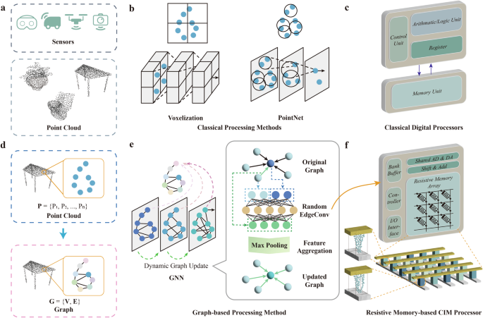
a Point cloud data, represented by a series of discrete points, is widely applied in everyday life with the popularization of 3D sensors in devices like mixed reality headset, automobiles, drones, and smartphone cameras. b Traditional machine learning approaches for handling point clouds: Left: Method of voxelizing point clouds and using 3D convolutional operations for processing; Right: Method of representing point clouds as point sets and directly processing them through neural networks. c The traditional von Neumann architecture of processors, with separate computation and storage units, introduces significant data transfer overhead. d We convert the point cloud into a graph representation, where each point serves as a vertex in the graph, and the edges are determined by the features of the points. e Our random dynamic graph CNN method. Left: The network dynamically updates the vertex features and connections, extracting hierarchical information. Right: The random EdgeConv operation. The central vertex features and neighboring vertex features are concatenated and passed through a random CNN to obtain edge features. The updated central node features are calculated by aggregating the edge features associated with edges emanating from all neighbouring vertices, and new graph connections are computed based on the updated features. f Our memristor-based Computing-In-Memory (CIM) system. Leveraging the in-memory computing capability of memristor, it reduces data transfer overhead and utilizes the intrinsic stochasticity to obtain a random conductance matrix for the physical implementation of random CNN weights.
However, conventional software-hardware pairs face significant challenges. In terms of software, so far there are multiple methods to learn 3D points (Fig. 1b). The first method involves voxelizing the point cloud data. Voxelization converts the point cloud into a regular grid of 3D voxels, transforming the irregular point cloud into a structured format that can be processed using 3D convolutional operations2,3. However, voxelization can result in high memory consumption and computational cost, especially with fine-grained voxel grids. The second is to directly process point cloud data4,5 by grouping and sampling within the point cloud to form a point set representation, which allows for the extraction of point cloud features without converting them into a different representation. While these approaches avoid the information loss associated with voxelization, they can still be expensive in training and struggle with capturing fine-grained geometric relationships between points.
In terms of hardware, conventional processors struggle to deliver the energy efficiency required for edge processing point cloud data (Fig. 1c). Traditional von Neumann architectures feature physically separated processing and memory units. This separation leads to substantial data transfer overheads, known as the von Neumann bottleneck6. Moreover, due to the complexity of processing point cloud data, even high-performance GPUs struggle to meet the requirements for real-time processing7. This challenge is more pronounced in edge devices, where computational resources are significantly constrained.
To address the aforementioned challenges, we have co-designed software and hardware, random memristor-based dynamic graph CNN (RDGCNN).
Firstly, we transform point cloud data into graph data8,9, where points serve as vertices of the graph (Fig. 1d). The edges are computed and dynamically updated based on vertex features, facilitating the flow of information among neighboring nodes. This transformation into a graph naturally accommodates the irregular structure of point clouds, eliminating the need for voxelization and thereby avoiding information loss. Moreover, graph data adeptly captures the geometric structural features of the 3D point cloud.
On the software front, we have developed a random dynamic graph CNN to learn point clouds (Fig. 1e). Graph Neural Networks10 (GNNs) update graph node feature representations through information propagation among nodes, capturing both local structures and global topologies within point data. To reduce training cost, we devised a random EdgeConv9 to create a local neighborhood graph in feature space and perform convolutional operations on the connections between adjacent points. Unlike traditional GNNs, the edges in the point cloud graph dynamically update during embedding. Additionally, the weights of EdgeConv are fixed and random, avoiding the tedious training of conventional GNNs. Through iterative updates of vertex and edge embeddings via random EdgeConv, the feature representations obtained can serve various downstream tasks through a lightweight trainable task-dependent head.
At the hardware level, we leverage the in-memory computing capability of memristor and its intrinsic randomness to physically implement random EdgeConv layers (Fig. 1f). As a non-volatile memory device11,12,13,14,15,16,17,18,19, each memristor not only embodies the synaptic weight through analog conductance but also computes in-situ utilizing Ohm’s law and Kirchhoff’s current law for multiplication and accumulation (MAC)20,21,22,23,24,25,26,27. This approach significantly reduces the energy and time expenditures associated with traditional von Neumann architectures28,29,30,31,32,33,34,35,36. Furthermore, the uncertainty in ion migration during the electroforming process in memristor devices can cause variations in conductance values37,38,39. This intrinsic randomness often complicates the precise mapping of weights, deemed a disadvantage. However, we turn this into an advantage by utilizing the intrinsic randomness to realize truly random, large-scale and low-cost hardware random weights.
We implemented our co-design on a 40 nm memristor macro and validated the effectiveness of our approach on three canonical point cloud tasks: classification, part segmentation, and semantic segmentation. On the ModelNet4040, we achieved classification accuracy of 89.75%. On ShapeNet41, and S3DIS42 datasets, we achieved mean Intersection over Union43 (mIoU) of 83.67%, and 46.35%, respectively. Furthermore, the energy consumption of our system is reduced by 54.2%, 39.5%, and 35.3% compared to state-of-the-art (SOTA) GPUs. Moreover, the training complexity is reduced by 96.4%, 53.5%, and 68.1% compared to fully trainable baseline. Our co-design paves the way for future efficient and rapid point cloud applications at the edge.
Results
Software-hardware co-design of RDGCNN
Our RDGCNN algorithm, as shown in Fig. 1d, e, first constructs a graph G = (V, E) for the input point cloud data. Each point in the point cloud becomes a center vertex in the sub-graph, and edges are created to connect each point with its n nearest neighboring points determined by the relationships of the neighbouring points. We use the K-Nearest Neighbors (KNN) algorithm to construct the local graph structure. For each pair of adjacent points, the edge features are defined by a non-linear function hθ (xi, xj − xi), where xi represents the feature of the center point for capturing global information, and xj − xi represents the feature difference of the neighbor for extracting local geometric information. The function hθ is parameterized by a CNN with random weights, implemented by random analog memristors, to obtain the edge features eij. After extracting features for the n nearest neighbors of the center point xi, the edge features are aggregated using a permutation-invariant max pooling function to obtain the updated center point feature xi′. After completing the feature update process, the new graph G′ = (V′, E′) is obtained by recalculating the n-nearest neighbors based on the updated node features. This dynamic construction of G(l) = (V(l), E(l)) is iteratively performed at each layer l, gradually extracting higher-level features and gathering points in semantic space. For downstream tasks, the hierarchical features are concatenated and passed to lightweight trainable task-dependent heads in digital domain, enabling applications such as classification and segmentation.
Inspired by matrix decomposition methods such as Singular Value Decomposition44 (SVD) and low-rank decomposition45, we split a random EdgeConv layer with a k ×k ×c filter size and d filters into two random sub-layers (Fig. 2a). The first layer has d′ filters with a k × k × c filter size, while the second layer has d filters with a 1 × 1 × d′ filter size (d′ is much smaller than d). The first layer compress n×c features to a low-rank intermediate feature subspace of dimension n×d′. The second layer then approximates the original output features of dimension n×d. This splitting approach reduces the parameter size to (frac{{d}^primetimes{k}times{k}times{c}+{d}^primetimes{d}}{{d}times{k}times{k}times{c}}), and the computational complexity changes from O(dk2c) to O(d′k2c) + O(dd′). By adjusting the subspace dimension d′, a tradeoff between parameter size and performance can be achieved.
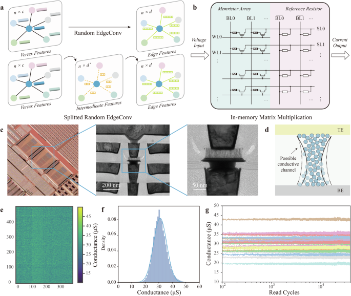
a Schematic of random EdgeConv splitting to reduce parameter count. We split one EdgeConv layer into two sub-layers. b Hardware implementation of in-memory matrix multiplication on memristor macro. Inputs are converted to voltages and fed into bit-lines, carrying vector-matrix multiplication via Ohm’s and Kirchhoff’s laws. Output currents from source lines are accumulated from memristor array and reference resistor output. c Optical photos of the memristor array and cross-sectional Transmission Electron Micrograph (TEM) of a single 1-transistor-1-memristor cell (scale bar: 200 nm and 50 nm). d Physical origin of intrinsic stochasticity in memristor. e Conductance map of memristor sub-array. f Histogram of the conductance. g Retention of memristors.
Figure 2b schematically illustrates the in-memory matrix multiplication realized on a memristor macro. The random weights are realized with the intrinsic stochasticiy provided by memristor array, where each memristor cell is subtracted from a fixed reference resistor (with a conductance of 30 µS) to obtain positive and negative weights. The inputs are converted to voltages through digital-analogue convertors (DACs) and then fed into the bit-lines. The vector-matrix multiplication is achieved based on Ohm’s law and Kirchhoff’s law. The output currents from the memristors and the reference resistors are accumulated and digitized (see Supplementary Fig. 1 for memristor based hybrid analog-digital computing platform).
Figure 2c shows the chip photograph and transmission electron microscope (TEM) cross-sectional imaging of the memristor array, as well as nanoscale TaN/TaOx/Ta/TiN memristor devices integrated with complementary metal-oxide-semiconductor (CMOS) at the back-end-of-line process, fabricated in a test chip using the 40 nm technology node (see Supplementary Fig. 2 for memristor device characterization). The conductance of the memristor is controlled by the formation of conductive channels based on oxygen vacancies in the TaOx layer. Under the same electrical breakdown conditions, oxygen vacancies are generated in TaOx, which then migrate to form conductive channels and eventually transition to a high-conductance state. The heterogeneity in the position, shape, and vacancy concentration of the conductive channels across different devices leads to a random conductance (i.e., write noise) distribution within the memristor array (Fig. 2d). Figure 2e shows the conductance map of a 360 × 488 memristor sub-array. The resistance distribution follows a Gaussian distribution with a mean value around 30.9 µS and standard deviation around 4.9 µS (Fig. 2f). Figure 2g demonstrates the retention of the memristor devices over 40,000 reading cycles, where the device conductance fluctuations (i.e., read noise) are relatively small compared to write noise.
3D point cloud classification
First, we validated the effectiveness of our co-design on point cloud classification tasks with ModelNet4040 dataset. ModelNet40 is a widely used dataset for point cloud classification, consisting of 12,311 models from 40 different categories. Each model contains 1024 points, with each point having coordinate information (x, y, z). The system is expected to assign the entire point cloud to a specific category, such as recognizing it as a table, chair, laptop, motorbike, etc. Each point cloud model is first transformed into a graph with a selected number of nearest neighbors (n = 20). The model architecture is shown in Fig. 3a, where the graph first goes through 4 splitted random EdgeConv layers to extract features. Then, the hierarchical features are concatenated together through residual connections and further aggregated through a fusion layer. Finally, a lightweight trainable classification head is used for predicting the class (see Supplementary Fig. 3 for detailed network structure). During the model training process, the splitted random EdgeConv layers’ weights stay fixed. Only the weights of the classification head need to be updated, resulting in substantially reduced computational complexity compared to the baseline dynamic graph CNN (DGCNN)9 model with fully trainable EdgeConv layers.
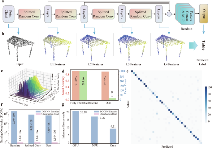
a Schematic of RDGCNN for point cloud classification task on ModelNet40 dataset. b Experimental input and feature evolution of a chair model from the ModelNet40 dataset. c Weight distributions of different random EdgeConv layers. d Testset classification results and parameter count comparisons of trainable software DGCNN baseline and our co-design. e Confusion matrix of the classification results of our co-design on ModelNet40, with dominating diagonal elements. f Comparison of training complexity between the fully trainable DGCNN, DGCNN with splitted EdgeConv, and RDGCNN with splitted random EdgeConv (ours). g Comparison of inference energy between GPU, NPU, and our co-design.
Figure 3b illustrates the experimental input and feature evolution of the point cloud graph after random EdgeConv layers, as revealed by the color variations of different nodes in a sample selected from the chair category of ModelNet40. The color variations are calculated based on the distance to a specific node in the feature space. The node features are accumulated from dynamically generated graph neighboring edges, gradually extracting higher-level information such as topological structure. Finally, the classification head predicted the class label. Figure 3c illustrates the random EdgeConv weights following Gaussian distributions in different layers. The first layer does not undergo splitting, while the second to fourth layers employ splitted random EdgeConv. The testset classification results and parameter comparisons are shown in Fig. 3d. The baseline DGCNN model with fully trainable EdgeConv layers on the GPU achieves an accuracy of 91.45%. Meanwhile, our co-design achieves a classification accuracy of 89.75%, with only 1.7% decrease. In terms of trainable parameter count, our co-design exhibits a reduction of 92.5% compared to the trainable model (see Supplementary Fig. 6a for detailed parameter count comparison), making it highly favorable for edge hardware deployments with limited computing resources. Figure 3e presents the confusion matrix of the prediction results of our co-design on ModelNet40, showing dominant diagonal elements for most categories.
In addition to demonstrating its classification performance, we also analyzed the training costs and energy efficiency. We compared the fully trainable software baseline with trainable splitted EdgeConv and splitted random EdgeConv in terms of training costs (as shown in Fig. 3f). Compared to the software baseline, splitted EdgeConv and splitted random EdgeConv reduced the training workload by 56.6% and 96.4%, respectively. We also compared the inference energy reduction of our co-design relative to the GPU (Nvidia A100) and NPU (Nvidia Jetson Nano). As is shown in Fig. 3g, compared to the GPU and NPU, our co-design reduces the inference energy consumption by 54.2% and 37.3%, respectively, requiring only 9.51 mJ per sample (see Supplementary Table. 1 for detailed energy breakdown).
3D point cloud part segmentation
We extended our co-design approach to the part segmentation task on the ShapeNet41 part dataset. Compared to classification, part segmentation is a more fine-grained task that involves segmenting different parts of objects, commonly used in fields such as robot grasping and object modeling. For example, given a model of an airplane, the system is expected to identify key components such as the fuselage, wings, tail, and engines. The ShapeNet dataset consists of 16,881 3D shapes from 16 object categories, annotated with a total of 50 parts. As is shown in Fig. 4a, the point cloud data is first processed by a spatial transformation network, followed by three splitted random EdgeConv modules for feature extraction. The hierarchical features are concatenated through residual connections and passed through a fusion layer for aggregation. Subsequently, they are fed into a lightweight segmentation head for point-wise classifications (see Supplementary Fig. 4 for detailed network structure). Figure 4b presents the experimental results showing the feature evolution of points in an airplane model from the ShapeNet dataset. The color of each point represents the distance to the red point in the feature space. It can be observed that in deeper layer feature space, even if there is a significant distance between them in the original input space, semantically similar structures can be captured. For example, the wings gradually converge to the same color in the figure. We measure the performance of segmentation through mIoU and compare it with the trainable software baseline. Our co-design achieved a mIoU of 83.67%, with only an 1.90% decrease (Fig. 4c). In most categories, our co-design can achieve performance similar to that of the software. In specific categories such as motorbike, due to the imbalance in sample numbers between categories and the analogue computing noise, our co-design shows a more noticeable decline compared to the software baseline (see Supplementary Fig. 7a for accuracy metrics). Compared to the baseline, our co-design has a 89.8% reduction in the number of parameters (Fig. 4d, see Supplementary Fig. 6b for detailed parameter count comparison). Figure 4e visualizes randomly selected part segmentation results using our co-design on ShapeNet. Different colors represent different parts.
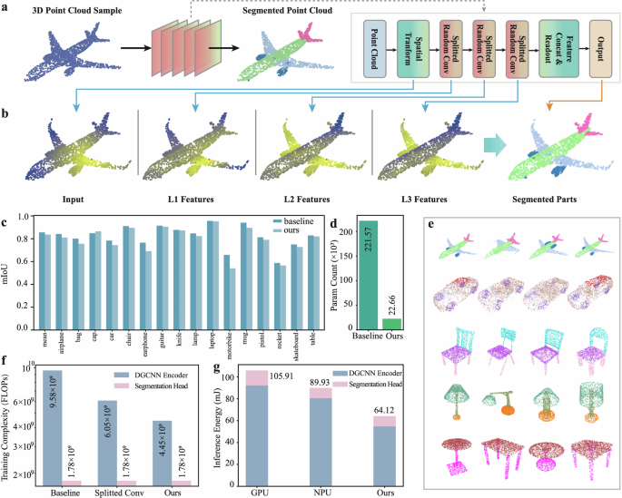
a Schematic of RDGCNN for the part segmentation task on the ShapeNet dataset. b Experimental feature evolution of points in an airplane model from the ShapeNet dataset. c Comparison of part segmentation results of software trainable DGCNN baseline and our co-design. d Parameter count comparisons of trainable software DGCNN baseline and our co-design. e Representative segmentation results of our co-design. f Comparison of training costs between the fully trainable DGCNN, DGCNN with splitted EdgeConv, and RDGCNN with splitted random EdgeConv (ours). g Comparison of inference energy between GPU, NPU, and our co-design.
We also analyzed the training cost and energy efficiency for the part segmentation task. We compared the fully trainable DGCNN software baseline with splitted trainable EdgeConv and RDGCNN in terms of training complexity (as shown in Fig. 4f). Compared to the fully trainable DGCNN, splitted EdgeConv and RDGCNN reduced the training cost by 36.8% and 53.5%, respectively. We also compared the inference energy reduction of our co-design relative to the GPU (Nvidia A100) and NPU (Nvidia Jetson Nano). As is shown in Fig. 4g, compared to the GPU and NPU, our co-design reduces the inference energy consumption by 39.5% and 28.7%, respectively, requiring only 64.12 mJ per sample (see Supplementary Table. 1 for detailed energy breakdown).
3D point cloud semantic segmentation
We further validated the effectiveness of our co-design on a more complex semantic segmentation task. Unlike part segmentation, which focuses on parts within a single object, semantic segmentation aims to understand the scene at a higher level by identifying and labeling entire objects. It is pivotal for applications that require scene understanding and contextual awareness, such as autonomous navigation and environmental mapping. We evaluated our co-design’s efficacy on the Stanford Large-Scale 3D Indoor Spaces Dataset (S3DIS)42 for the semantic segmentation task. This dataset consists of 3D scanned point clouds from six indoor areas, totaling 272 rooms. Each point belongs to one of thirteen semantic categories, such as floor, bookshelf, chair, ceiling, beam, and clutter. The network architecture used for this task is similar to the part segmentation model, with the difference being that the model’s output is a probability distribution for the semantic object category for each input point, rather than a category vector. As is shown in Fig. 5a, the point cloud data undergoes feature extraction through three splitted random EdgeConv modules, followed by aggregation of hierarchical features. The aggregated features then enter the lightweight trainable segmentation head to output the probability distribution of point categories (see Supplementary Fig. 5 for detailed network structure).
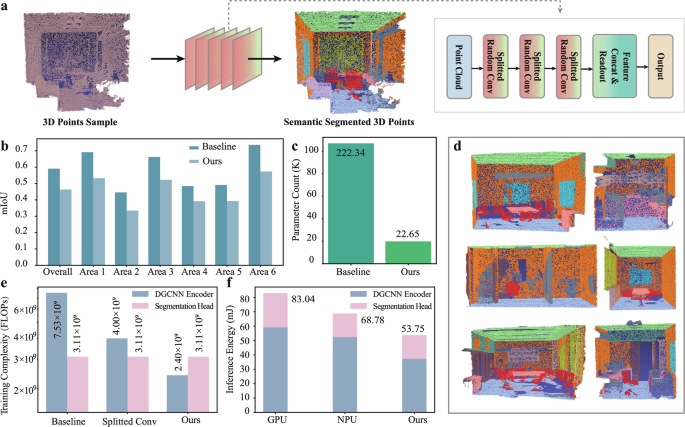
a Schematic of RDGCNN for the semantic segmentation task on S3DIS dataset. b Comparison of semantic segmentation results of each test area in a 6-fold cross-validation between software trainable baseline and our co-design. c, Parameter comparison of trainable software baseline and our co-design. d, Representative semantic segmentation results of our co-design. e, Comparison of training costs between the fully trainable DGCNN, DGCNN with splitted EdgeConv, and RDGCNN with splitted random EdgeConv (ours). f, Comparison of inference energy between GPU, NPU, and our co-design.
To evaluate the performance of our co-design, we use 6-fold cross-validation. As shown in Fig. 5b, compared to the trainable DGCNN baseline, our co-design achieved an overall mIoU of 46.35%, with a 12.73% decrease (see Supplementary Fig. 7b for accuracy metrics). In terms of the number of parameters, our co-design saw a reduction of 89.8% compared to the fully trainable baseline (Fig. 5c, see Supplementary Fig. 6c for detailed parameter count comparison). Figure 5d visualizes the semantic segmentation results of our co-design on S3DIS dataset, where different colors represent different semantic regions. We also analyzed the training overhead and energy efficiency on the semantic segmentation task. We compared the training costs of a fully trainable DGCNN, a DGCNN with trainable splitted EdgeConv, and our RDGCNN (as shown in Fig. 5e). Compared to the software baseline, DGCNN with trainable splitted EdgeConv and RDGCNN reduced the training complexity by 46.9% and 68.1% respectively. We also compared the inference energy reduction of our co-design relative to a GPU (Nvidia A100) and an NPU (Nvidia Jetson Nano). As is shown in Fig. 5f, compared to the GPU and NPU, our co-design reduced inference energy consumption by 35.3% and 21.9% respectively, requiring only 53.75 mJ per sample (see Supplementary Table. 1 for detailed energy breakdown).
Noise robustness analysis on conductance fluctuation
We further demonstrate the robustness of our co-design to read noise in memristors. Memristor primarily has two types of noise: write noise due to programming stochasticity and read noise due to fluctuation in charge transport. In our co-design, we utilize the former as a source for random weights to physically implement random EdgeConv. The latter, caused by thermal fluctuations or Random Telegraph Noise (RTN), leads to stochasticity in charge movement, resulting in slight changes in conductance over time (Fig. 6a). Figure 6b shows the conductance fluctuations of memristor after 10,000 reads. As the number of reads increases, the fluctuations slightly increase, but the overall fluctuation remains around 1.5% (the amplitude is determined by the standard deviation divided by the mean). We simulated various levels of read noise (Fig. 6c) from 1.5% to 9%, and modeled the impact of this noise on network performance across three tasks. Figure 6d, e, f respectively show the impact of different levels of noise on performance in point cloud classification, part segmentation, and semantic segmentation tasks. As the level of disturbance increases, the performance of the network gradually decreases. In the classification task, the model maintains a relatively good classification accuracy (over 80%) when the disturbance amplitude is within 4.5%. In the part segmentation task, the model is more robust to noise, still achieving an overall mIoU of about 80% even under a 6% fluctuation amplitude. For semantic segmentation, the model is more sensitive to read noise compared with classification and part segmentation, attaining in less than 20% mIoU when noise level exceeds 4.5% (see Supplementary Fig. 8 for more results with smaller noise fluctuation levels).
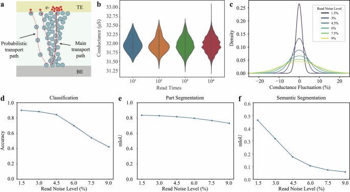
a Physical origin of conductance fluctuation in memristor. b Experimental read noise of memristor over 10,000 cycles. c, Illustration of simulated conductance fluctuation of different levels. d Classification accuracy on ModelNet40 under various conductance fluctuation levels. e Part segmentation performance on ShapeNet under various conductance fluctuation levels. f Semantic segmentation performance on S3DIS under various conductance fluctuation levels.
Discussion
In this research, we introduce a novel hardware-software co-designed system using RDGCNN and memristor for efficient and affordable learning of point cloud data, suited for edge applications like mixed reality, autonomous vehicles, and embodied AI. In this work, we implemented RDGCNN on a 40 nm fully integrated memristor array, which performed point cloud classification, part segmentation, and semantic segmentation tasks. Compared to state-of-the-art digital hardware, our co-design delivers energy consumption (training complexity) reduction of 54.2%, 39.5%, and 35.3% (96.4%, 53.5%, and 68.1%) on these three representative tasks, while achieving high classification accuracy and segmentation mIoU comparable to the software. Our co-design not only reduces the energy consumption substantially but also minimizes the training overhead, making it significantly more efficient and economical for real-time, high-performance edge applications. This innovative approach leverages the inherent randomness of memristor to enhance processing capabilities and paves the way for future edge computing in handling complex 3D datasets.
Method
Fabrication of random memristor chips
The memristor array was fabricated using 40 nm technology and features a 1T1R configuration. Each cell is located between the metal 4 and metal 5 layers in the backend-of-line process, with a structure comprising a bottom electrode (BE), a top electrode (TE), and a transition-metal oxide dielectric layer. The BE via was created using photolithography and etching techniques, filled with TaN through physical vapor deposition, and topped with a 10 nm TaN buffer layer. Subsequently, a 5 nm Ta layer was deposited and then oxidized to form an 8 nm TaOx dielectric layer. Finally, a 3 nm Ta layer and a 40 nm TiN layer were sequentially added via physical vapor deposition to construct the TE. The remaining interconnection metals were added using a standard logic process. BE connections were shared by cells in the same row, while TE connections were shared by cells in the same column, forming a 512 × 512 crossbar array. The 40 nm memristor chip exhibited high yield and strong endurance after being post-annealed at 400◦C for 30 minutes in a vacuum.
The hybrid analog-digital computing system
The hybrid analog-digital computing system includes a 40 nm memristor computing-in-memory chip and a Xilinx ZYNQ system-on-chip (SoC) mounted on a printed circuit board (PCB). This setup delivers parallel 64-way analog voltage inputs, produced by an 8-channel digital-to-analog converter (DAC80508, TEXAS INSTRUMENTS) with 16-bit resolution, covering a range from 0 V to 5 V. For signal collection, the convergence current is converted to voltages using trans-impedance amplifiers (OPA4322-Q1, TEXAS INSTRUMENTS) and read with a 14-bit resolution analog-to-digital converter (ADS8324, TEXAS INSTRUMENTS). The system integrates both analog and digital conversions onboard. During vector-matrix multiplications, a DC voltage is applied to the bit lines of the RRAM chip via a 4-channel analog multiplexer (CD4051B, TEXAS INSTRUMENTS) and controlled by an 8-bit shift register (SN74HC595, TEXAS INSTRUMENTS). The result current from the source line is converted to voltages and transferred to the Xilinx SoC for further processing.
Training details of classification on ModelNet40
The detailed network architecture used for the classification task is shown in Supplementary Fig. 3. In our model, we employ four random EdgeConv layers to capture geometric features, each supported by three splitted convolutional layers with dimensions of 32, 32, 64, and 128, with rank of 12. Following the computation in each EdgeConv layer, we update the graph using the new features to guide the next layer. For all EdgeConv layers, we set the nearest neighbor count, k, to 20. Multi-scale features are harvested through shortcut connections, and an additional splitted random 1D convolutional layer with a size of 1024 and rank of 12 is used to integrate these features into a 512-dimensional point cloud by merging outputs from earlier layers. Global features of the point cloud are extracted via global max/sum pooling and then transformed through two subsequent fully-connected layers sized 512 and 256. The last two layers include dropout at a 50% keep rate and feature LeakyReLU activation and batch normalization. We employ Stochastic Gradient Descent (SGD) with an initial learning rate of 0.1, gradually decreasing it to 0.001 through cosine annealing. The momentum setting for batch normalization is maintained at 0.9. Our batch size is set at 32, with the momentum at 0.9. We train the model for 250 epochs.
Training details of part segmentation on ShapeNet
The detailed network structure is depicted in Supplementary Fig. 4. Following a spatial transformer network, three EdgeConv modules are implemented. The first module include a splitted convolutional layer with dimension of 64 and rank of 12. The following two modules each consist of two splitted convolutional layers with dimension of 64 and rank of 12. Information from these layers is concatenated using a splitted random 1D convolutional layer withs dimension of 1024 and rank of 12. The neighbour count k is set to 40. Shortcut connections integrate outputs from all EdgeConv layers as local feature descriptors. Subsequently, the pointwise features are processed through three shared fully-connected layers with dimensions of 256, 256, and 128. Similar to our classification network, batch normalization, dropout, and ReLU are incorporated throughout this configuration. We adopt the same training setting as the classification task. We train the model for 200 epochs.
Training details of semantic segmentation on S3DIS
The network structure used for semantic segmentation is similar to classification model, as is shown in Supplementary Fig. 5. Three EdgeConv modules are used. The first module include a splitted convolutional layer with dimension of 64 and rank of 12. The following two modules each consist of two splitted convolutional layers with dimension of 64 and rank of 12. Information from these layers is concatenated using a splitted random 1D convolutional layer with dimension of 1024 and rank of 12. The neightbour count k is set to 20. Shortcut connections integrate outputs from all EdgeConv layers as local feature descriptors. Subsequently, the pointwise features are processed through a shared fully-connected layers with dimensions of 256. Similar to our part segmentation network, batch normalization, dropout, and ReLU are incorporated throughout this configuration. We adopt the same training setting as the classification task. We train the model for 100 epochs for each test area.


Responses