Spiking neural networks for nonlinear regression of complex transient signals on sustainable neuromorphic processors

The pioneering work of neuromorphic computing was described in¹ following another strategy of chip architecture as in the case of von-Neumann computer processors. Neuromorphic chips are regarded to be brain-inspired leading to a different signal processing as in the case of CPU/GPU chips. Due to their sparse nature, spiking neurons outperform forward and backward passes through a neuromorphic network with much less energy than von-Neumann chips. Moreover, spiking neural networks (SNN) are inherently recurrent and parallel² leading to the possibility of performing mathematical operations simultaneously and recursively. SNNs are known as neural networks of the third generation to be implemented on neuromorphic architecture resulting in low-power operations³ compared to traditional artificial neural networks (ANN) of the second generation. These ANNs of 2^nd generations have been successfully explored for a wide range of scientific purposes such as uncertainty quantification^4,5, fluid^6,7,8,9 and solid mechanics^10,11, biomechanics and mechanobiology¹² with applications in biomedicine^{13,14,15,16,17}. Targeting especially nonlinear regression tasks, ANNs can be developed successfully from the mathematical point of view for solving nonlinear differential equations with a physical application (e.g. material modeling)^{18,19,20,21,22,23,24,25,26,27}.

However, even though promising new possibilities for regression tasks are offered by neuromorphic architectures, they were mostly applied to classification problems and hardly to function approximation²⁸.

ANNs of the second generation have been successfully implemented in nonlinear regression but several computational bottlenecks arise as a result of their use, such as high memory access for model initialization, access latency, and throughput²⁹ leading to an increased demand for computational resources. These ANN attributes are due to the suboptimal nature of matrix multiplication depending on data communication and memory. However, human brains perform classification tasks such as image recognition and natural language processing^30,31 with significantly less energy^31,32 and incorporating discrete signals to communicate with each other. Neuromorphic chips being analog, digital, or mixed comprise small units mimicking the neurons in the brain such as Loihi³³, SpiNNaker³⁴, and SynSense³⁵. Information processing is only active when spikes appear otherwise the synaptic weights and memory remain inaccessible leading to the significant reduction in the consumption of energy^33,36,37. SNNs have been already deployed for tasks such as image processing³⁸, image-recognition³⁹, image segmentation⁴⁰ and localization⁴¹, however, they find limited applications in the field of nonlinear regression^42,43.

For the above-described reasons, we see the need for a non-linear regression framework for SNN architectures with fundamental formulations of signal processing being applicable for a wide range of applications in computer science, Engineering, and Natural Science. Following this line of reasoning, we start with recurrent spiking propagation with all hurdles discontinuous signals cause and yield basic formulation for function approximations. However, due to the vision of creating a most general mathematical expression of implicit functional dependencies such as time and path dependency, additional memory access is provided by Legendre Memory Units (LMU)⁴⁴ in a spiking variant. In comparison to Long-Short-Term-Memory (LSTM) cells, the LMU principle exhibits the advantage of providing additional memory to the network without increasing the number of hidden neurons.

One essential part of SNN regression modeling is to develop an interface between physical real-valued signals and spike representations. For this reason, an autoencoding strategy is proposed, allowing the first recurrent spiking layer to translate input signals to spike trains and vice versa at the output layer.

In the present study, a framework is introduced to compute nonlinear regression with SNNs to predict nonlinear path-dependent solid deformations and wave propagation phenomena based on short-time measurement signals. Furthermore, we extend the energy-efficient communication of spiking neurons to a spiking variant of Legendre Memory Unit (LMU)⁴⁴ to increase the memory capacity of the network. This leads to a framework to adapt the real-valued mechanical signals to spikes and assess the performance for path-dependent nonlinear regression. The proposed LMU cell is independent of the number of neurons in the LMU layer, hence, the required capacity to store nonlinear evolutions of path-dependent state variables is generated implicitly.

The proposed SNNs when deployed on neuromorphic hardware lead to energy-efficient computation and sustainable AI of physical problems. Motivated by this opportunity, we introduce a nonlinear regression framework for mechanical structural response. Further, the spiking mechanism introduces brain-inspired regularisation that gouverns the learning abilities of the SNNs. The present approach is developed in a general way by proposing an autoencoding strategy that is not restricted to a limited number of input neurons. If a neuromorphic processor e.g. such as SynSense Xylo-Av2^45,46,47 is used with a fixed number of input signals in the first layer and a regression problem inhibits even more inputs, then the autoencoding behaves as a mapping function reducing the dimensionality of the input features that can be deployed on the chip. Furthermore, from the mechanical point of view, as general as possible structural deformations are chosen which inhibit several properties during one deformation process such as plasticity, strain-rate sensitivity, and short-time dynamics. The finally developed SNN topology will be trained by transient high-frequency signals belonging to short-time measurement devices. Furthermore, the prediction capabilities of the network will be explored with additional data for validation. The signal history is obtained by capacitive and piezoelectric measurement techniques allowing to record time- and path-dependent physical values for both electronic circuits and oscillating waves in solids^48,49.

Data preparation and principle of signal processing

A compact summary of our study and its results is summarised in Figs. 1, 2 composed of an experimental set-up¹⁰ for data generation, the spike train principle, and a comparison between recorded and calculated signals using second and third-generation neural networks. During a shock-wave propagation in the shock tube in Fig. 1A, a capacitive short-time measurement technique (see Fig. 1B, C) records the deformation history of a thin plate while piezoelectric devices mounted next to this plate record the pressure evolution. The experiments were carried out in^10,48,49. In a further step, a crucial part of SNN regression starts, since these obtained real-valued physical signals have to undergo an encoding principle to be transformed into binary signals. In the present study, an autoencoding strategy is developed which is discussed during the following presentations. However, all signals during non-linear regression have to be composed out of spike strains as shown in Fig. 1D for a single neuron receiving spike signals of input variables z_i and firing one spike train to a neighboring neuron. In the neuron, a time-dependent evolution of the voltage is indicated by t, while V^thr denotes the threshold voltage. Each incoming spike causes a sudden step in the neuron’s voltage. Once the threshold voltage is reached in the spiking neuron, the voltage drops to zero accompanied by an output of spike trains. The exact composition of spike trains and their mathematical expression for regression analysis are discussed in the next subsections. The spikes themselves are denoted by Φ_s taking binary values. However, what turns out by this illustration immediately is that the spiking neurons behave inherently time-dependent and that offers a great benefit for path-dependent regression analysis. Here, it is not necessary to introduce recurrent neurons as it is done in the second-generation counterpart, but recursive processes are always included in the time evolution of spiking signal processing. We come back to this fact in the mathematical development of the entire SNN.

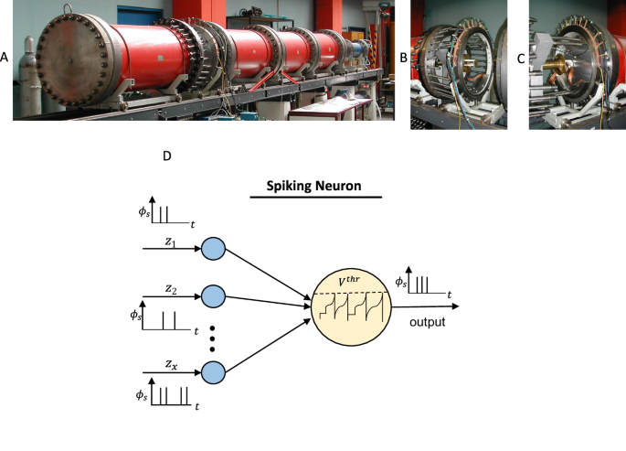
A Experimental set-up for transient signals, (B) short-time measurement devices, (C) positioning of a sensor for solid deformations at the open shock tube for calibration, (D) principle of spiking neuron.

Full size image

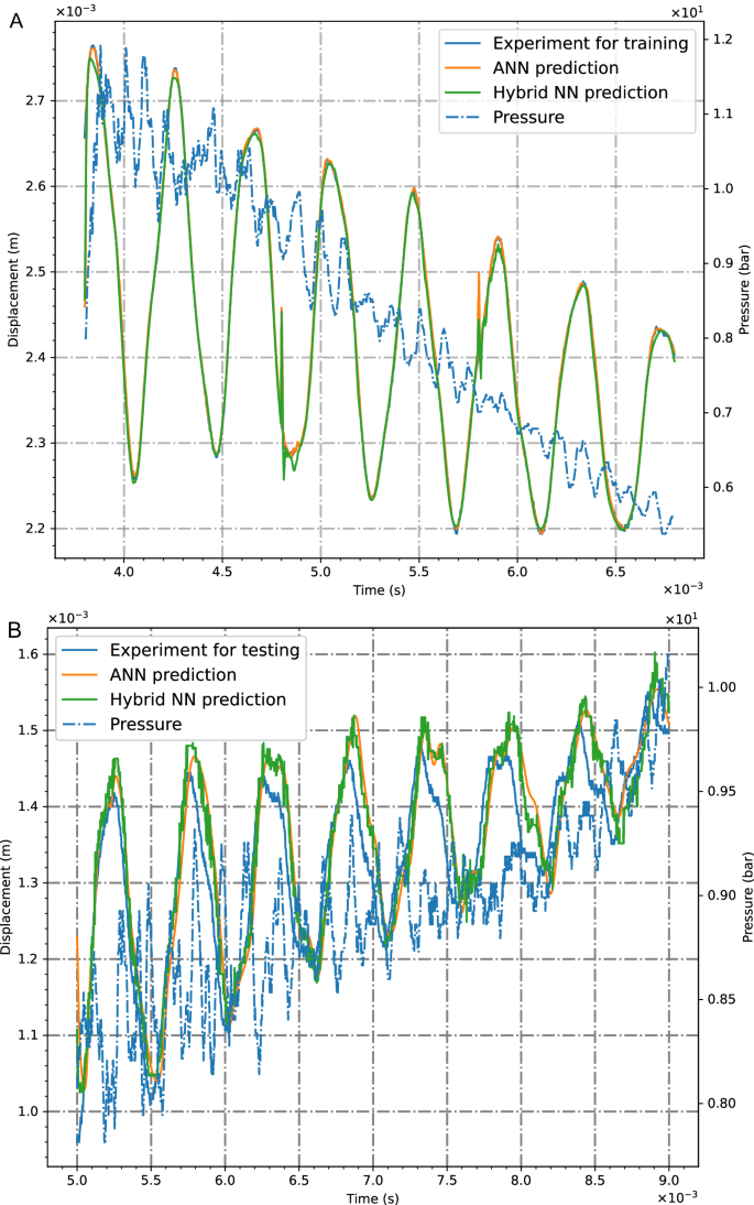
The evolution of pressure and deformation signals, measured during the shock wave duration representing non-harmonic transient functions, are illustrated in Fig. 2. Furthermore, results obtained with trained networks (Fig. 2A) of the second and third kinds are shown, while the pressure, wave propagation speed, and specimen’s properties are used as input quantities and the structural deflection as an output signal. In the legend, both cases ANN (second generation only) and hybrid prediction (third and second generation) are shown for training and leading to good agreements with measurements. As precisely shown in the following neural network architectures, we introduce hybrid networks to be composed of ANNs and SNNs combining advantages of both types of networks. The hybrid SNN/ANN approach in Fig. 2A computes better the oscillations at the end of the time interval than the ANN does. The extrapolation capabilities are demonstrated in the validation study in Fig. 2B. Again, the results using the third-generation network turn out to be closer to the measurement. Data-driven neural networks are known to exhibit a small range of extrapolation capabilities. However, in the present framework, we enhance the network’s prediction opportunities by making use of the inherent path dependence of SNNs. Following this intention, not only single input pairs are passed through the network, but sequences composed of ordered pairs of values are applied immediately at the input layer in Fig. 1D. This kind of data preparation (see Methods) including the physical path-dependency, is embedded into the inherently time-depending spiking neurons, and, hence, allows it to outperform the prediction of path-dependent transient signals beyond the trained data. In other words, by making use of the time-dependent nature of SNNs, the prediction capabilities of a regression framework can be improved compared to traditional ANNs.

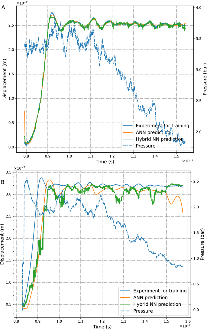
Measurements and calculations with second-order ANN and third-order hybrid neural networks for (A) training and (B) validation.

Full size image

Encoding strategies and nonlinear regression framework

The encoding principle plays a key role in regression analysis with SNNs. Here, the need for a systematic transformation between real-valued and binary signals is more pronounced as in classification studies, where e.g. image representations can directly be regarded as binary values diminishing the need for encoding strategies. Once a sufficient training result is established for second-generation networks, a validation study can lead to sufficient correlations between measurement and predictions, see Fig. 2B. However, since the SNN works with sparse spike train signals, physical input values have to be encoded towards binary quantities. Encoding strategies are reported in literature^43,50 and play a crucial role in training SNNs, especially for regression tasks. In Fig. 3, different principles are shown. For classification problems, rate-encoding can be adopted, accounting for the high intensity of pixels leading to the firing of spike trains. Alternatively, the latency encoding and latency-coded decoding methods decide when a spike appears depending on the pixel’s intensity. In delta modulation, the spike firing depends on the positive gradient of the input data. However, the present study intends to propose an encoding method that is appropriate for a broad spectrum of neuromorphic chips such as Loihi or SynSense Xylo and Speck. For this reason and the aim of non-linear regression, a machine-learnable transformation of real physical values to spike representations is conducted by the first SNN layer, see Fig. 4. Following this autoencoding principle, learnable parameters in the first layer are adapted for this transformation process accounting for path- and time-dependent signal evolutions. Due to the fact that spiking neurons are inherently time-dependent, the propagation of spikes through the network has to run synchronously to incoming real-valued signals denoting the deformation history of the considered structure. This is a constraint that occurs during a function approximation of dynamic solid deformations. The autoencoding strategy in Fig. 4 maps real values to spike trains causing internal neuron voltage evolutions in the whole network. Here, we face a time- and path-dependent process with real physical times, which is typically in nonlinear regression problems. For this reason, the time scale in spike trains must fit the time passed during a structural deformation process. Following this line of reasoning, one real physical sequence is mapped to a binary sequence for the same time interval.

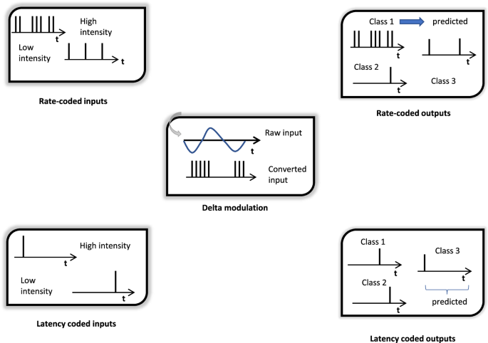
Rate, latency, and delta modulation procedures reported in the literature.

Full size image

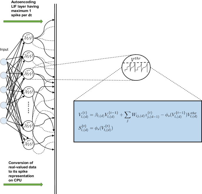
Real-valued signals are converted into binary values in the case of LIF neurons.

Full size image

However, in contrast to deep learning techniques of 2nd generation neurons, no activation functions such as e.g. sigmoid are applied in the spiking neuron. Instead, the neuron’s membrane potential and, hence, its ability to send spike signals are covered by an ordinary differential equation. The most popular one is the Leaky-Integrate-and-Fire model, which is applied in the present work as a first step to develop it further to a spiking variant of a Legrendre Memory Unit. This intention is motivated by the need for a high amount of memory in the nonlinear regression of complex transient signals.

Firstly, after adopting the autoencoding strategy for the input layer and the first SNN layer (Fig. 4), we proceed with the sparse signal voltage processing to subsequent feed-forward layers. In a further step, the LMU is added for higher memory access.

Assuming an arbitrary number of hidden layers, the voltage representation in Figs. 1D, 4 can be developed further in component form for each hidden neuron. Starting with a voltage V_t at a certain time t, the output of a neuron ℓ from an arbitrary hidden layer d of an SNN at time t can be written as

with ϕ_s representing the spike activation when a voltage threshold ({V}_{ell ,(d)}^{thr}) is exceeded

Here, the membrane potential of the neuron is expressed by ({V}_{ell ,(d)}^{t}), weights are stored in W_(d), β_ℓ,(d) stands for the membrane decay rate, and ({{{{bf{z}}}}}_{d-1}^{t}) is the output of the precedent hidden layer. Hence, the learnable parameters of the transformation are

Thus, the spiking neuron includes a membrane potential and once exceeding the threshold, an activated signal of 1 is passed while the potential is reset, using the term ({phi }_{s}({V}_{ell ,(d)}^{t-1}){V}_{ell ,(d)}^{thr}), else an activated output of zero is passed to the next layer. This principle of binary and sparse signal processing makes the SNNs so efficient concerning less energy consumption on neuromorphic chips. The memory and synaptic weights are accessed only when a spike appears. On the contrary, 2nd generation networks use matrix multiplication and communicate through dense signals.

Since the machine-learning process involves backpropagation as well, the discontinuous nature of spikes has to be overcome. Following the method of surrogate gradients^31,51,52 we prepare the SNN by an arcus tangent activation surrogate proposed in^42,51 for a backward pass with differentiable spike representations.

Spiking legendre memory units for non-linear regression

The LMU approach as an alternative spike activation compared to LIF enables us to separate the network’s architecture and the accessible memory from each other. This is an important attribute for the path-depending nonlinear regression since the memory provides the necessary set of parameters, in which long and short-term events are stored. The advantage of memory access was described and proofed in works of^44,47.

In Fig. 5, the result of the developed multilayered spiking variant of the Legendre Memory Unit (LMU)⁴⁷ is shown, acting as unit cells inside the SNN architecture. With the combination of sparse spiking signals and LMU cells, substituting activation functions of second-generation networks, nonlinear regression with time-dependent complex transient signals becomes possible in the present study. However, for a better comparison, we also equip the second-generation counterpart with LMU.

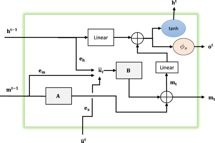
The memory variable is denoted by m(t) depending on time t. Memory and vector u_t contribute to matrices (A, B) resulting in additional parameters in e_x, e_h, e_m. The output for the following time step is h^t and o^t for the spike output of the whole sequence.

Full size image

Alternatively, the spiking neurons to be enhanced by high memory access for nonlinear regression can also be derived with LSTM cells. However, an alternative approach of spiking variants of LSTM units is not followed here, since their memory is coupled to the number of hidden neurons. The memory of an LMU cell is not stored like in an LSTM cell⁵³ and is, therefore, independent of the number of hidden neurons initialized in a layer and is instead initialized through an ODE that approximates a linear transfer function for a continuous delay⁴⁴, see Fig. 5. Since the memory capability is connected to the number of free weights, the LMU approach cares for the available set of parameters and does not require an extension of the network’s architecture. This attribute enables the LMUs to perform equivalently-sized LSTMs during long periods⁴⁴. We make use in this approach of the dynamic computation of the LMU cell’s memory m^t by starting from the linear transfer function for the continuous delay and approximating the memory by n coupled ordinary differential equations (ODEs)⁴⁴ expressed by

where m(t) ∈ Rⁿ represents a state vector with n dimensions, (A, B) represent ideal state-space matrices derived from the Padé approximants as mentioned in studies^44,54, and u(t) ∈ R represents an input signal which is orthogonalized across a sliding time window of length θ. These n sets of equations are mapped to the memory of the cell at discrete time steps t and are expressed by

where (tilde{{{{bf{A}}}}}) and (tilde{{{{bf{B}}}}}) are discretized matrices and are computed here using the zero-order hold (ZOH) method. The vector u^t writes to the memory in Eq. (5) and is computed by using the equation

The expressions e_x, e_h, e_m are treated as parameters dynamically projecting relevant information in its memory cell, and x^t denotes the input fed into the model. In a final step, the memory is passed to a recurrent hidden cell nonlinearly transforming the memory to finalize the output o^t for the whole data sequence and the output for a time step t with h^t to be equal

and

with bias b. The spiking variant of the LMU cell (SLMU) can be computed by keeping the Eqs. (4), (5), and (6) unchanged and introducing the spikes in Eqs. (7) and (8) leading to

with j, and k representing the number of total units of neurons from the current layer and the memory. Also, ϕ_s represents the spike activation in the form

Finally, a decoding strategy has to be introduced for re-transforming spiking signals to real physical values at the end of the forward pass, see Fig. 6A. Here, a recurrent variant of the spiking neural network (SRNN) is used to decode the binary spikes, with the potential to perform outputs in real values rather than the spikes⁴². A recurrent principle is used here since it requires less energy than the LMU variant. This transformation process follows the expression for the voltage

with an additional set of recurrent weights denoted by U_(d) and where j and k denote the total number of units from the previous layer and current layer, respectively. Other strategies for encoding and decoding between spikes and physical values can be found in⁵⁵. In the present investigation, spiking and non-spiking variants need the same number of transformations, however, to introduce robustness in the prediction of the non-spiking variant and avoid overfitting, a dropout operation⁵⁶ specific to the non-spiking variant is introduced as shown in Fig. 6B. The spiking variant inhibits an inherent dropout operation to be discussed in the following subsections.

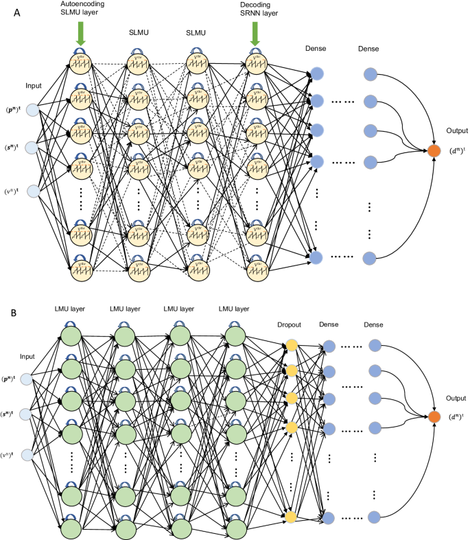
A Hybrid spiking and dense network with autoencoding and decoding layer. B Dense artificial neural network with drop-out layer.

Full size image

SNN and ANN architectures with hyperparameters

In Fig. 6, the finally obtained third-generation neural network and its second-generation counterpart are presented. In Fig. 6A, the SNN together with densely fully connected layers and input and output layers leading to a so-called hybrid model is shown. Sparse signal processing is indicated by dashed arrows while solid arrows denote suddenly occurring spike transmissions. While the second generation neuron receives real-valued inputs and uses the weighted sum as a criterion for an output signal, the spiking neuron is submitted to spike train signals leading to a time history of the voltage evolution and triggering the spike train output of the neuron as described in Eqs. (1), (2), (9), (10), (11) and in Figs. 1D, 4.

The input layer includes measured values denoted by neurons of the second generation. A number of three input values is illustrated. The real-valued signals are converted into binary signals by an autoencoding strategy using the first SNN layer for transforming physical data into spike representations. During the propagation of signals and time sequences, solid and dashed lines would always alternate depending on each spike train in between all spiking neurons. This fact gives already an impression of the remarkable energy efficiency compared to the second-generation model in Fig. 6B. There, all dense neuronal connections are always active independently on the time leading to a much higher energy consumption. However, before the data preparation and energy consumption are discussed in the following subsections, it can be concluded that the final architecture of the hybrid model is prepared with all the following attributes. An input layer with measured pressure ({left({p}^{n}right)}^{t}), a specimen’s property ({left({s}^{n}right)}^{t}) denoting the ratio between Young’s Modulus and diameter, and the shock wave velocity ({left({v}^{n}right)}^{t}), see also²⁸. The superscripts ()ⁿ and ()^t stand for normalised values and time, respectively. The output layer includes only the specimen’s deformation ({left({d}^{n}right)}^{t}). The first SNN layer enables autoencoding, while the last SNN layer is used for decoding spikes to real-valued signals by using a spiking recurrent neural network expressed by Eq. (11). In-between auto- and decoding areas, a variable number of hidden layers can be created. After encoding, a set of dense layers can also be added if necessary e.g. for the training process. However, each dense connection needs more energy than the SNN communication, so this hybrid composition must be chosen carefully concerning the intended sustainability.

During the training of the described neural network models the number of SLMU layers, the number of hidden units in the SLMU layer, the number of units of the SRNN layer, the number of memory units of the SLMU layer, the number of hidden dense layers, the number of dropout percentage, and the number of units of the dense layers are determined and shown in Table 1. A Hyperband search algorithm⁵⁷ for efficient exploration and investigation of suitable architectures as well as Adam optimizer’s learning rate (ζ = 0.001) and its exponential decay rates β_e1 = 0.9 and β_e2 = 0.999 were applied. As a comparison in Fig. 6B, the alternative second-generation neural network is presented, working with dense connections, only. To account for regulation effects, a drop-out layer is used here, which is not necessary for the SNN counterpart due to the brain-inspired regularisation in the present nonlinear regression as described below.

Nonlinear regression of complex transient signals

In Figs. 7–9 the SSN model vs. the ANN counterpart are verified for other loading histories and specimen properties. In Fig. 7 two examples are shown, in which both third and second-generation networks lead to good training results, while in Fig. 9 also validation results are shown. The transient data in short-time scales is gained by an experimental set-up with an experimental procedure equivalent to the one in Fig. 1 but using different specimens and pressure histories as it is visible in the diagrams. This ensures a mostly general approach in the present investigation. The set-up is decomposed in Fig. 8A–D into its details for measuring solid deformations and pressures leading to the recording of deflection and pressure signals in Figs. 7, 9. In Fig. 9B, the prediction is tested with the trained networks of Fig. 7B for steel, and a good agreement with the measurement is achieved. This observation continues in Fig. 10A, where four subsequent impulsive pressure loads are performed, causing complex deflection histories of the specimen. However, both types of networks can outperform the signals with a deviation at the end. However, to investigate the extrapolation capability after training of three loading steps, the fourth one is predicted by the SNN and ANN networks. In Fig. 10B, the green and indigo curves correspond to the response over the validation sequences highlighting that the model has learned the nonlinear evolution and can be deployed for further extrapolation beyond the training data. Even though the external loadings during the validation sequences are beyond the training data, the model behaves less sensitively towards sequence development. This indicates that with the proposed autoencoding strategy an SNN model was developed, which is as accurate as the second-generation model.

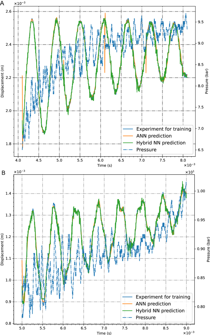
Training of 3rd and 2nd generation networks with (A) copper and (B) steel material.

Full size image

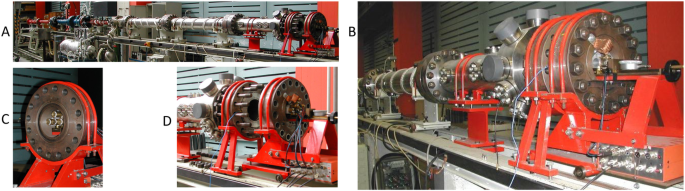
A Set-up for steel and copper specimens, (B) measurement adjustments for short-time pressures and deformations, (C) displacement sensors, (D) open tube for calibration.

Full size image

A Training with steel material, (B) validation with steel material.

Full size image

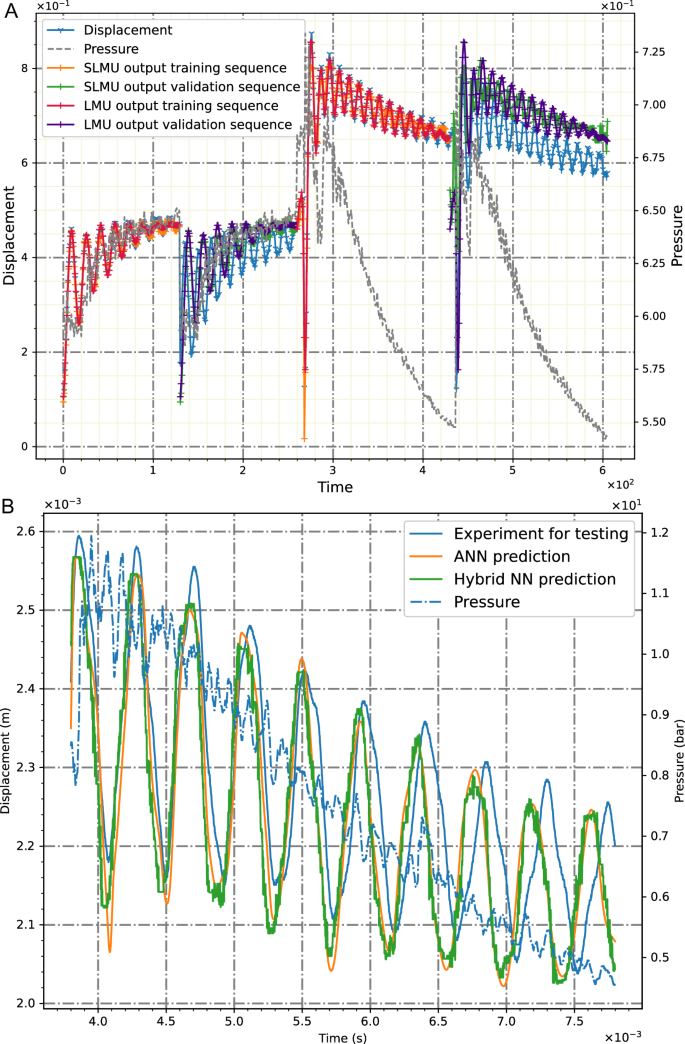
A Training and validation with steel under repeated loadings, spiking LMU with hybrid model and LMU with ANN, (B) validation with steel material.

Full size image

Due to the described network models with path dependency and high memory access, both networks have learned the underlying nonlinear evolution of the output signals and perform, with a deviation, the oscillating behavior. Furthermore, another extrapolation capability of the networks is investigated in Fig. 10B with data beyond the training range used in Fig. 9A. The subjected pressure is slightly different from the one in Fig. 9A but leading also to good agreements with the measurement.

Accuracy and brain-inspired regularisation

In Table 2, the accuracy of the calculated signal evolution compared to the measurements is presented taking RMSE values into account. In the first column, T and V denote, if the neural network computing was used for training or validation, respectively. The accuracy of computing the measured signals is summarised in Table 2, where the RMSE values indicate an acceptable correlation to the measurements. However, due to sparse binary communications between spiking neurons, in the present study, the training time is longer than that of the second-generation counterpart. To find a compromise between training duration and energy need, the hybrid approach as shown in Fig. 6A is proposed, in which only the layers that consume the most energy, in this case, the LMU, are converted into their spiking variant (SLMU) and combined with dense transformations to predict nonlinear behavior. Following this strategy, a better convergence rate while training the hybrid SLMU model is obtained. Furthermore, validation experiments are performed and a stable response for these experiments highlights that both models have not only memorized the data but have identified the trends of the physical evolution. One aspect can be in this case the dropout transformation and the spiking mechanism deployed in the LMU and SLMU models. The observed effect of an inherent drop-out during regression with the SNN should be highlighted as well. In the SNN, a neuron is activated only when the threshold potential (V^thr) is exceeded, else it remains deactivated. Hence, during a forward pass only a certain amount of neurons fire the spike trains. A similar behavior happens when a dropout⁵⁶ layer is added after a second-generation layer, wherein a subset of neurons is set to zero with a certain probability. Consequently, we can conclude an inherent brain-inspired regularization occurs in spiking neurons.

Energy consumption

Even though the 2nd generation model performs similar results as the 3rd generation one, the neuromorphic network leads to significantly lower energy consumption than the 2nd generation topology. To quantify these energy savings, a power profiling with different processors is carried out in Tables 3, 4 representing the consumed energy during one forward pass. To trace the energy consumption throughout the networks, in Table 3, the energy values are shown for each layer separately. Due to the hybrid network architecture, the comparison takes place between CPU, GPU, Loihi, Loihi (SLMU layers) + GPU (Dense layers), and Loihi (SLMU layers) + CPU (Dense layers). The total energy denotes the one required to perform all synaptic operations and neuron updates. It should be mentioned that the energy cost for deploying the model on/off the device is not included here. All energy values are determined with KerasSpiking^33,58. Due to their sparse connections, the memory and neurons are accessed only when the threshold is exceeded, initiating synaptic operations only for activated neurons. This effect has a dominant influence on the energy consumption of the network during signal processing on a Loihi chip, see Tables 3, 4. The smallest energy consumption is obtained with a third-generation model on a Loihi chip. Each part of the framework does not save energy. Only those parts being deployed on the neuromorphic chip having spiking transformation save energy. In Table 4, the reduction factor is shown for the energy needed by a conventional processor in relation to the neuromorphic chip or a hybrid composition. A significant energy saving by the ratio of classical computing using CPU and GPU to the new approach with third-generation SNNs can be observed due to reduction factors of 1176.33 and 35581.4 (see Table 4). The results are determined while comparing the energy of the spiking variant being deployed on the Loihi chip with the non-spiking variant on the GPU and CPU. However, KerasSpiking assumes that the deployed NN model consists of only third-generation neurons. The energy values corresponding to the second-generation dense layers do not represent the actual values for the proposed hybrid model. Since sustainable computing by SNNs is required in this study, the relation between spiking and dense layers plays a crucial role in keeping overall energy saving for the entire network. A reliable set of values can be obtained by deploying only the SLMU layers on the Loihi chip and the dense layers on GPU/CPU as shown in Tables 3 and 4. Hence, a total reduction factor of 21.2775 and 1663.878 per epoch can be expected in comparison to the second-generation counterpart.

In the present study, a nonlinear regression framework for spiking neural networks on neuromorphic processors is proposed and its sustainability in the form of significant energy saving is demonstrated. However, a crucial point for triggering the spiking neurons is the encoding between real physical and binary values, which was, here, introduced by autoencoding with the first spiking layer. To keep the energy consumption during decoding as small as possible a recurrent spiking layer was introduced. Additional dense connections can be introduced for improving convergence, however, then already gained energy savings could be reduced. Consequently, the developed hybrid neural network model accounts for several attributes such as energy saving, reduced training loss due to a hybrid solution, and encoding strategies. Moreover, due to their inherently recurrent nature, the SNNs offer themselves for path-dependent regression tasks, which must be implemented in second-generation networks more circumstantially by recurrent loops. Here, sequential data is used to account for the SNN’s advantage of time dependency in function approximation. The SNNs are also appropriate to further enhance them by additional Legendre Memory Units (LMU) independently of the network architecture. The LMU acts in the single neuron with additional memory, which is important for storing evolutive processes in path-dependent functions. To obtain complex transient signal processing in hybrid neural networks, experimental data was used being recorded by short-time measurement techniques in shock tubes leading to wave propagation phenomena in solids.

Data acquisition

In Fig. 11 the data acquisition for the data-driven neural network approach is described. The principle of a shock tube is shown in 11A consisting of a high-pressure chamber (HPC) and a low-pressure chamber (LPC) separated by a membrane from each other. The membranes presented in part B of Fig. 11 can consist of Hostaphan or Aluminum depending on the desired burst pressure. In the case of Hostaphan for pressures up to 15 bar a flange with an additional cross is inserted in the tube (see Fig. 11B) to avoid too early ruptures of the membranes. Aluminum membranes (Fig. 11C) include a cross on their surfaces causing a controlled opening of the membrane with pressures up to 30 bar avoiding that parts of the membrane tear up and move together with the shock wave. In the principle drawing (Fig. 11A) PCB 113A26 piezoelectric pressure sensors (PS) are located in flanges being able to measure fast pressure changes in rise times of 1 μs and are calibrated until 34.5 bar. Due to the conical shape of the tube between LPC and HPC, the pressure of the shock waves caused by the ruptured membrane is up to 7 bar in the LPC. A solid plate specimen is clamped at the end of the LPC being subjected to a plane shock wave front reflected at the specimen and propagated back through the shock tube. In this way, the pressure steps in the diagrams in Fig. 11D, E are caused. By varying the type of gas in the HPC different peak pressures and pressure evolutions, acting on the specimen, can be obtained, see Fig. 11E. To measure inelastic deformations of specimens in the tube during the impulse duration, a capacitive sensor, developed in^48,49 is located in front of the specimen’s center. Control devices next to the sensor are used to calibrate the sensor and to conclude from voltage signals on displacement quantities. All measured data is recorded with 1MHz sampling rate. To vary materials and geometry, the data of steel and copper specimens in an additional shock tube, shown in Fig. 8, is also used for data acquisition. Data collections of these experiments can be found in^10,48,49.

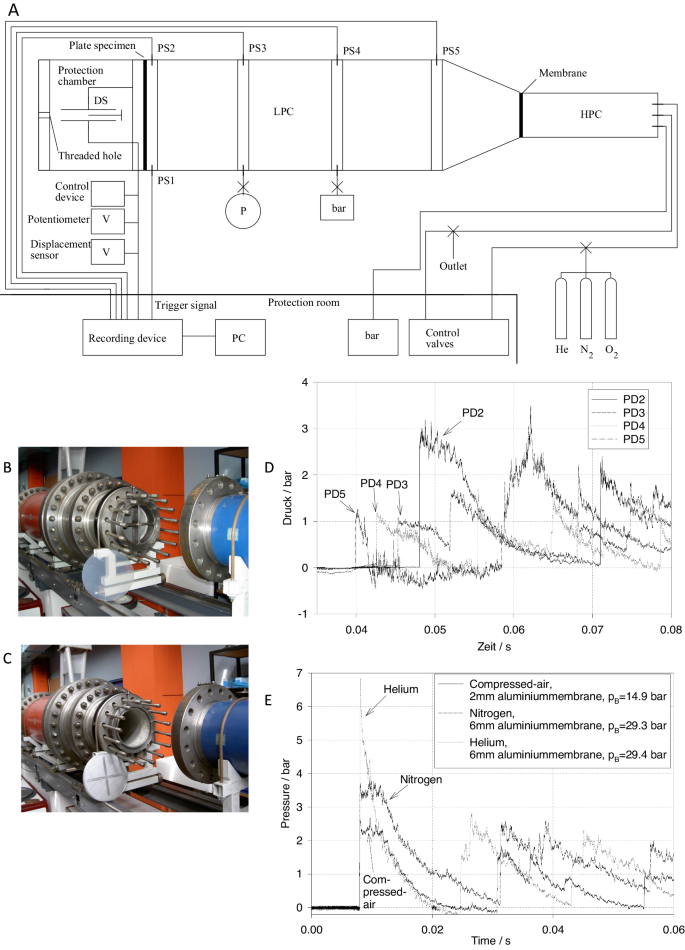
A Functionality of experimental set-up, data measurement, and recording, (B) mounting support with additional cross for Hostaphan membranes, (C) aluminum membranes with milled cross, (D) pressure signal triggering along the tube, (E) different pressure histories acting on the specimen.

Full size image

Data preparation

Here, data sequences instead of single pairs of data are prepared for training and validation. Following this procedure, it is made use of the inherently time-dependent property of spiking neurons. This technique is beneficial for all these purposes where path-dependent input and output variables are incorporated. To prepare the measured data for the neural network training, a sampling strategy with measurements that run over 15000 time steps is introduced. Generating a stack of experiments means analysing sequences with 500 time steps, hence, the input and output vectors include sequences with 500 data points each. They are extracted by a windowing technique, sliding with 500 time-steps over the measurements to collect the necessary training data. A stride of 500 steps is used during the training process to avoid any flow of redundant information. Following this strategy, a total of 100 sequences were extracted. Furthermore, a set of experiments is used to demonstrate the proposed model’s ability to adapt to previously unseen data.

Three input variables are chosen for the neural networks, the pressure p acting on the plate during the impulse period, the stiffness relation s denoting the relation between Young’s Modulus and plate diameter, and the shock wave velocity v. Hence, used notations for each sequence are ordered for the m^th sequence by a superscript (m), the i^th step in a sequence is denoted by superscript i, an input sequence is represented as

with a total number of I sequences. The output sequence denotes the specimen’s midpoint displacement y^(m). Input and output sequences have to be scaled to avoid convergence issues during training, which is ensured by a linear transformation following Min-Max standardization⁵⁹ in the form

In Eq. (13), η_max and η_min stand for maximum and minimum values of each feature and Eq. (14) maps the features to be in the range of [ − 1, 1]. Thus, the scaled ordered pair of input and output sequences are represented by ({[{{{{bf{x}}}}}^{n},{{{{bf{y}}}}}^{n}]}^{(m)}).

Hardware capabilities

The inference corresponding to the amount of energy consumed is computed through KerasSpiking V0.3. 1 where the Intel i7-4960X chip is used as the CPU, Nvidia GTX Titan Black as the GPU, and the Intel Loihi chip³³ as the neuromorphic hardware for processing the third-generation networks.