Indirect non-linear effects of landscape patterns on vegetation growth in Kunming City

Introduction
Cities have become centers of human activity and fossil fuel consumption due to dramatic urbanization over the last 50 years1. Urbanization gives rise to a multitude of ecological and environmental problems, posing a threat to urban sustainability2,3. In light of these challenges, urban greenery has emerged as a nature-based solution to combat climate change and address urban issues by providing essential ecosystem services. These services include thermal environment regulation, CO2 emission and air pollution reduction, runoff retention and recreation4. Consequently, cities worldwide have implemented urban greening policies, such as China’s “national forest city construction” initiative5.
Vegetation growth plays a vital role in achieving sustainability goals amidst the implementation of urban greening policies. The effects of urbanization on vegetation growth can be categorized into direct and indirect effects6,7. Direct effects occur when urbanization transforms natural surfaces into built-up areas or involves tree planting initiatives8. Indirect effects are related to environmental factors, such as changes in air temperature, atmospheric CO2 concentration, water availability, air quality, and nightlight regimes9. Urbanization has both positive and negative indirect effects on vegetation growth. On one hand, urbanization can elevate temperature and CO2 concentration, potentially promoting vegetation growth by extending the photosynthetic seasons10. On the other hand, it can exacerbate climatic extremes and air pollution, which in turn negatively affect vegetation growth11. Therefore, cities must prioritize the urbanization-induced indirect effect on vegetation growth (UIE-VG) when implementing urban greening policies. A positive UIE-VG guarantees the long-term and stable provision of ecosystem services12.
Although numerous ground-based studies have observed a positive UIE-VG, these studies have limitations in terms of spatial scope, making it challenging to infer general patterns6. To address this gap, ref. 6 proposed a comprehensive framework using satellite data to quantify the direct and indirect effects of urbanization on vegetation growth over large areas. Subsequent studies have validated this methodology and demonstrated that urbanization may indirectly promote vegetation growth, partially offsetting the carbon loss resulting from direct green land loss13,14. However, the direction and extent of the UIE-VG show great spatiotemporal heterogeneity6,14,15,16. Zhang et al.16 reported that urban development intensity, population density, and background climate collectively influence the UIE-VG at a global scale. However, integrating these findings into urban landscape planning remains challenging because these findings neglect the effects of landscape patterns on UIE-VG at the local scale.
Landscape pattern refers to the compositions and configurations of landscape elements17. Previous studies have shown that urban environments affecting vegetation growth are largely dependent on urban landscape patterns. Several studies indicate that the expansion of built-up areas is related to the intensification of urban heat islands, urban dry islands, and urban pollution islands18,19,20, which in turn influence vegetation growth21. Conversely, increasing green land and waterbodies can mitigate these effects22. Furthermore, a complex nonlinear relationship exists between microclimate factors and landscape patterns, and this relationship can vary in urbanization23. However, the relationship between landscape patterns and UIE-VG has not yet studied.
In this study, the boosted regression tree (BRT) method was utilized to examine the contributions and the effects of landscape patterns on the UIE-VG in Kunming from 2001 to 2019. The objectives of this study are: (1) to analyze how the UIE-VG changed from 2001 to 2019; (2) to investigate whether the contributions of landscape patterns on vegetation growth varied in urbanization; and (3) to explore whether the responses of vegetation growth to landscape patterns have similar non-linear relationships in urbanization.
Results
The NDVI–UI relationship in urbanization
To evaluate the UIE-VG, the relationship between the NDVI (normalized difference vegetation index) and UI (urbanization intensity) was identified from 2001 to 2019. The results show that the UIE-VG shifted gradually from negative to positive as UI increased (Fig. 1). Specifically, in 2001, urbanization had a negative UIE-VG when UI was less than 0.56, but the UIE-VG became positive when UI exceeded 0.56. In 2010 and 2019, the threshold values were 0.62 and 0.25, respectively, where the UIE-VG changed from negative to positive. The cubic regression analysis revealed that the NDVI–UI curves were statistically significant (p < 0.05) for each year. Though the model is acceptable (Adjusted ({r}^{2}) > 0.5), some scatter points still existed, especially in the areas with lower UIs. This finding highlighted that, even at the same urbanization density, the magnitude and direction of the UIE-VG varied at the local scale.

Points are NDVI values for each sample point. The zero-impact (red) line indicates the direct effects of urbanization on vegetation growth. The actual fitted curves between NDVI and UI are represented by green lines. The UI values where the red and green lines overlap are represented by the black dashed lines. Negative effects (({omega }_{{rm{i}}} < 0)) would be presented by sample points or green lines shown below the red lines, and vice versa.
Spatial variations in the UIE-VG (({{boldsymbol{omega }}}_{{bf{i}}})) from 2001 to 2019
The spatial distributions of the UIE-VG from 2001 to 2019 are illustrated in Fig. 2. Overall, the results indicated that negative UIE-VG gradually shifted to positive UIE-VG, which intensified over time. In 2001, the western and northern regions of the study area were primarily positively impacted by indirect effects, whereas a spatial combination of positive and negative indirect effects was observed in developing regions such as the eastern and southern parts. Between 2001 and 2010, the old urban areas (northern parts) and the newly developed areas (southeastern parts) demonstrated an increase in positive UIE-VG. Additionally, there were more areas with negative UIE-VG in the southeast. Between 2010 and 2019, most negative UIE-VG in the southeastern parts was transformed into positive UIE-VG.
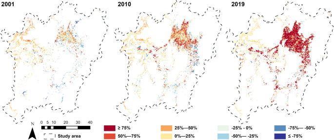
Growth enhancement and growth abatement are illustrated by the colors red and blue, respectively. Scale bar (1 km).
The results of the Welch t test showed significant differences in the mean ({omega }_{{rm{i}}}) across the years. Pairwise comparison of the average ({omega }_{{rm{i}}}) values was then performed using the Games-Howell test, and the results revealed a significant increase in the average ({omega }_{{rm{i}}}) in urbanization (Fig. 3). Specifically, the average ({omega }_{{rm{i}}}) in 2001 was 4%, indicating a slight UIE-VG when the city size was small. The average ({omega }_{{rm{i}}}) increased to 14% in 2010 and reached its highest value of 56% in 2019.
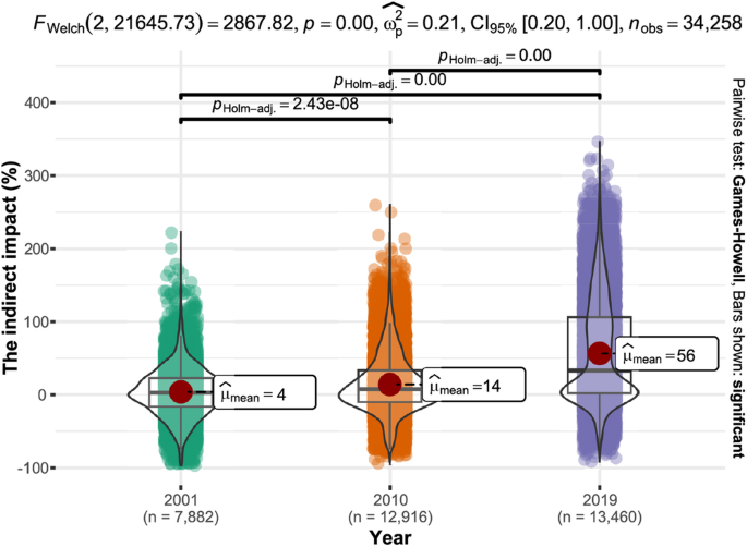
The results of the Welch t test are shown at the top. The results of the Games-Howell test are shown above the violin plot. The red points are the mean values of ({omega }_{{rm{i}}}). The bottom and up of the box indicate the first quartile (25%) and the third quartile (75%), respectively. The line within the box indicates the median of ({omega }_{{rm{i}}}).
The variations on the contributions of landscape pattern to UIE-VG from 2001 to 2019
The contributions of landscape metrics at the class level were quantified based on the BRT model, and the contributions of landscape composition metrics and landscape configuration metrics were compared (Fig. 4). The results demonstrated that the built-up land metrics played important roles in influencing ({omega }_{{rm{i}}}). The total contribution of built-up land metrics was larger in 2019 (86.4%) than in 2010 (71.9%) and 2001 (21.5%). Moreover, the dominant factors in 2001 were landscape metrics of waterbodies, with a total contribution of 37.2%. However, the total contribution of waterbody metrics was much lower in 2010 (2.6%) and 2019 (1.1%). The total contribution of unused land metrics was the highest (31.5%) in 2001, followed by 2010 (18.0%) and 2019 (9.1%). Generally, the landscape metrics linked to vegetated areas were the least influential. The total contribution of vegetated area metrics was highest in 2001 (9.9%), followed by 2010 (7.5%) and 2019 (3.5%). In addition, the total contribution of landscape composition metrics was higher than that of landscape configuration metrics in 2019, but the opposite result was shown in 2001 and 2010.
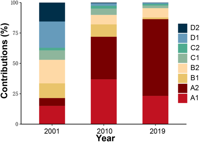
A, B, C, and D are built-up land, unused land, vegetated areas, and waterbodies, respectively. 1 and 2 represent configuration and composition metrics, respectively. The total contribution of all metrics is 100.
The contributions of the top ten landscape metrics are shown in Fig. 5. The results showed that the variations in ({omega }_{{rm{i}}}) were explained by the combined landscape metrics of different land cover types in the early stage of urban development in Kunming. However, built-up land metrics became major factors affecting vegetation growth in urbanization. In 2001, COHESION of waterbodies was the most influential metric (16.1%), followed by PLAND of unused land (12.3%) and PLAND of waterbodies (8.7%). The CA and LPI of unused land were less important, with contributions of 5.6% and 5.0%, respectively. The contributions of the other landscape metrics were less than 5%. In 2010, the most important factors were PLAND and LPI of the built-up land, with contributions of 32.1% and 25.5%, respectively. The COHESION of built-up land and PLAND of unused land were much less important, with contributions of 7.2% and 5.1%, respectively. In 2019, the most influential landscape metrics were PLAND and LPI of the built-up land, with contributions of 60.8% and 20.8%, respectively. However, the contributions of the other landscape metrics were much lower than 4%. The contributions of vegetated area metrics were always less than 2% in urbanization.
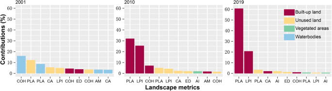
COH, PLA, and AM represent COHESION, PLAND, and AREA_MN, respectively.
The variations in the non-linear effects of landscape patterns on UIE-VG
The marginal effects and kernel distribution density of the three dominant landscape metrics for each land cover type are shown in Figs. 6–9. The marginal effects indicated the non-linear relationship between a single landscape metric and ({omega }_{{rm{i}}}) by controlling all the other variables at their average values. In general, ({omega }_{{rm{i}}}) was positively correlated with built-up land metrics. However, the unused land and waterbody metrics had a negative influence on ({omega }_{{rm{i}}}). In addition, both built-up land and unused land patterns had similar effects on vegetation growth in urbanization. However, there were significant differences in the non-linear relationships between vegetated area and waterbody metrics and ({omega }_{{rm{i}}}) from 2001 to 2019.
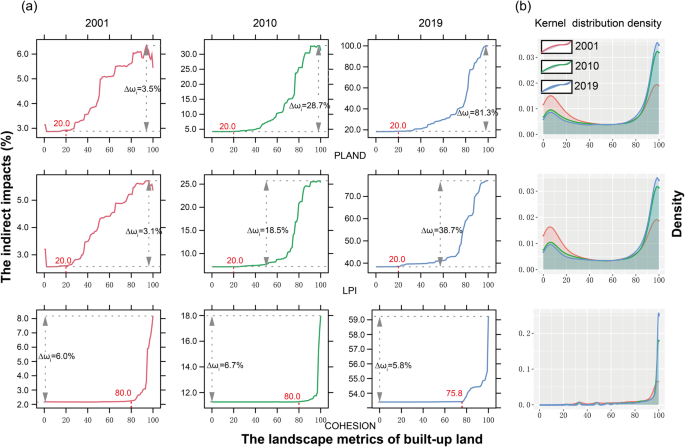
a The marginal effects of the three dominant landscape metrics of built-up land on ωi. ∆ωi represents the regulation amplitude of ωi. b The kernel distribution density of landscape metrics.
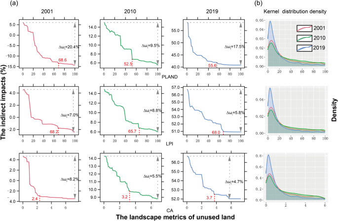
a The marginal effects of the three dominant landscape metrics of unused land on ωi. ∆ωi represents the regulation amplitude of ωi. b The kernel distribution density of landscape metrics.
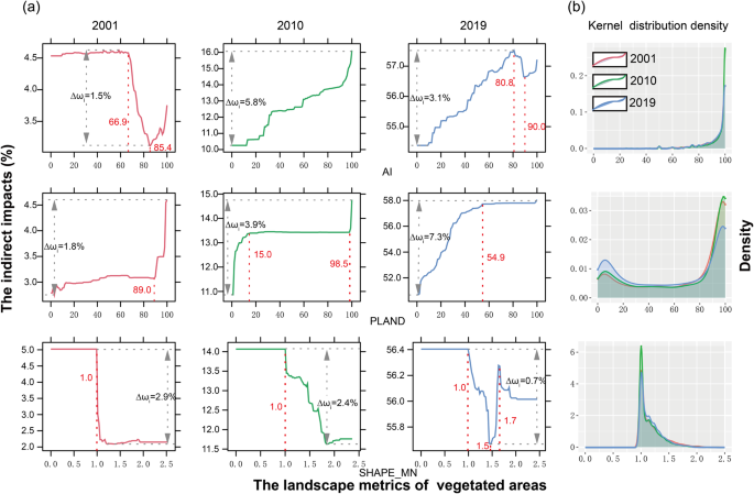
a The marginal effects of the three dominant landscape metrics of vegetated areas on ωi. ∆ωi represents the regulation amplitude of ωi. b The kernel distribution density of landscape metrics.
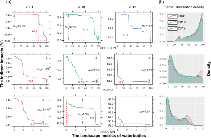
a The marginal effects of the three dominant landscape metrics of waterbodies on ωi. ∆ωi represents the regulation amplitude of ωi. b The kernel distribution density of landscape metrics.
Among the dominant built-up land metrics (Fig. 6), the values of PLAND and LPI were mainly distributed in the range of 80–100%, and the COHESION peak values were 100. In addition, compared to 2001, there were larger aggregated built-up patches in 2010 and 2019. PLAND, LPI and COHESION showed a positive influence on ({omega }_{{rm{i}}}), which indicated that large areas of aggregated built-up land enhanced the urbanization-induced indirect effects on vegetation growth. An exponential function relationship between built-up land metrics and ({omega }_{{rm{i}}}) was observed across years. However, the ({omega }_{{rm{i}}}) regulation amplitudes (({Delta omega }_{{rm{i}}})) for all built-up land metrics, except COHESION, were much higher in 2019 than the ({Delta omega }_{{rm{i}}}) in both 2010 and 2001. Moreover, the positive effects of increasing PLAND, LPI and COHESION on ({omega }_{{rm{i}}}) increased significantly when PLAND > 20%, LPI > 20% and COHESION > 80.
Among the primary unused land metrics (Fig. 7), PLAND, LPI, and CA exhibited a negative exponential correlation with ({omega }_{{rm{i}}}). Compared to 2001 and 2010, there were more sparse, small patches of unused land in 2019, according to the results of kernel density analysis. In addition, the regulation amplitudes of ({omega }_{{rm{i}}}) (({Delta omega }_{{rm{i}}})) for different unused land metrics varied across years. The ({Delta omega }_{{rm{i}}}) for PLAND in 2001 and 2019 was ~20.4% and 17.5%, respectively, which was larger than the ({Delta omega }_{{rm{i}}}) in 2010 (9.5%), whereas the opposite results were shown in the ({Delta omega }_{{rm{i}}}) for LPI. The largest ({Delta omega }_{{rm{i}}}) for CA was observed in 2001 (8.2%), followed by 2010 (5.5%) and 2019 (4.7%). Furthermore, the negative effects of increasing PLAND, LPI, and CA on ({omega }_{{rm{i}}}) declined as the values of unused land metrics increased, especially when the values exceeded the threshold presented by the red dashed lines.
The non-linear relationships between vegetated area metrics and ({omega }_{{rm{i}}}) varied from 2001 to 2019 (Fig. 8). According to the results of the kernel density analysis, the PLAND of the vegetated areas was larger in 2001 and 2010 than in 2019. Compared to 2001 and 2019, there were more clumped and complex-shaped patches of vegetated areas in 2010. In addition, the ({Delta omega }_{{rm{i}}}) values for all dominant vegetated area metrics were less than 7.3% from 2001 to 2019. When AI was between 66.9 and 85.4, the increase in AI showed a negative impact on ({omega }_{{rm{i}}}) in 2001. However, in 2010 and 2019, there was a positive relationship between AI and ({omega }_{{rm{i}}}). ({omega }_{{rm{i}}}) was positively impacted by PLAND across years, but the patterns of fitted curves changed. When SHAPE_MN > 1.0, SHAPE_MN was negatively correlated with ({omega }_{{rm{i}}}) in 2001 and 2010. The same results were shown in 2019 when SHAPE_MN was between 1.0 and 1.5. However, the increase in SHAPE_MN had a positive impact on ({omega }_{{rm{i}}}) in 2019, when SHAPE_MN was between 1.5 and 1.7.
For waterbody metrics, high values of COHESION, PLAND, and AREA_MN showed a low ({omega }_{{rm{i}}}) (Fig. 9). The kernel density results indicated that the waterbody patches were larger and more clumped in 2001 than in both 2010 and 2019. In 2001, the ({Delta omega }_{{rm{i}}}) for COHESION, PLAND, and AREA_MN were ~20.6%, 11.8%, and 6.4%, respectively. However, the ({Delta omega }_{{rm{i}}}) values for all main waterbody metrics were less than 4.7% in 2010 and 2019. When COHESION > 31.5, a sharp decrease in ({omega }_{{rm{i}}}) was observed in 2019. Similar patterns occurred when the COHESION values in 2001 and 2010 were higher than 67.9 and 74.4, respectively. In addition, when the PLAND values in 2001, 2010, and 2019 were larger than 58.3%, 54.5%, and 21.8%, respectively, the negative effects of PLAND on ({omega }_{{rm{i}}}) were reduced. AREA_MN had almost no effect on ({omega }_{{rm{i}}}) in 2010, when AREA_MN values ranged from 0.1 ha to 6.0 ha. The same results were observed when the AREA_MN values in 2001 and 2019 were greater than 4.6 ha and 1.2 ha, respectively.
Discussion
Urban greening is becoming an important strategy in improving living environment quality and urban sustainability5. Understanding how vegetation growth responds to urbanization can help in planning for urban greening aimed at providing sustainable ecosystem services. Although previous research has examined the inter-city factors driving UIE-VG, little investigation was conducted on the effects of urban landscape patterns on UIE-VG at the local scale. This study quantified the spatiotemporal evolution of UIE-VG and the relationships between landscape patterns and UIE-VG during the urbanization of Kunming City.
To better understand how urban environments affect vegetation growth, it is vital to distinguish the direct and indirect effects of urbanization on vegetation growth6. While negative UIE-VGs have been observed in some temperate and hot cities, several studies have reported extensive positive UIE-VGs13,16. The average UIE-VGs varied among cities and can range from −11.6% to 479.3%6,13,14,16,24,25,26. Our findings demonstrated that the average UIE-VG increased from 4 to 56% during the urbanization of Kunming City, which is consistent with most studies7,15,16. This indicated that enhancement on UIE-VG compensated for about 4%, 14 and 56% of the reduced productivity due to green land loss. However, some studies suggest that the trend of growth compensation will remain stable when the controlling factors of the UIE-VG reach the thresholds13,14.
In addition to quantifying the average UIE-VG, our study revealed significant variations in UIE-VG at the local scale, particularly in low urbanization areas. That is because a high landscape heterogeneity and fragmentation may exist in the low UI areas other than in the high UI areas, leading to more complex urban environments27. The uneven distribution of UIE-VG may lead to inequalities in the provision of ecosystem services and benefits by urban vegetation. This highlights the importance of considering not only spatial equity (vegetation coverage) but also quality equity (vegetation growth) in achieving urban green equity.
As hypothesized, the uneven UIE-VG at the local scale was mainly influenced by urban micro-environments, which are associated with landscape pattern28,29,30. The results of the BRT model indicated that landscape patterns provided better explanations for UIE-VG variations at the local scale. This suggests that rational urban landscape planning may enhance urban vegetation growth and help alleviate green inequity. In 2001, several types of landscape metrics, including built-up land metrics, waterbody metrics, and unused land metrics, jointly explained UIE-VG variations when the city size was small. However, built-up land metrics became the main cause of UIE-VG variations in 2010 and 2019, as evidenced by the increasing contributions and regulation amplitudes of built-up land metrics in urbanization (Figs. 4, 6). This indicated that the influence of landscape patterns on UIE-VG transitioned from joint control to the dominance of the built-up land landscape pattern as urbanization increased. First, the increasing influence of built-up land on thermal environments with the expansion of built-up lands has the potential to prolong the growing seasons of plants and increase the rate of plant physiological processes, leading to growth enhancement21. Second, the increase in anthropogenic heat flux and air pollution in urbanization is likely to have a beneficial impact on vegetation growth6,31,32,33 because higher concentrations of CO2 and N from pollutants can promote vegetation growth, which is referred to as fertilization effects34. Although high O3 concentrations may reduce plant growth26, some studies indicate that the spatial pattern of built-up lands has a negative correlation with O318, implying that growth enhancement might outweigh growth abatement regarding the effects of air pollution on vegetation growth26. Third, more large and aggregated built-up land patches were observed with urban expansion in Kunming (Fig. 6), which led to local warming in urban areas and could enhance vegetation growth. These findings suggest that urban planners should carefully consider the landscape patterns across multiple land cover types to enhance vegetation growth in the early stage of urbanization. However, the potential for enhancing vegetation growth through green infrastructure planning may be limited by urbanization.
The non-linear effect analysis revealed that landscape metrics related to area and aggregation for all land cover types were the main factors influencing UIE-VG. Furthermore, we observed a positive exponential response of vegetation growth to built-up land patterns, while an inverse exponential relationship was found for unused land patterns. For built-up land, previous studies have shown that large, aggregated built-up land can inhibit ventilation and absorb more solar radiation, exacerbating UHIs (urban heat islands) and air pollution18,19,35. Therefore, PLAND, LPI, and COHESION in built-up land had a positive effect on UIE-VG. For waterbodies, large waterbodies are generally believed to have a higher cooling effect than separate small waterbodies36. Additionally, artificial lakes can act as CO2 sinks due to autotrophic-based metabolism37. Consequently, large and aggregated waterbodies exhibited a negative correlation with UIE-VG. The unused land, typically covered with bare soil, had a negative correlation with UIE-VG primarily as a result of its high cooling efficiency through evapotranspiration and increased surface roughness38. It is notable that a complex nonlinear relationship between vegetated area metrics and UIE-VG was observed. This is because large areas of aggregated vegetation are resistant to anthropogenic disturbances and have been well managed in urban areas but also lower local temperatures and atmospheric CO2 concentrations22,39,40. Furthermore, based on the results of regulation amplitudes (({Delta omega }_{{rm{i}}})), built-up land landscape patterns significantly enhanced UIE-VG, with a range from 3.5% to 81.3%. Conversely, the landscape patterns of unused land and water bodies led to a decrease in UIE-VG, ranging from 0.7% to 20.6%.
In our study, areas with low urban intensities showed negative UIE-VG, which raises concerns regarding the sustainability and equity of urban greening initiatives (Fig. 1). Specifically, the turning point from negative to positive effects was significantly lower in 2019 (UI = 0.25) than in 2001 (UI = 0.56) and 2010 (UI = 0.62). Zhang et al.16 suggested that cities in developing countries, such as Beijing, might invest small resources in urban greening at the early urbanization stage, leading to negative UIE-VG. However, turning points were not observed in developed countries such as Paris16. Paradoxically, a study conducted in 32 major Chinese cities suggested that some cities with lower development levels than Beijing did not experience the turning point6. These contradictory findings indicate that differences in investment in urban greening across cities may not be the sole reason for negative UIE-VG in low urbanization areas.
To define the causes of turning point occurrence, sample points with UI values ranging from 0.25 to 0.60 were chosen to investigate the non-linear relationship between landscape pattern and UIE-VG using the BRT model (Supplementary Fig. 1 and Supplementary Table 1). We observed that metrics related to vegetated areas exhibited a consistently positive logistical effects on UIE-VG and high UIE-VG regulation amplitudes in areas with low urbanization (Supplementary Fig. 1), which differed from the outcomes obtained at the overall urbanization gradient level (Figs. 4, 8). This may be due to the weak cooling effect of vegetated areas in low urbanization areas41. Furthermore, compared to urban areas, rural areas tend to have more natural vegetation42, and large and aggregated vegetated area patches have higher diversity on natural populations and species, ultimately leading to higher vegetation productivity43,44,45. As shown in Supplementary Fig. 2, vegetated area patches in peri-urban areas were larger and more aggregated in 2019 than in 2001 and 2010, which resulted in a lower value of the turning point. These findings indicate that large and aggregated vegetated areas may mitigate the negative UIE-VG in low urbanization areas.
To better predict the carbon and water cycles of the earth system under future climate change, it is imperative to disentangle the linkages between UIE-VG and complex urban environments9. According to ref. 16 Urban development intensity, population density, and background climate collectively regulate average UIE-VG at a global scale. However, previous studies using coarse city-level sampling grains failed to fully capture the spatial heterogeneity of urban environmental factors within cities, thereby hindering the identification of non-linear relationships between UIE-VG and urban macro-environments46. For example, negative relationships between average UIE-VG and the UHI effect, represented by the temperature difference between urban and rural areas, were observed in Kunming, which is classified as a temperate region according to the Köppen-Geiger climate classification16. In contrast, our study found that built-up land patterns, which are positively correlated with urban temperature17, influenced UIE-VG variations at the local scale. Previous researches suggest that the urban-rural landscape classification alone cannot fully explain thermal contrasts within different urban patterns, leading to significant uncertainties in UHI calculations47. Therefore, we speculate that biased results in urban macro-environments affecting UIE-VG may be induced by the coarse spatial solution46. Since the unavailability on fine-grained datasets for studying the mechanisms of the UIE-VG at the local scale48, examining urban landscape patterns becomes critical in understanding the relationship between UIE-VG and urban micro-environments.
Exploring the non-linear relationships between landscape patterns and UIE-VG can provide evidence-based guidance for urban landscape planning to promote vegetation growth. For example, our findings demonstrate that the UIE-VG will not be affected when the percentage of built-up land was below 20%. Moreover, it is preferable for the built-up land patches to be clustered to meet certain criteria (COHESION > 80 and LPI > 20%, Fig. 6). Additionally, small and fragmented unused land patches exerted negative effects on UIE-VG. However, these negative effects stabilized when the PLAND, LPI, and CA of unused land exceeded certain thresholds (PLAND > 52.5%, LPI > 65.7, and CA > 2.4 ha, Fig. 7). Especially, we found that the large and aggregated vegetation areas mitigated the negative UIE-VG in low-urbanization areas. However, this effect became stable when the CA, PLAND, and ED of vegetation areas were greater than 3.5 ha, 54.1%, and 154.2, respectively (Supplementary Fig. 1).
Our results deepen understanding of the influence of landscape patterns on UIE-VG. These findings offer valuable insights to cities and policymakers on sustainable ecosystem services by urban greening. However, this study still has several limitations. First, given the lack of fine spatial images of controlling factors, a comprehensive influencing mechanism on how the interaction between landscape patterns and controlling factors affecting vegetation growth was not clarified. Second, the reasons for the higher value of the turning point in 2010 than in 2001 were unclear due to insufficient statistical samples with UI values ranging from 0.56 to 0.62. Third, further studies should consider the balance of multiple ecosystem services provided by vegetation, such as temperature regulation, in response to landscape pattern changes. Finally, differences in topographies and climate backgrounds may lead to diverse vegetation types that respond differently to a given set of environmental factors46,49,50. Therefore, future studies should focus on assessing how landscape patterns specifically influence UIE-VG across different topographies and climate backgrounds.
Methods
The study area
Kunming ((102^{circ} 10^{prime}) E–(103^{circ} 40^{prime}) E, (24^{circ} 23^{prime}) N–(26^{circ} 33^{prime}) N) is the capital of Yunnan Province, located in Southwest China, with an average elevation of 1900 m and a subtropical monsoon climate (Fig. 10). Over the past two decades, Kunming has undergone rapid urbanization, and this study specifically focuses on seven districts that have experienced significant growth. Before 2001, urbanization was mainly occurred in Wuhua, Panlong, Xishan, and Guandu Districts (Supplementary Figs. 3, 4). From 2001 to 2010, Kunming underwent a dramatic expansion of built-up lands, especially in Anning, Jinning, Chenggong and Guandu Districts, while intensive utilization of built-up land happened in the old urban areas. From 2010 to 2019, urbanized areas experienced further intensification and expansion. Considering the changes in landscape patterns that occurred during the rapid urbanization process, Kunming provides an ideal location for studying the relationship between landscape pattern and vegetation growth.
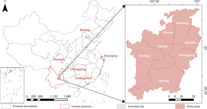
Scale bar (1 km).
Data sources
The land cover maps were generated using Landsat images with a supervisory classification to assess changes in urbanization density and landscape patterns from 2001 to 2019. For each year, cloud-free Landsat5/8 images were composited through the Google Earth Engine platform (GEE, https://developers.google.cn/earth-engine/). The classification identified five types of land cover: built-up land, cropland, unused land, vegetated areas, and waterbodies (Supplementary Table 2 and Supplementary Fig. 4). The training data were digitized in Google Earth according to the guidelines (https://www.wudapt.org/digitize-training-areas/). A random forest classifier was utilized for land cover mapping in ENVI 5.651. Accuracy was determined over 90% for each year, as evidenced by a confusion matrix (Supplementary Table 3).
Landsat NDVI time-series data (8-day composite) in 30 m were reconstructed using Gap Filling and Savitzky–Golay filtering method proposed by ref. 52 in GEE. To assess the overall state of vegetation growth for each year, we determined the average annual NDVI for each pixel using the GDAL package in Python 3.8.
Estimation of the effects of urbanization on vegetation growth
The effects of urbanization on vegetation growth were divided into direct and indirect effects based on the conceptual framework6. This study focuses on the UIE-VG. First, a linear relationship between UI ((beta)) and NDVI, often called a zero-impact straight line, can be used to show the direct effect of vegetation loss in urbanization. It can be defined as follows:
where ({V}_{{rm{zi}}}) represents each statistical unit’s theoretical NDVI, (beta) is the percentage of built-up land in each statistical unit, ({V}_{{rm{nv}}}) represents the NDVI value for nonvegetative surfaces, which was set to 0.05 because there is no vegetation activity below this threshold6, and ({V}_{{rm{v}}}) is the theoretical NDVI for each statistical unit with full coverage of vegetation.
({V}_{{rm{v}}}) can be defined as the intercept of the specific NDVI response curve to (beta) presented by a cubic polynomial model because high order (order > 3) can faithfully capture the relationship between UI and NDVI6,15:
where ({V}_{{rm{obs}}}) is the observed average annual NDVI.
Finally, the UIE-VG (({omega }_{{rm{i}}})) can be calculated as follows16:
({omega }_{{rm{i}}} > 0) indicates a positive indirect impact of urbanization on vegetation growth, and ({omega }_{{rm{i}}} < 0) represents a negative impact of urbanization on vegetation growth.
Calculation of landscape metrics
Based on previous studies on the relationship between the urban environment and landscape pattern, we selected ten landscape metrics, including total core area (CA), percentage of landscape (PLAND), mean patch area distribution (AREA_MN), mean shape index (SHAPE_MN), mean Euclidean nearest neighbor distance (ENN_MN), aggregation index (AI), patch cohesion index (COHESION), large patch index (LPI), patch density (PD) and edge density (ED) (Supplementary Table 4). The first three metrics define landscape composition, while the others examine landscape configuration. We calculated landscape metrics at the class level using the open-source “landscapemetrics” package in R 4.2.253.
Statistical analysis
For the analytical scale, a 250 (times) 250 ({{rm{m}}}^{2}) grid was chosen because it is of great relevancy for urban microclimate17,54. Farmland-covered statistical units were ignored due to the significant impact of agricultural activities. Moreover, based on ASTER GDEMV2 digital elevation model data (https://www.gscloud.cn/), statistical units with elevation sizes lower or higher than 50 m above the average elevation of the urban core were also excluded to prevent the effects of elevation differences on vegetation growth16. The “gbm” and “ggstatsplot” packages of R 4.2.2 were used for statistical analysis and graph creation.
To analyze the variations in UIE-VG, the distributions of UIE-VG between years were displayed in boxplots and violin plots. Welch’s t test was then applied to determine whether there was a significant difference among UIE-VG in different years. The Games-Howell test was used for pairwise comparisons of UIE-VG per year due to the rejection of the homogeneity test of variance and differences in sample size.
The BRT model, which combines the regression tree algorithm and the boosting method55, was utilized to calculate the contributions and the effects of landscape pattern on UIE-VG. The BRT model has been extensively utilized in studies of urban climate because it can capture complex relationships19,35. The parameters in the BRT model were n.trees (10,000), interaction.depth (9), shrinkage (0.001) and bag.fraction (0.5). The results of R-squared (({r}^{2})), root-mean-square error and mean error (ME) were derived after conducting a 10-fold cross-validation with 50 runs. The results of 10-fold cross-validation are shown in Supplementary Table 1 The average of ({r}^{2}) ranged from 0.5 to 0.7 ((p < 0.001)), giving good performance of the BRT model. Considering the sensitivity of landscape metrics to spatial scale, the performance of BRT model was estimated across multiple scales. The results showed that the BRT model showed better performance at the 250 m (times) 250 m scale compared to the other scales (Supplementary Fig. 5).
Reporting summary
Further information on research design is available in the Nature Research Reporting Summary linked to this article.


Responses