Open dataset of kinetics, kinematics, and electromyography of above-knee amputees during stand-up and sit-down

Background & Summary
Above-knee amputees have reduced mobility and quality of life compared to non-amputees. After the biological knee and ankle are removed, amputees are prescribed knee and ankle prostheses to replace these joints and provide support during activity1. A majority of currently-available knee and ankle prostheses are “energetically passive”, meaning they cannot provide net-positive energy to restore the biomechanical functions of the missing leg2,3. The lack of positive energy is especially detrimental during activities like stair ascent, stand-up, and ramp ascent. During these activities, above-knee amputees must compensate by overusing their prosthesis-side (residual) hip, their intact-side lower limb, and their upper body4,5,6. Compensatory movements, in turn, result in secondary health conditions such as back pain and osteoarthritis7. In addition, above-knee amputees may choose to participate less in society due to reduced mobility and fear of falling, leading to higher levels of depression compared to non-amputees8,9,10. However, the relationship between compensatory movements, secondary conditions, and mobility is poorly understood. Therefore, there is an unmet need for motion capture studies analyzing the biomechanics of amputees as they perform common activities of daily living.
Motion capture is a fundamental tool for clinical movement analysis, providing quantitative assessments of an individual’s kinematics and kinetics during activities. However, motion capture is resource-intensive, requiring expensive equipment, a large, dedicated space, access to subject populations, and experience and time to capture and process the data. Motion capture’s high cost of entry prevents many excellent researchers from contributing to the field of biomechanics.
Open-source datasets have the potential to expand access to biomechanical data, maximizing the clinical impact of expensive and time-consuming research studies11,12,13,14. Datasets allow researchers from around the world to test hypotheses and make comparisons without needing to collect and process the motion data on their own. Moreover, biomechanics datasets can be used by engineers to design assistive technologies, including lower-limb prostheses. Several biomechanical datasets have been published with healthy subjects performing activities such as walking, ramps, and stairs13,15 – most notably, the Winter dataset of healthy gait kinetics and kinematics14. Although healthy biomechanics provide useful references, datasets with clinical populations have a greater potential to inform clinical care and assistive technology development.
To the best of our knowledge, only two open datasets with lower-limb amputee participants have been published so far. The first is a dataset of 18 above-knee amputees walking at five speeds11. The second is a dataset of 14 above-knee amputees walking16. However, no open-access datasets have been published with above-knee amputees performing the sit-to-stand transitions. Standing up and sitting down are essential activities of daily living that able-bodied people perform about 60 times per day17. Without the ability to stand up and sit down, a person cannot get out of bed or use the restroom, which presents huge barriers to living independently. Standing up from a chair is especially difficult for above-knee amputees, whose passive prostheses cannot actively assist with the stand-up movement. Above-knee amputees compensate for the lack of energy from the prosthesis using unnatural and strenuous compensatory movements. However, the impact of these compensatory movements on their residual limb, contralateral leg, and upper body is largely unknown. To address this issue, we present an open biomechanical dataset with nine above-knee amputees standing up and sitting down while wearing their prescribed passive prostheses. This dataset has been used, in part, in two previous publications18,19. This dataset provides a unique resource for researchers and clinicians from a variety of disciplines, including ergonomics, occupational health, rehabilitation, and engineering. This dataset will enable researchers to explore the biomechanical effects of passive prosthesis use and design better prostheses and rehabilitation strategies to improve mobility, quality of life, and the standard of care for above-knee amputees.
Methods
Experiment and data collection
Subjects
This study protocol was approved by the University of Utah IRB (00103197, 6/16/2021). We recruited nine individuals with above-knee amputations. All of the subjects were K3-level “full community ambulators”. Inclusion criteria were unilateral above-knee amputation, daily use of prescribed prosthesis, and ability to stand up and sit down with or without the use of hands. Exclusion criteria included any musculoskeletal, cardiovascular, or other impairments that would prevent a subject from completing the study activities. Subjects provided written informed consent to participate in the study and consent for publication of videos and photographs. Subject demographics are included in Table 1. Data collection was performed in a single test session lasting less than four hours. The experiment comprised several steps, described below. Table 2 shows an overview of the steps of data processing, the contents of each folder, which types of variables are included, and any corrections performed. Table 3 shows the number of repetitions included in each step of data processing.
Equipment
We recorded the 3D locations of reflective markers using 12 Vicon “Vantage 5” cameras (Vicon Motion Systems Ltd; Oxford, UK) capturing at 200 Hz. We recorded forces using two in-ground AMTI OR6-7 force plates (Advanced Mechanical Technology, Inc; Watertown, MA, USA), capturing at 2000 Hz. We recorded electromyography (EMG) signals using Delsys Trigno Avanti sensors (Delsys Incorporated, Natick, MA, USA), capturing at 2000 Hz. We recorded video of every subject’s sit-to-stand trial using a Go-Pro Hero 5 video camera (GoPro, Inc; USA). We also recorded videos of some subjects using a Vicon Vue Video camera (Vicon Motion Systems Ltd; Oxford, UK).
The Vicon Vantage 5 cameras, the Vicon Vue Video camera, and the force plates were synchronized and recorded using Vicon Nexus 2 (Vicon Motion Systems Ltd; Oxford, UK). The EMG sensors were recorded using Vicon Nexus and were exactly synchronized with the Vicon cameras and force plates for every subject except TF01, whose EMGs were delayed by a constant number of frames (we corrected the delay in TF01’s EMGs in MATLAB). The Go-Pro was not synchronized – we manually started and stopped the recording at approximately the same time as the trial was started and stopped. For TF04, we started the Go-Pro video after the first stand-up. The placement of the Go-Pro relative to each subject is detailed in Table 1. Later, we deidentified the videos by blurring all of the faces using Adobe Premier Pro. The deidentified videos from the Vicon Vue and Go-Pro cameras are included in the dataset20.
System initialization and equipment
We initialized the motion capture cameras and force plates following the manufacturer’s instructions. We calibrated the cameras using a 5-LED Active Wand V2 IR and set the volume origin by placing the calibration wand at the corner of a third “dummy” force plate21. We zeroed force plates first using a button on the amplifier and then zeroed them using the software Vicon Nexus.
Subject preparation
We asked the subjects to wear tight-fitting clothing and their prescribed, at-home knee and ankle prostheses. We placed reflective markers (14 mm diameter, 2 mm base) on the subjects using hypoallergenic toupee tape, following a modified Plug-In-Gait marker set22,23, shown in Fig. 1 and Table 4. We placed the medial and lateral ankle markers on the prosthesis side proximal to the flexible components of the ankles, which were all “leaf-spring” designs, in which the flexible foot shell deflects to provide ankle movement. We placed the medial and lateral knee markers on the prosthesis-side superficial to the rotary axis of the knee prosthesis. We placed Delsys Trigno Avanti electromyography (EMG) electrodes on the skin over the subjects’ intact-side Vastus Medialis, Biceps Femoris, Gastrocnemius, and Tibialis Anterior, following SENIAM placement procedures and after preparing the skin by shaving and wiping with alcohol24. We wrapped the EMG sensors with elastic co-adhesive wrapping (CobanTM) and/or adhesive kinesiology tape (KT-TapeTM) to ensure contact between the electrodes and skin.

Marker placement for this study. Modified with permission from https://doi.org/10.1038/s41597-020-0494-7.
Static trial
We captured two calibration trials for each subject. The first was a Static (pose) calibration trial. We instructed the subjects to stand still with their feet shoulder-width apart and their arms in front of them or to the side with their elbows bent (“motorcycle arms” or “shopping cart arms”) and to look straight ahead. After the static calibration trial was collected, the Static Calibration markers were removed [see Fig. 1, green dots].
Functional/ROM (range of motion) trial
The second calibration was a Functional/ROM (range of motion) calibration trial, during which we asked the subject to move their lower limb through a “star arc” or “clock” pattern (moving their foot directly in front, back to neutral, at a diagonal in front, back to neutral, directly to the side, back to neutral, at a diagonal behind, back to neutral, directly backward, and back to neutral), perform several squats, and a hula hoop movement.
Dynamic (sit-to-stand) trial
Subjects sat in a wide chair (see Fig. 2). We asked the subjects to sit forward in the chair so their back did not touch the backrest of the chair. We oriented subjects with left-side amputations with their right foot on Force Plate 2 and their left foot on Force Plate 3. We oriented subjects with right-side amputations facing the opposite direction, with their right foot on Force Plate 3 and left foot on Force Plate 2 (see Fig. 3). Each subject’s force plate assignment and the direction they faced are detailed in Table 1. We asked the subjects to “sit with both feet equally spaced on two force plates, in a comfortable position for stand-up”. We positioned the feet to have similar anterior/posterior positions and to be equally spaced on the two force plates. We outlined the positions of their feet with tape.
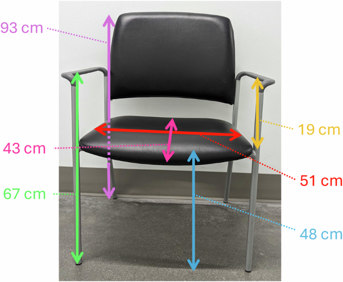
Chair used for experiment. Measurements are in centimeters, and approximate.
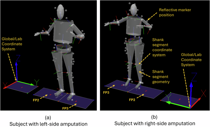
Visual 3D screenshots showing the Global/Lab coordinate system for subjects with left-side and right-side amputation, the reflective marker positions, the segment geometries, and the segment coordinate systems located on the proximal endpoint of each segment. (a) A subject with a left-sided amputation, with their right foot on FP2 and their left foot on FP3. The subject faces in the + X direction. (b) A subject with a right-sided amputation, with their right foot on FP3 and their left foot on FP2. The subject faces in the -X direction.
We asked subjects to stand up and sit down and recorded between 8 and 10 repetitions of stand-up and sit-down. We recorded all of the repetitions in a single trial. We cued subjects for each movement (“Stand up”, “Sit down”) and asked them to pause after standing up and to pause after sitting down. In the pauses between movements, we corrected their foot position if necessary. We asked the subjects to stand up and sit down without using their hands if possible. Eight of the nine subjects were able to stand up without hands. Five of the nine subjects were able to sit down without hands, and two were able to sit down without hands during some repetitions. Each subject’s hand use is detailed in Table 1.
Processing: Vicon Nexus
We used Vicon Nexus 2 (Vicon Motion Systems Ltd; Oxford, UK) to reconstruct, label, and fill the 3D marker data and to calculate the positions of the functional hip joint centers and functional knee axes. This section will describe the processing steps performed on each trial: the Static, Functional/ROM, and Dynamic (Sit-to-stand). See Included Files: Vicon for the files included for your use. All of the models and pipelines are included in the dataset, as well as the actual data files for each subject.
Processing the static trial
First, we opened the Static trial ([YYYYMMDD]_[SubjectCode]_static) in Vicon Nexus and attached the model “Full_Body_BELab_STS_DB.vst”. We ran the pipeline “Reconstruct.Pipeline”. We found a frame where all of the markers were visible, labeled the markers manually, and then cropped the trial to a few frames containing the selected frame. We ran the pipeline “Static.Pipeline”.
Later, after processing the Functional/ROM trial, we re-opened the Static trial and ran the pipeline “LE_Process_SCORE_SARA.Pipeline” to apply the functional hip joint centers and functional knee axes.
Processing the functional/ROM trial
First, we opened the Functional/ROM trial ([YYYYMMD]_[SubjectCode]_ROM) in Vicon Nexus. We ran the pipeline “Reconstruct_Label.Pipeline” to reconstruct the marker data and automatically label the markers. We checked that the markers were labeled correctly during the entire trial by inspecting the 3D reconstruction of the markers and inspecting graphs of the x, y, and z components of each marker trajectory. We labeled any unlabeled markers. We unlabeled or re-labeled incorrect labels. We did not fill gaps. We ran the pipeline “Functional.Pipeline”. Next, we ran “LE_Calibrate_SCORE_SARA.Pipeline” to calculate the positions of the SCORE25 functional hip joint centers and SCORE and SARA26 functional joint axes for the knee axes.
First, “LE_Calibrate_SCORE_SARA.Pipeline” creates six “OCST Bones” (Optimum Common Shape Technique) – one for each segment of the lower limb. The OCST Bones and the markers used to create them are as follows: Pelvis (RASI, LASI, RPSI, LPSI, RILC, LILC), RightThigh (RTHI, RTHIA, RTHIP, RTHII), LeftThigh (LTHI, LTHIA, LTHIP, LTHII), RightTibia (RTIB, RTIBA, RTIBI, RTIBP), LeftTibia (LTIB, LTIBA, LTIBI, LTIBP). We modified the marker lists for three subjects by removing markers that were missing from large portions of the Functional/ROM trial and by adding other markers if needed. For TF03, the Pelvis was modified by removing the LILC, and the RightThigh was modified by removing RTHIP. For TF04, the LeftThigh was modified by removing LTHIP and LTHII and adding LKNE and LGTR, the LeftTibia was modified by removing LTIBA, and the RightTibia was modified by removing RTIB. For TF05, the RightThigh was modified by removing RTHII and RTHIP and adding RKNE.
Second, “LE_Calibrate_SCORE_SARA.Pipeline” creates six markers: Pelvis_LeftThigh_score, the left functional hip joint center, Pelvis_RightThigh_score, the right functional hip joint center, RightThigh_RightTibia_score, a marker at the center of the right knee joint, RightThigh_RightTibia_sara, a marker lateral to the right knee joint (used with RightThigh_RightTibia_score to define an axis of right knee rotation), LeftThigh_LeftTibia_score, a marker at the center of the left knee joint, and LeftThigh_LeftTibia_sara, a marker lateral to the left knee joint (used with LeftThigh_LeftTibia_score to define an axis of left knee rotation). Note that many of the functional joint centers are slightly asymmetric on right and left; above-knee amputees often hold one side of their pelvis higher than the other due to muscular changes at the residual hip and due to socket and prosthesis configuration.
Processing the dynamic (Sit-to-Stand) trial
First, we opened the Dynamic (sit-to-stand) trial ([YYYYMMDD]_[SubjectCode]_sts_01). We ran the pipeline “Reconstruct_Label_Fill.Pipeline” to reconstruct the marker data, automatically label the markers, and fill gaps using a Woltering filter for gaps of up to 5 frames and Rigid Body Fills for every segment to fill gaps of up to 50 frames. The Pelvis Rigid Body Fill module was not “checked” and not run, because we preferred to fill all pelvis marker gaps manually.
We checked that the markers were labeled correctly during the entire trial by inspecting the 3D reconstruction of the markers and inspecting graphs of the x, y, and z components of each marker trajectory. We re-labeled markers that were unlabeled or mislabeled. We filled gaps, choosing Rigid Body fill whenever possible or using Pattern fill. We selected Source Markers from the same segment as the marker with the gap. We were careful to avoid choosing Source Markers that had been filled during the same period. We visually inspected the quality of each fill. When necessary, we “undid” the fill and re-filled the gap using different Source Markers.
We cropped some trials to remove the signals at the start or end of the trial. Reasons for cropping included to remove periods of the trial when some markers are not visible, to remove periods of talking recorded before the movements, to remove bad movements at the start or end, and to remove the first sit-down when a subject began the trial standing instead of sitting. These trials were cropped in Vicon, saved, un-cropped to restore the original number of frames, and re-saved. As a result, the cropped periods have no trajectories, and the frames are still included in the export.
We manually added events to the sit-to-stand trials: a “Foot OFF” event before the initiation of each stand-up movement and a “Foot ON” event after the completion of the sit-down movement. These events were added to the General row of events. The events were used to help us visualize the results in Visual 3D and were not used for any processing in MATLAB.
Later, after processing the Functional/ROM trial, we re-opened the Dynamic (sit-to-stand) trial and ran the pipeline “LE_Process_SCORE_SARA.Pipeline” to apply the functional hip joint centers and functional knee axes.
Processing: Visual 3D
We used Visual 3D (Has-Motion, Ontario, Canada) to create a 3D kinetic and kinematic model of each subject, then to calculate kinematic and kinetic signals, and to export the signals to a text file. This section will first describe the model and then describe the processing steps performed in Visual 3D. See Included Files: Visual 3D for the files included for your use. All of the models and pipelines are included in the dataset, as well as the actual workspace file for each subject, “[YYYYMMDD]_[SubjectCode]_STS.cmz.”
Markers are 3D targets imported from Vicon, and their names will be italicized. Landmarks are 3D targets created in Visual 3D, and their names will be italicized and bolded. Subject Data/Metrics are values or calculations that result in values. “Distance” is a built-in command that finds the straight-line distance between two positions.
For items that are bilateral (ex. RThigh and LThigh), only the right-sided derivations are included, and you should infer that the same process is followed for the left side.
Visual 3D model
Model overview
We used a 15-segment kinetic and kinematic model: 1 head, 1 thorax/abdomen, 1 pelvis, 2 upper arms, 2 forearms, 2 hands, 2 thighs, 2 shanks, and 2 feet. In addition, two Virtual Foot segments are included to calculate the ankle angles, but they are not kinetic (they do not have inertia and cannot be assigned forces or torques). We did not apply any inverse kinematic (IK) constraints and modeled all of the segment joints as 6-degree-of-freedom joints.
Segment properties: mass, center of mass, coordinate system, and inertial properties
The mass of each segment is calculated as a fraction of the subject’s total mass, and we used Visual 3D’s default mass fractions27, which are derived from Dempster28. The segments are modeled as geometric shapes. The head and hands are modeled using ellipsoids, the trunk/abdomen and pelvis are modeled using cylinders, and the remaining segments are modeled using cones. We used Visual 3D’s default for the segment coordinate system, which matches the laboratory coordinate system: the A/P Axis is +Y, and the Distal to Proximal axis is +Z29. We used Visual 3D’s default calculation for the moment of inertia for each segment, which uses the segment’s mass, the proximal and distal radii, and the segment geometry30, as described in Hanavan31. Notably, we modified the prosthesis-side shank segment in order to more accurately reflect the mass and inertial properties of the prosthesis: we changed its segment geometry to “custom” to enable changing of the default values and then divided the mass by 3, and changed the center of mass position to be 25% of the shank length below the top of the shank (from the default position of 42.7549% of the shank length below the top of the shank).
Subject data/metrics
Subject Data/Metrics are a type of variable that contains a value or a calculation that results in a value. They are bolded. The variables in Subject Data/Metrics can be used in landmark definitions, segment definitions, and pipeline commands. The following Subject/Data Metrics are used to define Landmarks and Segments in this dataset:
Marker = 0.014 [m].
Marker_base = 0.002 [m].
SHOULDER_OFFSET = (−0.17*Distance(LSHO,RSHO))-(Marker_Base + (0.5*Marker)) [m].
Right_Hand_Thickness = 0.024 [m]. Left_Hand_ Thickness = 0.024 [m].
Height [m] is entered for each subject.
Weight [kg] is entered for each subject.
Landmark definitions
Landmarks are 3D targets created in Visual 3D. Each landmark that is used to define a segment is described in Table 5.
Several landmarks are created to define the lower limb segments. The VISUAL 3D composite pelvis creates two landmarks, Right_Hip (bilateral)32, which are only used in this study to calculate the thigh radii. To create the knee joint center, RKJC (bilateral), a landmark F_RKNEE_L (“functional right knee lateral”) is created using a Starting Point of RightThigh_RightTibia_sara, an Ending Point RightThigh_RightTibia_score, and Projecting From RKNE (the lateral knee marker placed during the experiment). Similarly, a landmark F_RKNEE_M (“functional right knee medial”) is created using a Starting Point of RightThigh_RightTibia_sara, an Ending Point RightThigh_RightTibia_score, and Projected From RKNEM (the medial knee marker placed during the experiment). Finally, the landmark RKJC (“right knee joint center”) is created 50% between F_RKNEE_L and F_RKNEE_M. The landmark RKJC is used as the Distal Landmark for the RThigh, and the Proximal Landmark for the RShank. The ankle joint center, RAJC (bilateral), is created 50% between the markers RANK and RANKM.
Six landmarks are created to define the head. Right_Mid_Head (bilateral) is a landmark 50% between the markers RFHD and RBHD. Right_Base_Head (bilateral) is a landmark created at the global X and Y position of Right_Mid_Head, and at the Z position of C7. Right_Top_Head (bilateral) is a landmark created at the global X and Y position of Right_Mid_Head, and at the Z position of 0.936*Height of the subject.
Several landmarks were created to define the trunk segment. SUP_PELVIS, the proximal landmark for the trunk, was created by projecting a landmark within the Pelvis coordinate system (which is centered in the Pelvis segment) by 100% of the Pelvis segment height. MID_CLC7, the distal landmark for the trunk, is a landmark 50% between the markers C7 and CLAV. MID_STT10 is created at the global X and Y position of MID_CLC7, and the Z position of STRN. THORAX_X is defined with Starting Point CLAV, Ending Point C7, Lateral Object (on a plane) MID_STT10, and offset by 0.1 meters in the A/P direction and by half of the distance between CLAV and C7 in the axial direction.
Several landmarks are created to define the upper limb segments. The shoulder joint center, R_Shoulder_Center (bilateral), is created by projecting axially in the global coordinate system from RSHO by the length (−0.17*Distance(LSHO,RSHO))-(Marker_Base + (0.5*Marker)). The elbow joint center, REJC (bilateral), is created 50% between the markers RELB and RELBM. The wrist joint center, RWJC (bilateral), is created 50% between the markers RWRA and RWRB. The distal hand landmark, Right_Distal_Hand (bilateral), is defined with Starting Point RFIN, Ending Point RWJC, Lateral Object (on a plane) RWRA, and offset in the A/P direction by the length Marker_ Base + 0.5*Marker + (0.5*Right_Hand_Thickness).
Several landmarks are created to define the Virtual Foot segment. We followed “Virtual Foot Method 3 – Projected landmarks” from the Visual 3D Foot Tutorial33. This method projects the RAJC, R5FT, and RHEE markers onto the floor plane. The resulting markers are named RAJC_Floor, R5FT_Floor, and RHEE_Floor.
Segment definitions
Each segment is primarily described in Table 6, which includes the inputs used to create the segment. Because the segment radii are defined using 3D marker positions, the model is scaled to the subject automatically.
We used virtual foot segments to define the ankle angles. The virtual foot enforces the assumption that the foot is parallel to the floor during neutral posture. We followed “Virtual Foot Method 3 – Projected landmarks” from the Visual 3D Foot Tutorial33. The virtual foot segment is tracked using the non-projected foot markers, and the ankle angle is computed between the virtual foot and the shank/calf segment.
One single-subject model modification was made – for subject TF07, RKNE and RGTR were added to the tracking markers of the Right Thigh segment to improve tracking. No other subjects required modifications.
Visual 3D processing
Workspace setup
We began by entering the following settings into each Visual 3D workspace. In the Settings menu, we checked “Use Processed Analogs for Ground Reaction Force Calculations”, “Use Processed Targets for Model/Segment/LinkModelBased items”, and “Use Biomechanics Conventions”. In the Force menu, we set “Distance of FP center of Force Pressure to nearest segment” to 0.2 m and “Minimum Force Platform Value” to 20 N.
We loaded the static trial into the workspace using Model > Hybrid Model from C3D File, followed by selecting the c3d file of the subject’s static trial, “[YYYYMMDD]_[SubjectCode]_static.c3d”. The model file was applied by clicking Model and then Apply Model Template, then selecting either “STS_DB_ProsthesisL.mdh” for subjects with left-side amputations or “STS_DB_ProsthesisR.mdh” for subjects with right-side amputations. The subject’s Height in meters and Weight in kg were entered into the Subject Data/Metrics. Build Model was clicked.
The dynamic trial was opened using File > Open/Add, selecting “Insert new files into your currently open workspace”, followed by selecting the c3d file of the subject’s dynamic (sit-to-stand) trial, “[YYYYMMDD]_[SubjectCode]_sts_01.c3d”, and Open.
The model was assigned to the dynamic trial using Model > Assign Model to Motion Files, checking the box next to the dynamic trial, and clicking OK.
Pipelines
Each of the following pipelines was opened and executed using the following options: clicked Pipeline > Open Pipeline… > Replace > Execute Pipeline.
The pipeline “01_Combine_FP.v3s” creates a combined force structure from the right and left foot force plates, with combined forces, center of pressures, and moments. The combined force structure is named FS1.
The pipeline “02_Kinetics_Kinematics.v3s” low pass filters the marker trajectories at 6.0 Hz using a bidirectional Butterworth filter, and low pass filters the force plate signals at 15 Hz using a bidirectional Butterworth filter. Next, it uses Compute_Model_Based_Data to compute kinematics and kinetics (joint torque and joint power) for the lower limb joints (ankle, knee, hip). For left-side angles and torques of joints, we negated Y and Z so that right and left-side joint torques have corresponding positive and negative directions. The ground reaction forces (GRF), joint torques, and joint powers are normalized by dividing by the subject Mass in kg. Joint torque was computed using the joint_moment function, choosing the joint of interest as “joint” and choosing the proximal segment as “resolution coordinate system”. Joint power was computed using joint_power_scalar function. Joint power is not a vector, so it does not have an X, Y, or Z component. The pipeline also calculates R_GRF and L_GRF (ground reaction forces), R_COP and L_COP (center of pressure), and COM (center of mass). When a force plate’s force reads less than the Minimum Force Platform Value (20 N), the R_GRF and L_GRF are equal to zero, and the R_COP and L_COP are NaN. Finally, the pipeline uses Compute_Model_Based_Data to find the proximal and distal segment positions for all segments within the lab/global coordinate system (see Fig. 3).
The pipeline “03_Copy_Anthropometrics.v3s” uses Evaluate_Expression to copy anthropometric values for each subject to the “GLOBAL” workspace so they can be exported using the next pipeline. For each segment, the following properties are included: origin, length, proximal radius, and distal radius.
The pipeline “04_Export.v3s” asks the user to select the folder where the text files will be saved. Then, this pipeline exports all of the txt files, which are described in Visual 3D: exported txt files, to the selected folder.
Processing: MATLAB
We used MATLAB R2022B to perform all further data processing. Mat files are created at each step of processing: Raw, Secondary variables, Filtered, and Segmented.
Each subject has a script named “[SubjectCode]_processing.m”, and the sections below labeled “Step 0”, “Step 1” etc, correspond directly to sections in the processing script with the same names. See Included Files: MATLAB for the files included for your use. All of the subject-specific files and all of the functions used for processing are included in the dataset.
MATLAB variables and field names will be bolded in this section.
MATLAB Step 0 – Initialize and create subject info file
First, we initialize subject-specific parameters by creating a variable, subject, which includes the subject’s height, weight, prosthesis side, intact side, the date of collection, their Subject Code, the subject’s folder name, and a dictionary to assign muscles with the corresponding EMG sensor number.
We also include variables indicating the number of repetitions for the up, down, and full movements for this subject and indicating the index values of “bad” reps, including reps with bad movement (rep will be deleted), reps with hand use (the rep’s kinetic variables will be set to NaN), and reps indicating the index values of any artifacts in the EMG for each muscle (the muscle’s EMG signal for that rep will be set to NaN).
We also include a variable to indicate how much we want to “zoom out” from the initial segmentation of each repetition. We define the variable zoom_out, a vector of positive numbers, and each entry in zoom_out will result in a separate copy of the final, segmented data structure. The units of zoom_out are the percent of the length of the segmented repetition. For example, zoom_out = [0, 5] will save a copy of the un-zoomed dataset showing 0% to 100% and a copy of the dataset that is “zoomed out” to show from −5% to 105% of the movement. See section Segmentation: Intact vs. Prosthesis segmentation and “zooming out” for details.
All subject parameters are stored in a parameter structure variable named subject. The structure is saved as “[SubjectCode]_subjectinfo.mat”.
MATLAB Step 1 – raw
Next, we loaded the text file “[Date_SubjectCode]_sts_01.c3d.txt” using the function “v3d_import.m”, a function created using sample code provided by Visual 3D34. We saved the signals into a structure array in the MATLAB workspace. The structure array is named data_raw and has fields “prosthesis_side”, containing the prosthesis-side signals, “intact_side”, containing the intact-side signals, “M”, containing the “medial” signals like center of mass, “EMG_raw”, containing the raw EMG signals. Within each field will be variable names, for example, “knee_angle_X”, each of which contains a vector of the signal. The structure data_raw also has two variables, time and time_EMG. We saved the structure data_raw as “[SubjectCode]_01_raw/[SubjectCode]_STS_01_raw.mat”.
MATLAB Step 2 – Secondary variables
We loaded the file “[SubjectCode]_STS_01_raw.mat” and renamed the structure data. For only subject TF01, we fix a delay in the EMG signals by cropping 1807 frames from the beginning of each EMG signal and padding 1807 frames of zeros to the end of each EMG signal.
Next, we addressed NaN values. Most variables have some NaNs at the beginning or end of the trial, and the variables data.prosthesis_side.COP_X, Y, and Z, data.intact_side.COP_X, Y, and Z, and data.M.COP_combined_X, Y, and Z have additional NaN periods during the middle of most trials because in Visual 3D COPs were set equal to NaN when the corresponding GRF forces dropped below a threshold. NaNs introduce a problem to our data processing because they prevent a signal from being filtered or interpolated. To address this problem, we searched for NaNs in each variable. Whenever possible, we replaced each period of NaNs with the previous value of the signal. If a period of NaNs was at the start of the signal, we replaced it with the next non-NaN value.
We also down-sampled the variables COP_combined_X, Y, and Z from 2000 Hz to 200 Hz sampling rate to match the sampling rate of the other signals (except signals in EMG_raw, which are kept at 2000 Hz).
We also performed numerical differentiation. Before differentiating, we filtered the input position/velocity signals with a 4th-order bidirectional Butterworth filter at 5 Hz because differentiation amplifies noise. We calculated joint angular velocity and angular acceleration in X and calculated the linear velocity and linear acceleration of the COPs and COMs in X, Y, and Z.
We copied the data structure to a variable data_secondary and saved it as “[SubjectCode]_02_secondary/[SubjectCode]_STS_01_secondary.mat”.
MATLAB Step 3 – filter
We low-pass-filtered all of the non-EMG variables in the data_secondary structure using a 4th-order, bidirectional Butterworth filter at 8 Hz, and the resultant structure is saved as data_filtered.
Next, we created the EMG envelopes by band-pass filtering the raw EMG signal between 20 and 450 Hz, rectifying the signal, and low-pass-filtering the signal using a 4th-order bidirectional Butterworth filter at 3 Hz. We also down-sampled the envelopes to 200 Hz to match the remaining non-EMG signals. We saved the envelopes to a new field, data_filtered.EMG. The branch data_filtered.EMG_raw is not modified – the raw EMG signals are unfiltered and still sampled at 2000 Hz. To plot raw EMG, use data_filtered.EMG_raw.time_EMG_raw.
We saved the resulting data_filtered structure as “[SubjectCode]_03_filtered/[SubjectCode]_STS_01_filtered.mat”.
MATLAB Step 4 – Find start and stop indices
We found the index (frame) values of the start and stop of each stand-up and sit-down using threshold values relating to the knee angle, knee velocity, and the duration of movement. The index values are found using the prosthesis-side knee and the intact-side knee separately. The intact knee and prosthesis knee are not perfectly synchronized, and the intact knee usually starts and ends the movement earlier than the prosthesis knee. Both presentations of the data can be insightful.
We loaded the file “[SubjectCode]_STS_01_filtered.mat” and renamed the structure data. We found the start and stop indices based on four thresholds to find stand-up and four thresholds to find sit-down. The intact and prosthesis sides often required different threshold values, and the thresholds were adjusted by hand based on our experience. The thresholds are used in both segment_up and segment_down functions and often had different values for each. pos_ths_sitting is a threshold on the knee_position_X of the intact or prosthesis-side. pos_ths_sitting has units of degrees, a default value of −90, and a range of −90 to −60. For stand-up and sit-down, it should be less negative than the minima of the knee position. pos_ths_standing is a threshold on the knee_position_X of the intact or prosthesis-side. pos_ths_standing has units of degrees, a default value of −15, and a range of −20 to 5. For stand-up and sit-down, it should be more negative than the maxima of the knee position. vel_ths is a threshold on the knee_vel_X and has units of degrees per second. For stand-up, vel_ths’s default value is 5, and the range is 5 to 15. For sit-down, vel_ths’s default value is −5, and the range is −10 to −5. too_close is used to eliminate events that are too close together in time. It is the required number of frames (at 200 Hz) between events of the same type. The units are frames.
Stand-Up: start and stop indices
The start and stop events for the stand-up movement are detected using a multi-step process by the function “segment_up.m”. For stand-up, an excess of possible start and stop events are detected using:
>stand_start = find([0; diff(knee_vel_X > vel_ths)]==1 & (knee_angle_X < pos_ths_sitting));
> stand_stop = find([0; diff(knee_vel_ < vel_ths)]==1 & (knee_angle_X > pos_ths_standing));
The variables stand_start and stand_stop will be vectors containing index values of possible events. The two vectors are unlikely to have the same number of events, initially. A series of loops are used to remove events of the same name that are too close together, to remove events that are out of order, and to remove duplicate events. The result is an ordered list of start and stop index values, with one start and one stop per stand-up repetition.
Sit-Down: start and stop indices
The start and stop events for the stand-up movement are detected using a multi-step process by the function “segment_up.m”. For stand-up, an excess of possible start and stop events are detected using:
>sit_start = find([0; diff(knee_vel_X < vel_ths)]==1 & (knee_angle_X > pos_ths_sitting));
> sit_stop = find([0; diff(knee_vel_X > vel_ths)]==1 & (knee_angle_X < pos_ths_standing));
The variables sit_start and sit_stop will be vectors containing index values of possible events. The two vectors are unlikely to have the same number of events, initially. A series of loops are used to remove events of the same name are too close together, to remove events that are out of order, and to remove duplicate events. The result is an ordered list of start and stop index values, with one start and one stop per sit-down repetition.
Full movement: combining stand-up and sit-down indices
The function “segment_s2s.m” combines the index values of stand-up and sit-down to create index values for the start and stop of the full movement: stand-up-sit-down. The function checks that the first movement is “up”, and that each “up” is paired with a “down”. The function deletes any mis-ordered events.
Finally, the start and stop index values for “up” “down” and “full” are organized in a structure and saved into the folder “[SubjectCode]_04_start_stop_index/ [SubjectCode]_index_intact_segmentation_zoom00.mat, [SubjectCode]_index_prosthesis_segmentation_zoom00.mat”.
MATLAB Step 5: segment
Next, we segment the trial in several ways: based on the prosthesis-side segmentation and the intact-side segmentation, and for each entry in “zoom out”. Figure 4 and Figure 5 demonstrate the differences between the different types of segmentations. We also create new variables to improve usability, we handle “bad” repetitions, and then we save a separate copy of the dataset for each of the segmentation types.
We perform a prosthesis-side and intact-side segmentation of the dataset for each entry in subject.zoom_out, a variable defined in MATLAB Step 0 – Initialize and Create Subject Info File. See the section Segmentation: Intact vs. Prosthesis segmentation and “zooming out”. At this step, we also completely remove “bad movements” by removing the column(s) from every variable.
We segmented and interpolated the signals for each repetition to the same number of frames (1001 frames, or 1001*10 frames for EMG_raw) regardless of the zoom percent. We also create variables data.stopwatch and data.percent_completion, and data.EMG_raw.stopwatch_EMG_raw and data.EMG_raw.percent_completion_EMG_raw.
We also add variables to document the segmentation type that has been opened. We save new variables into data.segmentation_info.segmentation_type, a string equaling either ‘prosthesis_side’ or ‘intact_side’ We also save data.segmentation_info.index_zoomed.up, .down, and .full, 2 × n vectors of the start (row 1) and stop (row 2) indices, referring to the zoomed index values used to segment the filtered data for the segmentation. We add two variables each to data.up, data.down, and data.full. The first is index_0_percent, the index value (in each column of segmented data) of the rep’s original “start”. This is the index where percent_completion ≈ 0 and where stopwatch = 0. The second is .index_100_percent, the index value where percent_completion ≈ 100. Similarly, we add two variables each to data.up.EMG_raw, data.down.EMG_raw, and data.full.EMG_raw. The first is .index_0_percent_EMG_raw, the index value (in each column of segmented data) of the rep’s original “start”. This is the index where percent_completion_EMG_raw ≈ 0 and where stopwatch_EMG_raw = 0. The second is .index_100_percent_EMG_raw, the index value where percent_completion_EMG_raw ≈ 100.
Next, we replace the signal with NaN during “bad” reps. During reps when the subject used hands, we replace the following types of signals: torques, powers, and COPs. During the reps when there are EMG artifacts, we replace the EMG and EMG_raw signals of the muscle with the artifact.
Finally, we save the segmented data files. As published, we create the following segmented files for every subject:
“[SubjectCode]_STS_01_intact_seg_zoom00.mat”
“[SubjectCode]_STS_01_intact_seg_zoom10.mat”
“[SubjectCode]_STS_01_intact_seg_zoom20.mat”
“[SubjectCode]_STS_01_intact_seg_zoom30.mat”
“[SubjectCode]_STS_01_prosthesis_seg_zoom00.mat”
“[SubjectCode]_STS_01_prosthesis_seg_zoom10.mat”
“[SubjectCode]_STS_01_prosthesis_seg_zoom20.mat”
“[SubjectCode]_STS_01_prosthesis_seg_zoom30.mat”
“intact_seg” indicates that the file was segmented using the intact-side knee position and velocity, whereas “prosthesis_seg” indicates that the file was segmented using the prosthesis-side knee position and velocity. “zoom00” means the original segmented indices are used. “zoom10” means the data has been zoomed out 10% from the original segmented indices, adding 5% on each side. “zoom20” means the data has been zoomed out 20% from the original segmented indices, adding 10% on each side. “zoom30” means the data has been zoomed out 30% from the original segmented indices, adding 15% on each side.
We also created and saved a series of result figures for each subject using “plot_after_segmentation.m”. As published, 60 figures are created, representing all combinations of the following options: (2 zoom-out options: 0% and 30%) * (2 segmentation types: intact segmentation, prosthesis segmentation) * (3 parts: up, down, full) * (5 “sides”: intact-side, prosthesis-side, M, EMG, and EMG raw). Every variable in each side is added to a subplot. Some subjects have empty plots or sparse plots. This is not an error; it is likely due to repetitions being removed due to EMG problems or using hands. The figures are saved for each subject inside “[SubjectCode]_06_segmentation_figures”.
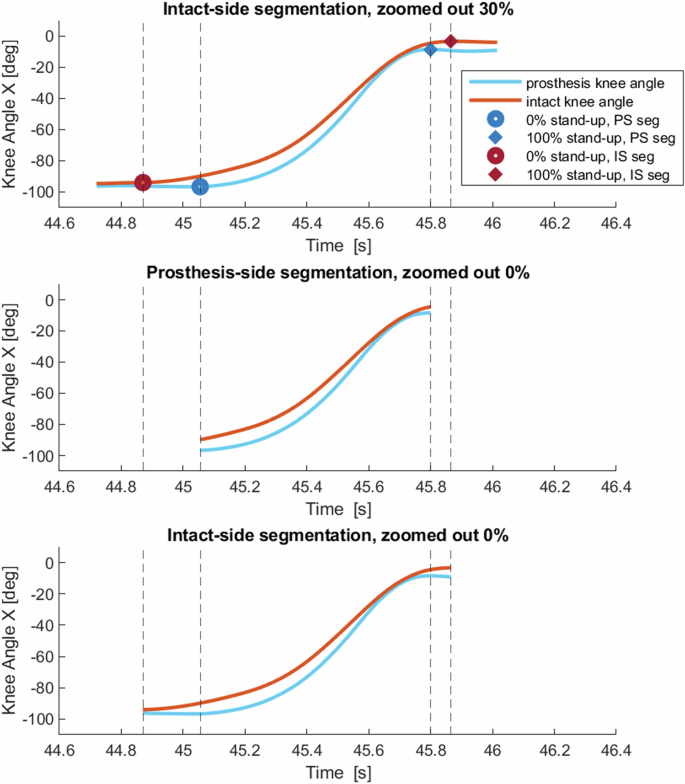
Figure demonstrating the difference between intact-side and prosthesis-side segmentations. The red line is the intact knee angle, and the blue line is the prosthesis knee angle from the same repetition. Top: intact-side segmentation, zoomed out by 30%, with markers and vertical lines indicating the start and stop of the 0% prosthesis-side segmentation and 0% intact-side segmentation. Middle: 0% zoomed prosthesis-side segmentation. Bottom: 0% zoomed intact-side segmentation.
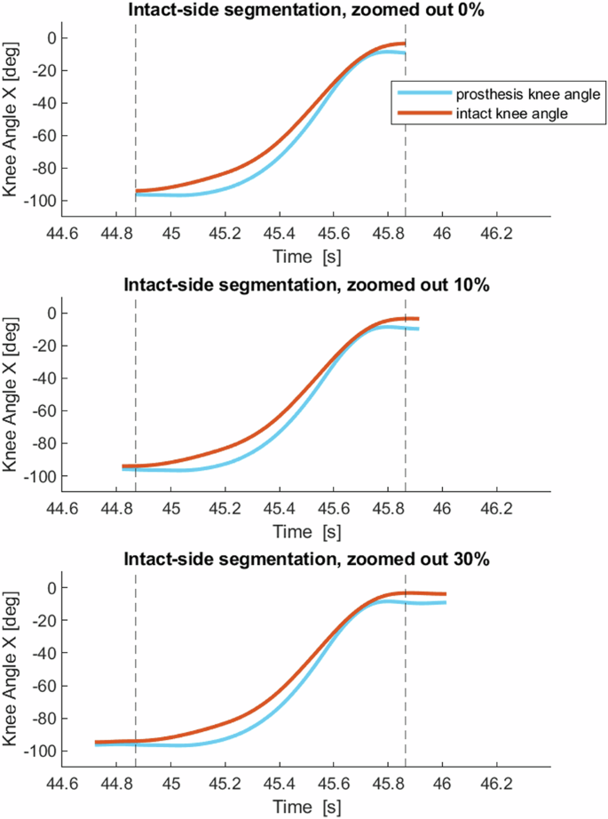
Figure demonstrating three zoom options for one repetition of stand-up with intact-side segmentation. The red line is the intact knee angle. The blue line is the prosthesis knee angle. The vertical lines show the start and stop of 0% zoom. Top: 0% zoomed out. Middle: 10% zoomed out. Bottom: 30% zoomed out. On the x-axis is time in seconds.
MATLAB Step 6: export to csv
Finally, we export the segmented data to csv files for non-MATLAB-users. Every segmented trial is saved into two different csv files: one containing all of the signals except EMG_raw, and one containing only EMG_raw. This is done for simplicity because EMG_raw is sampled at 10x the frame rate of the other signals.
Every entry in the MATLAB structure is saved into the spreadsheet by the function ‘export_csv.m’.
The csv files are organized based on the MATLAB structure. Row 1 indicates field 1, Row 2 indicates field 2, Row 3 indicates field 3, Row 4 indicates the name of the variable, and Row 5 indicates the column number (indexing starts with 1). Row 6 is the first frame of the signal. Some of the header rows will be empty for some variables – for example, “data.up.prosthesis_side.knee_torque” will be written as Row 1: ‘up’, Row 2: ‘prosthesis_side’, Row 3: ‘‘, Row 4: ‘knee_torque’, For variables with multiple columns (most variables), each repetition will be written to a separate column of the spreadsheet, and Row 5 will indicate the column number.
Data Records
The dataset is available at FigShare, reference number 26282872, with this section being the primary source of information on the availability and content of the data being described20.
Folders were zipped before uploading to Figshare.
The zipped folders are: ViconDB_STS, V3D_STS, each folder within MATLAB_DB, and each subject’s segmentation_figures folder (MATLAB_DB/ [Date_SubjectCode]/ [SubjectCode]_06_segmentation_figures). The files and sub-folders of zipped and unzipped folders are listed below. Zipped folders are indicated by “(ZIPPED)”.
Included files: vicon nexus
DB_TF_STS/ViconDB_STS.zip (ZIPPED)
Vicon: workspace/data files
DB_TF_STS/ViconDB_STS/[Date_SubjectCode]/[Date_SubjectCode]/
[Date_[SubjectCode].Session.enf
[Date_[SubjectCode]_ROM.Trial.enf
[Date_[SubjectCode]_ROM.c3d
[Date_[SubjectCode]_ROM.digitaldevices.xml
[Date_[SubjectCode]_ROM.history
[Date_[SubjectCode]_ROM.system
[Date_[SubjectCode]_ROM.x1d
[Date_[SubjectCode]_ROM.x2d
[Date_[SubjectCode]_ROM.xcp
[Date_[SubjectCode]_passive.mp
[Date_[SubjectCode]_passive.vsk
[Date_[SubjectCode]_static.Trial.enf
[Date_[SubjectCode]_static.c3d
[Date_[SubjectCode]_static.digitaldevices.xml
[Date_[SubjectCode]_static.history
[Date_[SubjectCode]_static.system
[Date_[SubjectCode]_static.x1d
[Date_[SubjectCode]_static.x2d
[Date_[SubjectCode]_static.xcp
[Date_[SubjectCode]_sts_01.Trial.enf
[Date_[SubjectCode]_sts_01.c3d
[Date_[SubjectCode]_sts_01.digitaldevices.xml
[Date_[SubjectCode]_sts_01.history
[Date_[SubjectCode]_sts_01.system
[Date_[SubjectCode]_sts_01.x1d
[Date_[SubjectCode]_sts_01.x2d
[Date_[SubjectCode]_sts_01.xcp
LatestCalibration [YYYYMMDDHHMMSS].x2d.sup
Vicon: model files
DB_TF_STS/ViconDB_STS/Vicon_Model_Files/
Full_Body_BELab_STS_DB.vst
Full_Body_BELab_STS_DB.mkr
Vicon: pipeline files
DB_TF_STS/ViconDB_STS/Vicon_Pipeline_Files/
Reconstruct.Pipeline
Static.Pipeline
Reconstruct_label.Pipeline
Functional.Pipeline
Reconstruct_Label_Fill.Pipeline
LE_Calibrate_SCORE_SARA.Pipeline
LE_Process_SCORE_SARA.Pipeline
Included files: Visual 3D
DB_TF_STS/V3D_STS.zip (ZIPPED)
Visual 3D: workspace/data files
DB_TF_STS/V3D_STS/
[YYYYMMDD]_[SubjectCode]_STS.cmz
Each subject has a single workspace file which contains the subject model, processed dynamic trial, and all signals. It requires the program Visual3D to open it.
Visual 3D: model files
DB_TF_STS/V3D_STS/VISUAL 3D_Model_Files
STS_DB_ProsthesisL.mdh
STS_DB_ProsthesisR.mdh
Visual 3D: pipeline files
DB_TF_STS/V3D_STS/VISUAL 3D_Pipeline_Files
01_Combine_FP.v3s
02_Kinetics_Kinematics.v3s
03_Copy_Anthropometrics.v3s
04_Export_STS.v3s
You can open these pipelines in Visual 3D to see the commands and options, as either text or with a GUI. You can also open the pipeline functions using text editors. We recommend Notepad++. Follow the directions here35 to install an (optional) user-defined language package that will apply a color scheme and formatting to the text.
Visual 3D: exported txt files
DB_TF_STS/MATLAB_STS/[SubjectCode]_MATLAB/[SubjectCode]_01_raw/
“[Date_SubjectCode]_sts_01.c3d.txt” includes lower-limb joint variables, R and L GRF, EMGs, COM, R and L COP, and a combined COP named FS1_1. The COM and COPs are measured in meters and are defined relative to the Global/Lab coordinate system (see Fig. 3). All three components (X, Y, and Z) are included for some signals. The file includes one row for each frame. GRFs, torques, and powers were normalized by dividing by the subject’s mass in kg. Row 2 includes the variable name (ex. ‘R_knee_angle’). Row 5 specifies the X, Y, or Z component.
The spreadsheet includes variables with two frame rates, 200 Hz and 2000 Hz. The frame rate is 200 Hz for columns 1–94. These columns contain signal in approximately the first 10% of the rows, followed by NaN in the remaining 90% of the rows. The frame rate is 2000 Hz for variables in columns 95–113. These columns contain signals for approximately 100% of the rows.
The EMG signals are in columns 101–110, labeled “Sensor1.IM EMG1” through “Sensor16.IM EMG16”. Each subject wore 4 EMG sensors at a time, so only 4 of these 16 columns will contain information. The four sensors used for each subject and their corresponding muscles are indicated in Table 1. The 12 columns representing unused electrodes will equal 0 in every row.
This text file is the only text file which we imported into MATLAB.
“[Date_SubjectCode]_sts_01.c3d_segment_positions.txt” includes the proximal and distal locations of each segment. The positions are measured in meters and are defined relative to the Global/Lab coordinate system (see Fig. 3). All three components (X, Y, and Z) are included. The file includes one row for each frame. The frame rate is 200 Hz.
“[Date_SubjectCode]_sts_01.c3d_target_raw.txt” includes the raw positions of every reflective marker. The names correspond to the Vicon model. The positions are measured in meters and are defined relative to the Global/Lab coordinate system (see Fig. 3). All three components (X, Y, and Z) are included. The file includes one row for each frame. The frame rate is 200 Hz.
“[Date_SubjectCode]_sts_01.c3d_target_filtered.txt” includes the filtered positions of every reflective marker. The names correspond to the Vicon model. The positions are measured in meters and are defined relative to the Global/Lab coordinate system (see Fig. 3). All three components (X, Y, and Z) are included. The file includes one row for each frame. The frame rate is 200 Hz.
“[Date_SubjectCode]_sts_01.c3d_anthropometrics.txt” includes the anthropometric measures of the subject model. For every segment, the distal radius, length, origin, and proximal radius are included. These measures are derived from the static trial. Each anthropometric variable has one value in meters.
“[Date_SubjectCode]_sts_01.c3d_analog_raw.txt” includes the raw signals from force plates (FP) 2 and 3. The file includes one row for each frame. The frame rate is 2000 Hz. The naming convention follows:
Force.Fx2 is the X force from FP2
Force.Fy2 is the Y force from FP2
Force.Fz2 is the Z force from FP2
Force.Fx3 is the X force from FP3
…
Moment.Mz3 is the Z moment (torque) from FP3
“[Date_SubjectCode]_sts_01.c3d_analog_filtered.txt” includes the filtered signals from force plates (FP) 2 and 3. The naming convention matches _analog_raw.txt. The file includes one row for each frame. The frame rate is 2000 Hz.
“[Date_SubjectCode]_sts_01.c3d_force_cofp_freemoment.txt” includes the filtered force, cofp, and freemoment signals for FP2, FP3, and FS1_1 (a combined force structure representing FP2 and FP3). Visual 3D does not calculate raw versions explicitly due to the settings used (see Visual 3D Settings). All three components (X, Y, and Z) are included. The file includes one row for each frame. The frame rate is 2000 Hz.
Included Files: MATLAB
MATLAB: workspace/data files
Each subject has a folder containing folders and files, DB_TF_STS/MATLAB_STS/[SubjectCode]_MATLAB (ZIPPED). The contents follow.
[SubjectCode]_processing.m
[SubjectCode]_subjectinfo.mat
[SubjectCode]_01_raw/
[YYYYMMDD]_[SubjectCode]_sts_01.c3d.txt
[YYYYMMDD]_[SubjectCode]_sts_01.c3d_analog_filtered.txt
[YYYYMMDD]_[SubjectCode]_sts_01.c3d_analog_raw.txt
[YYYYMMDD]_[SubjectCode]_sts_01.c3d_anthropometrics.txt
[YYYYMMDD]_[SubjectCode]_sts_01.c3d_force_cofp_freemoment.txt
[YYYYMMDD]_[SubjectCode]_sts_01.c3d_segment_positions.txt
[YYYYMMDD]_[SubjectCode]_sts_01.c3d_target_filtered.txt
[YYYYMMDD]_[SubjectCode]_sts_01.c3d_target_raw.txt
[SubjectCode]_STS_01_raw.mat
[SubjectCode]_02_secondary/
[SubjectCode]_STS_01_secondary.mat
[SubjectCode]_03_filtered/
[SubjectCode]_STS_01_filtered.mat
[SubjectCode]_04_start_stop_index/
[SubjectCode]_index_intact_segmentation_zoom00.fig
[SubjectCode]_index_intact_segmentation_zoom00.mat
[SubjectCode]_index_prosthesis_segmentation_zoom00.fig
[SubjectCode]_index_prosthesis_segmentation_zoom00.mat
[SubjectCode]_05_segmented/
[SubjectCode]_STS_01_intact_seg_zoom00.mat
[SubjectCode]_STS_01_intact_seg_zoom10.mat
[SubjectCode]_STS_01_intact_seg_zoom20.mat
[SubjectCode]_STS_01_intact_seg_zoom30.mat
[SubjectCode]_STS_01_prosthesis_seg_zoom00.mat
[SubjectCode]_STS_01_prosthesis_seg_zoom10.mat
[SubjectCode]_STS_01_prosthesis_seg_zoom20.mat
[SubjectCode]_STS_01_prosthesis_seg_zoom30.mat
[SubjectCode]_06_segmentation_figures/ (ZIPPED)
[SubjectCode]_STS_01_intact_side_seg_zoom00_down_EMG.fig
[SubjectCode]_STS_01_intact_side_seg_zoom00_down_EMG_raw.fig
[SubjectCode]_STS_01_intact_side_seg_zoom00_down_M.fig
[SubjectCode]_STS_01_intact_side_seg_zoom00_down_intact_side.fig
[SubjectCode]_STS_01_intact_side_seg_zoom00_down_prosthesis_side.fig
[SubjectCode]_STS_01_intact_side_seg_zoom00_full_EMG.fig
[SubjectCode]_STS_01_intact_side_seg_zoom00_full_EMG_raw.fig
[SubjectCode]_STS_01_intact_side_seg_zoom00_full_M.fig
[SubjectCode]_STS_01_intact_side_seg_zoom00_full_intact_side.fig
[SubjectCode]_STS_01_intact_side_seg_zoom00_full_prosthesis_side.fig
[SubjectCode]_STS_01_intact_side_seg_zoom00_up_EMG.fig
[SubjectCode]_STS_01_intact_side_seg_zoom00_up_EMG_raw.fig
[SubjectCode]_STS_01_intact_side_seg_zoom00_up_M.fig
[SubjectCode]_STS_01_intact_side_seg_zoom00_up_intact_side.fig
[SubjectCode]_STS_01_intact_side_seg_zoom00_up_prosthesis_side.fig
[SubjectCode]_STS_01_intact_side_seg_zoom30_down_EMG.fig
[SubjectCode]_STS_01_intact_side_seg_zoom30_down_EMG_raw.fig
[SubjectCode]_STS_01_intact_side_seg_zoom30_down_M.fig
[SubjectCode]_STS_01_intact_side_seg_zoom30_down_intact_side.fig
[SubjectCode]_STS_01_intact_side_seg_zoom30_down_prosthesis_side.fig
[SubjectCode]_STS_01_intact_side_seg_zoom30_full_EMG.fig
[SubjectCode]_STS_01_intact_side_seg_zoom30_full_EMG_raw.fig
[SubjectCode]_STS_01_intact_side_seg_zoom30_full_M.fig
[SubjectCode]_STS_01_intact_side_seg_zoom30_full_intact_side.fig
[SubjectCode]_STS_01_intact_side_seg_zoom30_full_prosthesis_side.fig
[SubjectCode]_STS_01_intact_side_seg_zoom30_up_EMG.fig
[SubjectCode]_STS_01_intact_side_seg_zoom30_up_EMG_raw.fig
[SubjectCode]_STS_01_intact_side_seg_zoom30_up_M.fig
[SubjectCode]_STS_01_intact_side_seg_zoom30_up_intact_side.fig
[SubjectCode]_STS_01_intact_side_seg_zoom30_up_prosthesis_side.fig
[SubjectCode]_STS_01_prosthesis_side_seg_zoom00_down_EMG.fig
[SubjectCode]_STS_01_prosthesis_side_seg_zoom00_down_EMG_raw.fig
[SubjectCode]_STS_01_prosthesis_side_seg_zoom00_down_M.fig
[SubjectCode]_STS_01_prosthesis_side_seg_zoom00_down_intact_side.fig
[SubjectCode]_STS_01_prosthesis_side_seg_zoom00_down_prosthesis_side.fig
[SubjectCode]_STS_01_prosthesis_side_seg_zoom00_full_EMG.fig
[SubjectCode]_STS_01_prosthesis_side_seg_zoom00_full_EMG_raw.fig
[SubjectCode]_STS_01_prosthesis_side_seg_zoom00_full_M.fig
[SubjectCode]_STS_01_prosthesis_side_seg_zoom00_full_intact_side.fig
[SubjectCode]_STS_01_prosthesis_side_seg_zoom00_full_prosthesis_side.fig
[SubjectCode]_STS_01_prosthesis_side_seg_zoom00_up_EMG.fig
[SubjectCode]_STS_01_prosthesis_side_seg_zoom00_up_EMG_raw.fig
[SubjectCode]_STS_01_prosthesis_side_seg_zoom00_up_M.fig
[SubjectCode]_STS_01_prosthesis_side_seg_zoom00_up_intact_side.fig
[SubjectCode]_STS_01_prosthesis_side_seg_zoom00_up_prosthesis_side.fig
[SubjectCode]_STS_01_prosthesis_side_seg_zoom30_down_EMG.fig
[SubjectCode]_STS_01_prosthesis_side_seg_zoom30_down_EMG_raw.fig
[SubjectCode]_STS_01_prosthesis_side_seg_zoom30_down_M.fig
[SubjectCode]_STS_01_prosthesis_side_seg_zoom30_down_intact_side.fig
[SubjectCode]_STS_01_prosthesis_side_seg_zoom30_down_prosthesis_side.fig
[SubjectCode]_STS_01_prosthesis_side_seg_zoom30_full_EMG.fig
[SubjectCode]_STS_01_prosthesis_side_seg_zoom30_full_EMG_raw.fig
[SubjectCode]_STS_01_prosthesis_side_seg_zoom30_full_M.fig
[SubjectCode]_STS_01_prosthesis_side_seg_zoom30_full_intact_side.fig
[SubjectCode]_STS_01_prosthesis_side_seg_zoom30_full_prosthesis_side.fig
[SubjectCode]_STS_01_prosthesis_side_seg_zoom30_up_EMG.fig
[SubjectCode]_STS_01_prosthesis_side_seg_zoom30_up_EMG_raw.fig
[SubjectCode]_STS_01_prosthesis_side_seg_zoom30_up_M.fig
[SubjectCode]_STS_01_prosthesis_side_seg_zoom30_up_intact_side.fig
[SubjectCode]_STS_01_prosthesis_side_seg_zoom30_up_prosthesis_side.fig
[SubjectCode]_07_segmented_csv_files/
[SubjectCode]_STS_01_intact_seg_zoom00.csv
[SubjectCode]_STS_01_intact_seg_zoom00_EMG_raw.csv
[SubjectCode]_STS_01_intact_seg_zoom10.csv
[SubjectCode]_STS_01_intact_seg_zoom10_EMG_raw.csv
[SubjectCode]_STS_01_intact_seg_zoom20.csv
[SubjectCode]_STS_01_intact_seg_zoom20_EMG_raw.csv
[SubjectCode]_STS_01_intact_seg_zoom30.csv
[SubjectCode]_STS_01_intact_seg_zoom30_EMG_raw.csv
[SubjectCode]_STS_01_prosthesis_seg_zoom00.csv
[SubjectCode]_STS_01_prosthesis_seg_zoom00_EMG_raw.csv
[SubjectCode]_STS_01_prosthesis_seg_zoom10.csv
[SubjectCode]_STS_01_prosthesis_seg_zoom10_EMG_raw.csv
[SubjectCode]_STS_01_prosthesis_seg_zoom20.csv
[SubjectCode]_STS_01_prosthesis_seg_zoom20_EMG_raw.csv
[SubjectCode]_STS_01_prosthesis_seg_zoom30.csv
[SubjectCode]_STS_01_prosthesis_seg_zoom30_EMG_raw.csv
MATLAB: functions
DB_TF_STS/MATLAB_STS/ functions_STS_DB/ (ZIPPED)
clean_segmented.m
clear_old_files_before_segmenting.m
dfdx.m
EMG_envelope.m
export_csv.m
filter_DB.m
find_start_stop.m
fix_EMG_delay.m
load_subject_info.m
make_folders.m
mocap_variables.m
plot_after_segmentation.m
plot_EMG.m
plot_lower_limb.m
plot_one_variable.m
remove_nans.m
remove_repetitions.m
secondary_filter.m
segment_down.m
segment_interpolate.m
segment_s2s.m
segment_up.m
segmentation_wrapper.m
v3d_import.m
variable_xyz_unit.m
velocities_accelerations.m
write_cell_for_csv.m
zoom_out_index.m
Videos: Included files
Note: the list in this section includes the full file names of all videos. All 9 subjects were filmed using the GOPRO camera. Six subjects were also filmed using the Vicon Vue camera. The camera (GOPRO or Vue) used to record each video is identified in the file name.
DB_TF_STS/Videos_STS.zip
DB_TF_STS/Videos_STS/ (ZIPPED)
TF01_GOPRO_blurred.mp4
TF02_GOPRO_blurred.mp4
TF03_GOPRO_blurred.mp4
TF03_Vue_blurred.mp4
TF04_GOPRO_blurred.mp4
TF05_GOPRO_blurred.mp4
TF05_Vue_blurred.mp4
TF06_GOPRO_blurred.mp4
TF06_Vue_blurred.mp4
TF07_GOPRO_blurred.mp4
TF07_Vue_blurred.mp4
TF08_GOPRO_blurred.mp4
TF08_Vue_blurred.mp4
TF09_GOPRO_blurred.mp4
TF09_Vue_blurred.mp4
MATLAB: segmented data
This section will begin by explaining the several included segmentation options, which will determine which mat file you choose. Next, the three options for plotting on the x-axis (time, stopwatch, and percent completion) are explained.
Then, we describe every variable included in the segmented file, including the units of each variable and descriptions of the plane or direction represented by x, y, and z.
Note: “n” indicates the number of segmented, “good” repetitions included in the data structure.
When a sub-field is referenced, which is present in multiple containing fields, for example, data.(up/down/full).prosthesis_side, it may be referenced with two dots, like data..prosthesis_side.
Segmentation: intact vs. prosthesis segmentation and “zooming out”
For each subject, multiple segmented data sets are included for your use.
You can choose between using intact segmentation or prosthesis segmentation, referring to which knee (intact knee or prosthesis knee) was used to find the start and stop times. In most cases, the intact-side segmentation will be the better choice because the intact knee initiates the movement (the prostheses are all energetically passive). The intact-side segmentations are saved as “[SubjectCode]_05_segmented/ [SubjectCode]_STS_01_ intact_seg_zoom[##].mat”, and the prosthesis-side segmentations are saved as “[SubjectCode]_05_segmented/[SubjectCode]_STS_01_prosthesis_seg_zoom[##].mat”. See Figure 4 which compares intact-side segmentation to prosthesis-side segmentation. There are several options for “zoomed out” segmentations, which are zoomed out by a percent of the length of the repetition in order to see more time before the start of the movement and after the stop of the movement. See Figure 5 for a demonstration of three zoom options. The “default” zoom options are 0%, 10%, 20%, and 30%. You can change the desired percent zoom_out in step 0 of each subject’s “[SubjectCode]_processing.m” script and changing or adding more values to the variable subject.zoom_out and then re-running the script. Warning: if you “zoom out” far enough, you will begin to see the previous and subsequent repetitions.
For any zooms that are greater than 0%, the index values marking 0% and 100% completion are important for understanding the visualization. These index values are saved in the main structure under data..index_0_percent and data..index_100_percent (for EMG raw, data..EMG_raw.index_0_percent_EMG_Raw and data..EMG_raw.index_100_percent_EMG_raw.
Time, stopwatch, and percent completion
To help with visualization, three options are included for the x-axis: data..time, data..stopwatch, and data..percent_completion. Each listed variable will contain an n × 1001 matrix. Each of the n columns represents a repetition, and each column will contain 1001 rows representing 1001 frames. For EMG_raw, a copy of these variables is included as data..EMG_raw. time_EMG_raw, .stopwatch_EMG_raw, and.percent_completion _EMG_raw. These variables have the same description as their counterparts described below, except they are n × 10010 frames to match the EMG_raw signals.
Time: data..time, measured in seconds, is the time from the start of the recording. Plotting multiple repetitions vs. time will result in several discrete movements, separated by gaps (see Fig. 6, top subplot).
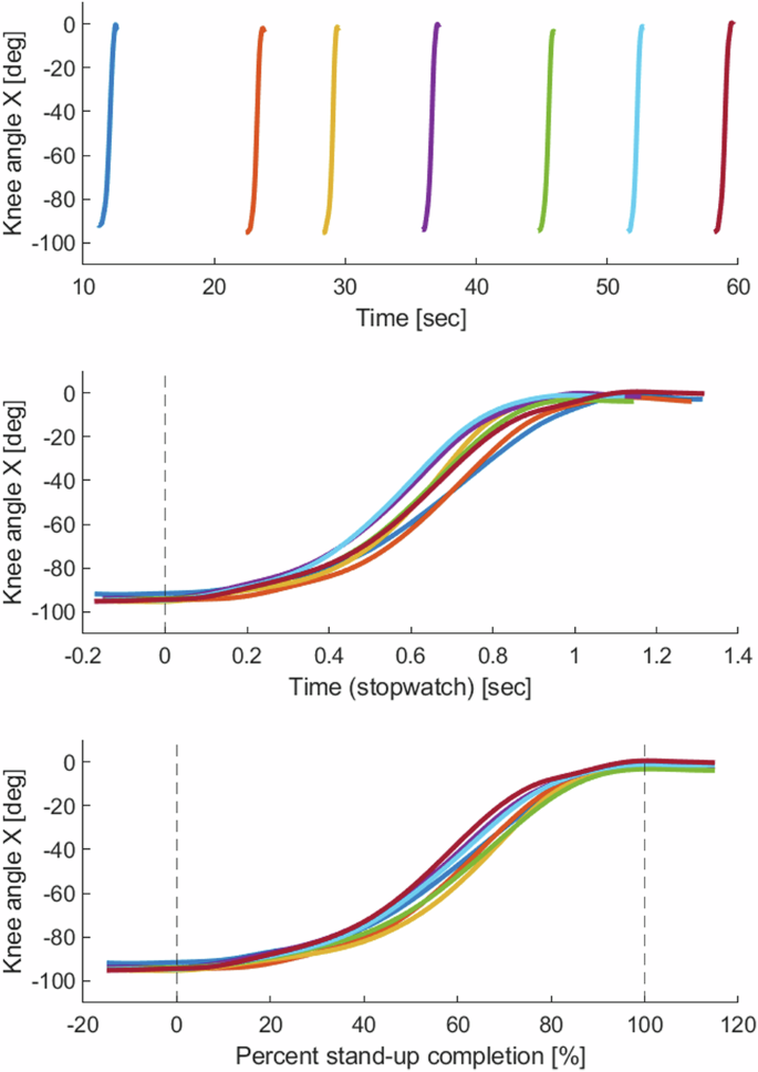
Knee position (intact-side only) from multiple repetitions vs. time, stopwatch, and percent completion. The segmentation shown is intact-side segmentation, zoomed out 30%. Top: knee angle vs. time. Middle: knee angle vs. time (stopwatch), with a vertical line showing 0% stand-up. Bottom: knee angle vs. percent completion, with vertical lines showing 0% and 100% stand-up completion.
Stopwatch: data..stopwatch, measured in seconds, is the time before and after the start of the movement. Plotting multiple repetitions vs. stopwatch will result in repetitions aligned at time = 0, with different start and stop times (0% zoom will only have different stop times; the starts will align). See Fig. 6, middle subplot. Stopwatch is created by subtracting the value of time at index_0_percent from the time vector for each repetition. For 0% zoom, the result is a vector that starts at 0 and counts up to the duration of the repetition. For higher zoom values, the first elements of each stopwatch vector will be negative. Stopwatch will equal 0 at index_0_percent. Stopwatch will equal the repetition duration (seconds) at index_100_percent and increase from there for the later part of the zoomed-out frames.
Percent completion: data..percent_completion is a vector that goes from –(zoom_percent/2) to + (zoom_percent/2). Plotting multiple repetitions vs. percent_completion will result in an “ensemble” of aligned repetitions. See Fig. 6, bottom subplot. For 0% zoom, percent_completion will equal 0 at frame 1 and equal 100 at frame 1001. For higher zoom values, for example, 30% zoom, percent_completion will start at −15% and end at 115%.
Segmented data: structure and variable details
Segmentation Info: data.segmentation_info contains multiple fields with information about the segmentation that led to the currently-open data structure: segmentation_type is a string and either equal to ‘intact_side’ or ‘prosthesis_side’. zoom_percent is a single number equal to 0, 10, 20, 30, or a different number if you have added additional zooms and re-run the data processing script. index_zoomed has parts for up, down, and full, and each contains a 2 × n vector where the first row contains the “starts” and the second row contains the “stops”. These indices are the indices used to segment the data structure that you’ve opened. If zoom_percent equals 0, the numbers will be the same as in “[SubjectCode]_start_stop_index.mat” (deleted repetitions will not be represented). If the data set has been zoomed, these numbers will be different than the index values contained in the subject folder [SubjectCode]_start_stop_index. These index values will correspond with each repetition’s frame 1 and frame 1001 in the un-segmented data. n_reps_included has parts for up, down, and full, and each contains a single number equal to the number of reps included in the structure – this value will equal “n”. This value is updated if you use remove_repetitions to remove reps (see Function: remove_repetitions). reps_with_nans has parts for up, down, and full, and each contains the fields hands, bad_gastrocnemius, bad_vastus_medialis, bad_tibialis_anterior, and bad_biceps_femoris. Each of these fields contains a vector of variable length, indicating the repetitions that will have NaNs due to each type of problem. If you’ve used “remove_repetitions.m” (see Function: “remove_repetitions.m”), the information will be updated.
Variables: subject_info
The field data.subject_info contains multiple fields with information about the subject.date is a string indicating the date of the data collection. Dates are formatted YYYYMMDD, Y = year, M = month, D = day. subjectcode is a string containing the subject code TF##. prosthesis_side is a character, either ‘L’ for left or ‘R’ for right, indicating the prosthesis/amputation side for this subject. intact_side is a character, either ‘L’ for left or ‘R’ for right, indicating the intact/healthy side for this subject. weight_kg is the subject’s weight in kg. height_m is the subject’s height in meters. EMG_labels is a dictionary that matches the sensor number to the muscle it recorded.
Variables: prosthesis_side and intact_side
Within data..prosthesis_side and data..intact_side are variables from the subject’s prosthesis side and intact side, respectively. Each listed variable will contain an n × 1001 matrix. Each of the n columns represents a repetition, and each column will contain 1001 rows representing 1001 frames. These variables can be plotted vs. data..time, data..stopwatch, or data..percent_completion, each of which is an n × 1001 matrix.
Ankle
ankle_angle_X, Y, and Z are ankle angles, with units of degrees.
ankle_torque_X, Y, and Z are ankle torques, normalized by the subject’s body weight, with units of Nm/kg.
ankle_vel_X is ankle angular velocity in the sagittal plane, with units of degrees/second.
ankle_acc_X is ankle angular acceleration in the sagittal plane, with units of degrees/(second^2).
ankle_power is ankle power (a scalar), normalized by the subject’s body weight, with units of Watt/kg.
X indicates sagittal plane. Dorsiflexion is positive, plantarflexion is negative.
Y indicates frontal plane. Inversion (medial rotation) is positive, eversion (lateral rotation) is negative.
Z indicates coronal/transverse plane. Adduction is positive, abduction is negative.
Knee
knee_angle_X, Y, and Z are knee angles, with units of degrees.
knee_torque_X, Y, and Z are knee torques, normalized by the subject’s body weight, with units of Nm/kg.
knee_vel_X is knee angular velocity in the sagittal plane, with units of degrees/second.
knee_acc_X is knee angular acceleration in the sagittal plane, with units of degrees/(second^2).
knee_power is knee power (a scalar), normalized by the subject’s body weight, with units of Watt/kg.
X indicates sagittal plane. Extension is positive, flexion is negative.
Y indicates frontal plane. Adduction is positive, abduction is negative.
Z indicates coronal/transverse plane. Internal rotation is positive, external rotation is negative.
Hip
hip_angle_X, Y, and Z are hip angles, with units of degrees.
hip_torque_X, Y, and Z are hip torques, normalized by the subject’s body weight, with units of Nm/kg.
hip_vel_X is hip angular velocity in the sagittal plane, with units of degrees/second.
hip_acc_X is hip angular acceleration in the sagittal plane, with units of degrees/(second^2).
hip_power is hip power (a scalar), normalized by the subject’s body weight, with units of Watt/kg.
X indicates sagittal plane. Flexion is positive, extension is negative.
Y indicates frontal plane. Adduction is positive, abduction is negative.
Z indicates coronal/transverse plane. Internal rotation is positive, external rotation is negative.
GRF
GRF_X, Y, and Z are the ground reaction forces, normalized by subject’s body weight, with units of N/kg.
The components of the GRF are with respect to the global/lab coordinate system. See Fig. 3 for the lab/global coordinate system for right-side and left-side amputees.
X is anterior/posterior GRF. For subjects with right amputations, who faced towards -X, a GRF vector pointing anterior will have a negative X component. For subjects with left amputations, who faced towards +X, a GRF vector pointing anterior will have a positive X component.
Y is medial/lateral GRF or left/right GRF. For subjects with right amputations, a medial-pointing R_GRF_Y will be negative, and a medial-pointing L_GRF_Y will be positive. For subjects with left amputations, a medial-pointing R_GRF_Y will be positive, and a medial-pointing L_GRF_Y will be negative.
Z is vertical GRF. It is positive.
COP
COP_X, Y, and Z are the center of pressures from a single foot. The units are meters.
COP_vel_X, Y, and Z are center of pressure velocities from a single foot. The units are meters/second.
COP_acc_X, Y, and Z are center of pressure accelerations from a single foot. The units are meters/(second^2).
COPs are labelled with respect to the global/lab coordinate system and measured from the origin of the lab coordinate system. See Fig. 3 for the lab/global coordinate system for right-side and left-side amputees.
Variables: “M”, medial
Each listed variable will contain an n × 1001 matrix. Each of the n columns represents a repetition, and each column will contain 1001 rows representing 1001 frames. These variables can be plotted vs. data..time, data..stopwatch, or data..percent_completion, each of which are n × 1001 matrices.
COM
COM_X, Y, and Z are the model center of mass positions. The units are meters.
COM_vel_X, Y, and Z are the model center of mass velocities. The units are meters/second.
COM_acc_X, Y, and Z are the model center of mass accelerations. The units are meters/(second^2).
COMs are labeled with respect to the global/lab coordinate system and measured from the origin of the lab coordinate system. See Fig. 3 for the lab/global coordinate system for right-side and left-side amputees.
COP_combined
COP_combined_X, Y, and Z are components of the “model center of pressure” or “net center of pressure” – the center of pressure derived from combining the left and right force plates. The units are meters.
COP_combined_vel_X, Y, and Z are center of pressure velocities from the combined force plates. The units are meters/second.
COP_combined_acc_X, Y, and Z are center of pressure accelerations from the combined force plates. The units are meters/(second^2).
COPs are labelled with respect to the global/lab coordinate system and measured from the origin of the lab coordinate system. See Fig. 3 for the lab/global coordinate system for right-side and left-side amputees.
Variables: EMG and EMG_raw
EMG
Each listed variable will contain an n × 1001 matrix. Each of the n columns represents a repetition, and each column will contain 1001 rows representing 1001 frames. These variables can be plotted vs. data..time, data..stopwatch, or data..percent_completion, each of which are n × 1001 matrices.
The four variables are gastrocnemius, vastus_medialis, biceps_femoris, and tibialis_anterior. Each variable has unit μ volts.
The signals in this section have been processed by band-pass filtering, rectifying (absolute value), and then low-pass filtering at 3 Hz to create an envelope. See section MATLAB Step 3 – Filter for details about the processing of the envelopes.
EMG_raw
The variables listed in EMG_raw contain n × 10010 matrices. Each of the n columns represents a repetition, and each column will contain 10010 rows representing 10010 frames.
EMG_raw contains its own time_EMG_raw, stopwatch_EMG_raw, and percent_completion_EMG_raw, which can be used to plot the EMG signals gastrocnemius, vastus_medialis, biceps_femoris, and tibialis_anterior in EMG_raw. See the function “plot_EMG.m” for an example.
EMG Normalization
The EMG and EMG_raw signals are converted from volts to μ volts before segmenting. The magnitude of the EMG envelopes and EMG_raw signals have not been normalized, so each muscle and each subject’s EMG magnitude may have a different range. Maximal voluntary contractions were not performed. Therefore, we recommend using the EMG results for non-magnitude-related analyses or magnitude comparisons within-subject and within-muscle.
Technical Validation
Motion capture system calibration
Before initializing the motion capture system, the cameras and force plates were turned on to warm up for at least 30 minutes, up to overnight. The cameras were calibrated 30–60 minutes before the experiment. If any cameras indicated that they had been “bumped”, or if we observed evidence of poor calibration, we asked the subject to exit the room while we re-calibrated the system. We initialized the motion capture cameras and force plates following the manufacturer’s instructions. We calibrated the cameras using a 5-LED Active Wand [21]. We set the volume origin by placing the calibration wand at the corner of a third “dummy” force plate [21]. We zeroed force plates first using a button on the amplifier and then zeroed them using the software Vicon Nexus before capturing trials.
Two forms of calibration error are recorded for each camera in the “.xcp” file for each trial: image error, measured in pixels, and world error, measured in mm. The xcp file can be opened using a text editor. All processing performed in Vicon Nexus is recorded in the “.history” file for each trial.
Electromyography
We placed Delsys Trigno Avanti electromyography (EMG) electrodes on the skin over the subjects’ intact-side muscles following SENIAM placement procedures and after preparing the skin by shaving and wiping with alcohol24. We wrapped the EMG sensors with elastic co-adhesive wrapping (CobanTM) and/or adhesive kinesiology tape (KT-TapeTM) to ensure contact between the electrodes and skin.
To determine the quality of the EMG signals, two researchers with experience using and processing EMG signals visually inspected the raw signals and the envelopes to evaluate whether large “spikes” were likely to be true signal or likely to be artifact. Repetitions that were likely to contain artifact were removed based on the consensus of both researchers. The full, raw signals are included in the files that precede the “segmented” data files, and researchers may modify which repetitions are excluded by changing the index values identified in Step 0 of each subject’s “[SubjectCode]_processing.m” script, and rerunning the script to re-process the results.
Use of hands
We asked all subjects to stand up and sit down without hands if possible. However, some subjects were unable to stand up or sit down without using their hands on the chair’s armrests. We watched the video recordings and 3D reconstructions of the trials in Visual 3D to identify repetitions when the subjects used their hands. Because the chair we used was not instrumented with force-torque sensors, force-based measurements are inaccurate. In particular, the Center of Pressure (COP) and joint torques and powers are invalid. During repetitions when subjects used hands, therefore, we replaced these variables with “NaN” to avoid accidental inclusion in the analysis. The Ground Reaction Forces (GRF) are also not fully representative of the force exerted by the subject on the environment during these repetitions, but we did not replace the GRF with NaN during repetitions with hands. We made this decision because the GRF in this situation will be underestimated but not completely erroneous or misleading (as in the case of COP, torque, and power). The GRF information can still be valuable to researchers in this situation, and we do not believe there is a risk of significant misinterpretation of the data from the GRF during these trials.
Usage Notes
Vicon
To open the Vicon database, download the ViconDB_STS folder to your computer. ViconDB_STS folder should be a “Patient Classification” (green circle) inside of your main Vicon “Database”. Open Vicon Nexus. If you do not see the Communications panel, click Window and then Reset to Default Layout. In the Communications panel, click Data Management. If needed, select your database – choose the folder “above” ViconDB_STS. The folder ViconDB_STS and all of the folders inside of it contain.enf files. The.enf file identifies the hierarchy of the database within Vicon Nexus, and identifies a Database, a Patient Classification, a Patient, and a Session.
To give Vicon access to the model files, save them into the following folder on your computer: C:UsersPublicDocumentsViconNexus2.xModelTemplates
To give Vicon access to the pipeline files, save them into the following folder on your computer: C:UsersPublicDocumentsViconNexus2.xConfigurationsPipelines
Note: you may need to change the slashes from to /, depending on your operating system.
MATLAB: Example code and helpful functions
Several scripts with example code are included to demonstrate how to load files, loop through the structures, and plot the variables. The example code also demonstrates the use of the helpful functions. The scripts are included in the main MATLAB_STS folder and should be run from that folder. The functions are included in the folder functions_STS_DB and can be called from any folder, as long as the folder “MATLAB_STS/functions_STS_DB” is on the MATLAB path. The folder is added to the path at the start of each example script.
Function: “variable_xyz_unit.m”
Description
This function will convert a variable name into the components of a “nice” label – for example, the input ‘knee_angle_X’ will return up to four outputs: [‘Knee Angle X [deg]’, ‘Knee Angle’, ‘X’, ‘[deg]’]. Writing a single output will return the full label, ‘Knee Angle X [deg]’. This function is nice for creating titles or y labels. The units are correct for the segmented data as published.
Inputs
variable – (string), a string of the variable name from the structure. For example, ‘knee_angle_X’.
Outputs
ylabel_string – (string), the nicely written label with all three parts and spaces in between. For example, ‘Knee Angle X [deg]’. If you only assign one output, this is the output you’ll get. Assign more than one output if you want separate components.
varname – (string), the name of the variable, without underscores, capitalized, and with partial words like “vel” and “acc” written out fully.
xyz – (string), either ‘X’, ‘Y’, ‘Z’, or empty ‘’ if the variable does not have X, Y, or Z in the name.
unit – (string), the unit of the variable (as published), with brackets.
Where to find examples
The example script “Figures_shift_zoom_segs_times.m” uses it two ways:
> ylabel_string = variable_xyz_unit(‘knee_angle_X’);
> ylabel(ylabel_string)
> ylabel(variable_xyz_unit(‘knee_angle_X’))
See Example script: “Figures_zooms_segs_times.m”
The function “plot_one_variable.m”, see Function: “plot_one_variable
Function: “plot_one_variable.m”
Description
This function plots a single variable from a single side for all three parts of the movement. Up, down, and full are on separate subplots, and every repetition of the variable included in data is plotted. See Fig. 8 – both plots are created using “plot_one_variable.m”.
The colors and lines use the line styles of the “plot_after_segmentation.m” function where repetitions 1–7 are solid lines with different colors, and repetitions 8–16 repeat the same 7 colors but with dashed lines.
Inputs
data – (struct) – structure containing segmented data, with fields up, down, full, segmentation_info, and subject_info.
side – (string) – the side you want to plot: either ‘intact_side’, ‘prosthesis_side’, ‘M’, ‘EMG’, or ‘EMG_raw’.
variable – (string) – a variable that exists in the structure for the side specified.
Outputs
A new figure is created (not an output)
fig_handle – the figure handle so you can resize the figure if you want.
Where to find examples
Inside of the function “remove_repetitions.m”, see Function: “remove_repetitions.m”
Function: “remove_repetitions.m”
Description
This function will remove repetitions from the segmented data for one subject (delete the repetition’s column from all signals in the structure), either based on the repetition index number(s), or based on when subjects used hands, or when an EMG signal was bad.
We recommend reading the comments in “Example_Remove_Repetitions.m” and running each section to see the examples.
Inputs
data – (struct) – structure containing segmented data, with fields up, down, full, segmentation_info, and subject_info.
remove – (struct) – structure with the following fields, indicating which repetitions to remove. It has fields remove.rep_number, which is a vector of numbers indicating specific repetition index numbers you want to remove, and five binary fields: remove.hand, remove.bad_gastrocnemius, remove.bad_tibialis_anterior, remove.bad_biceps_femoris, remove.bad_vastus_medialis. If any of these fields are set equal to 1, columns with that type of “bad rep” will be removed.
parts_to_remove – (cell array of strings) – a cell array of strings, for example {‘up’, ‘down’, ‘full’} to remove reps from all parts, or {‘up’, ‘full’} to only remove reps from up and full.
plotson – (1 or 0), indicate whether you want a plot of the knee angle before and after deletions. An example of the plots is shown in Fig. 8.
Outputs
data – (struct) a structure with the desired repetitions removed and the segmentation_info updated. The fields will be up, down, full, segmentation_info, and subject_info.
Where to find examples
“Example_Remove_Repetitions.m” Example script: “Example_remove_repetitions.m”
Example script: “example_remove_repetitions.m”
This script contains example inputs for “remove_repetitions.m”, warnings, and examples. It should be run from within the MATLAB_STS folder. The first section includes detailed explanation of each input. The examples demonstrate the functionality of the remove_repetitions function and how to use it with subjects TF03 and TF07, who had a repetition of “down” and “full” deleted without the corresponding “up” being deleted. The sections of this script are as follows:
Section 1: Explanation of inputs
Example 0: All of the inputs, less comments. For copy-pasting to use.
Example 1: Delete specific repetitions (easy – subjects with even # of reps in each part)
Example 2: Delete a repetition (hard – subjects with uneven # of reps)
Example 3: Delete repetitions when the subject used hands
Example 4: Try deleting a repetition that is out of range
Example 5: Try deleting all of the repetitions
Example script: “Single_subject_plots.m”
This function creates three figures for each subject: a stand-up figure showing lower limb joint angles, torques, and power, a sit-down figure showing lower limb joint angles, torques, and powers, and a figure showing the EMG envelopes. These figures show the segmented data sets without removing any additional repetitions. The function saves three figures per subject into the folder “MATLAB_STS/Figures”.
Example script: “Figures_zooms_segs_times.m”
This function creates the figures Figs. 4–6.
MATLAB: hints, troubleshooting
Structure arrays
Overview of structure arrays
The MATLAB results are stored inside of structure arrays, a type of MATLAB variable that allows for “nesting” variables inside of “fields”. In this section, we’ll refer to one of the segmented data structures.
Any type of variable can be contained in a structure array. The variables are contained at the terminal ends of branches within the structure. See Fig. 7 for the “branches” of the segmented data structure.
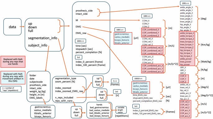
Organization of the segmented mat structure. Dimensions (ex. 2 × n) and units in [brackets] are included where appropriate. n is the number of repetitions included in a part of the data structure. The number n may be different in different parts, for example, “up” and “down” may have different n’s.
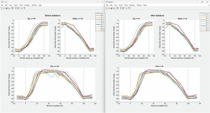
The output of Example1 of “Example_remove_repetitions.m”, removing repetition 8. Left: before deletions. Right: after deleting repetition 8. The figures are created using “plot_one_variable.m”.
Loading a structure
If you double-click on the mat file to open it or call it using load(‘filename’) without assigning an output, the name data will appear in your workspace. It will have fields up, down, full, subject_info, and segmentation_info. To call any of these variables, you need to use the full structure reference: data.up, data.down, etc).
If you open the structure using the code D = load(‘filename’), the workspace will have a variable named D with a single field, D.data, and D.data will have the fields up, down, full, subject_info, and segmentation_info. Continuing from the example above, you can remove the outer layer of the structure using the code “data = D.data” will result in the workspace variable data with the fields up, down, full, subject_info, and segmentation_info.
Workspace variable – renaming
Continuing from above, you can rename the main variable similarly; “data2 = data” will result in a variable data2 with the same fields as data.
Combining structures
Say we have segmented files from three subjects saved in our workspace as follows:
Data_TF01 with the fields up, down, full, subject_info, and segmentation_info.
Data_TF02 with the fields up, down, full, subject_info, and segmentation_info.
Data_TF05 with the fields up, down, full, subject_info, and segmentation_info.
Here are two examples of ways we could combine them:
Example 1:
Data.TF01 = Data_TF01;
Data.TF02 = Data_TF02;
Data.TF05 = Data_TF05;
The resulting structure Data will have three fields: TF01, TF02, and TF05. Each of the subfields (ex. Data.TF01) will have fields up, down, full, subject_info, and segmentation_info.
Example 2 (does not continue from Example 1)
Data.up.TF01 = Data_TF01.up;
Data.up.TF02 = Data_TF02.up;
Data.up.TF05 = Data_TF05.up;
The resulting structure Data will have one field: up. Data.up will have the fields TF01, TF02, and TF05. The fields of Data.up.TF01 will be the fields originally contained in Data_TF01.up (intact_side, prosthesis_side, M, etc)
Fieldnames function
The MATLAB built-in function fieldnames will return a cell array of strings of the fields. In Example 2 above, “fieldnames(Data)” will return the cell array {‘up’}. “fieldnames(Data.up)” will return {‘TF01’, ‘TF02’, ‘TF03’}. You can also create similar cell arrays by typing them into the script.
Loops
You can loop through any of the fields in a structure. This makes processing the data much more streamlined. This example will continue from Example 2 above and plot the variable knee_angle_X for the three subjects:
subjects = fieldnames(Data.up); % use fieldnames to find the fields
for S = 1:length(subjects)
plot(Data.up.(subjects{S}).knee_angle_X)
end
Other examples of using loops and structures are included in the example code and in the functions.
Expected fields
In the MATLAB functions included with the dataset, when a structure is an input to the function, we have specified “expected fields”. This will be the fields within the structure that the function expects to find. Only the first layer of fields is described in functions.
System compatibility
It’s possible that your system could cause problems running the included code. The following problems are the ones we have predicted. The code was written and executed in MATLAB R2022b on a Lenovo ThinkPad laptop running Windows 11 Enterprise version 23H2 OS build 22631.3593.
File paths ( vs /)
Mac computers may require different slashes in the file paths.
Set position (figures)
Many of the figures are positioned on the screen using the “set” function. If the figures appear tiny or off-screen, comment out the instances of “set”, Alternatively, move and size the figure as desired, then use the following code to get the position: “get(gcf, ‘position’)”. Four numbers will appear in the command line. Apply them using “set(gcf, ‘position’, [# # # #])”.
Set position (legends)
Similarly, many of the legends are positioned using the “set” function. If the legends are not where you like them, comment out the line that sets the legend handle. Alternatively, move the legend where you want, right-click and choose “properties”, then drop down the first section to find the position property. Copy the numbers. Use them with the line of code “set(legend_handle, ‘position’, [# # # #])”.
MATLAB version
To use the included code, you need at least version R2018b, which includes the function sgtitle. Alternatively, when you run into errors about sgtitle, comment out that line, or replace it with the function suptitle. sgtitle creates a larger title above subplot titles.
Required functions, packages, add-ons
The following function needs to be downloaded from external sources:
cell2csv.m: https://www.mathworks.com/matlabcentral/fileexchange/47055-cell-array-to-csv-file-improved-cell2csv-m
We are not aware of any additional packages or add-ons that are required.


Responses