Risk-constrained participation of virtual power plants in day-ahead energy and reserve markets based on multi-objective operation of active distribution network

Motivation

Deploying renewable energy sources (RESs), such as photovoltaic (PV) and wind systems (WS), is a highly effective strategy for minimizing distribution network operating costs while ensuring a sustainable energy supply. These sources are characterized by minimal environmental emissions and low energy generation costs¹. However, the electricity generation from RESs is inherently unpredictable due to its dependence on climatic conditions and potential inaccuracies in weather forecasts².

The limited flexibility of energy networks integrating RESs leads to inconsistencies in real-time (RT) and day-ahead (DA) operations, potentially causing supply–demand imbalances in real-time scheduling². Furthermore, high penetration levels of these sources may result in overvoltage issues, potentially compromising the insulation of equipment³. To address these challenges, incorporating flexibility sources such as energy storage systems (ESSs) and demand response programs (DRPs) is essential⁴. Establishing an energy management system (EMS) requires the presence of an effective aggregator and coordinator for various resources, such as a virtual power plant (VPP)⁵. With efficient energy management, a VPP can harness the benefits of RESs and flexibility to achieve financial gains by trading energy in the market and offering diverse ancillary services. Additionally, optimal scheduling and coordination between VPPs and the distribution system operator (DSO) can enhance the operational performance of the distribution network.

Literature review

Extensive research has been conducted on optimal VPP operation and energy management strategies. Conditional value-at-risk (CVaR) has been employed to reduce profit risk, offering the optimal bidding strategy for hybrid power plants in intraday and daily markets⁶. CVaR, also known as expected shortfall, is a risk measure that quantifies tail risks by calculating the weighted average of “extreme” losses beyond the value-at-risk (VaR) threshold. This measure is widely used in portfolio optimization for effective risk management⁶. Stochastic tendering strategies for VPPs with ESSs and DRPs have been proposed to enhance WS profitability in short-term power markets⁷. A distributed clustering approach introduced in⁸ determines ESS membership in VPPs based on ESS size and owner preferences. The integration of electric vehicles (EVs) within a VPP was shown to smooth wind power output⁹. For VPPs with PV and WS, power management strategies have been implemented to facilitate energy market participation¹⁰. Reference¹¹ presented a storage system model integrated into a VPP to enhance generation adequacy and comply with energy management requirements. High penetration of RESs and non-flexible loads often leads to power flow exceeding distribution line limits, causing congestion in distribution networks. VPPs effectively combine various energy sources to increase RES penetration and mitigate these challenges¹².

Bi-level programming has been used to manage active distribution networks (ADNs) with multiple VPPs. In this framework, the upper level minimizes ADN operational costs while considering market dynamics, system security, and economical operation. The lower level maximizes VPP profits by leveraging flexible resources¹³. In Ref.¹⁴, a DA self-scheduling model for VPPs participating in reserve and energy markets was proposed. The model incorporated conventional power plants, ESSs, WSs, and variable demand, while addressing uncertainties in market prices and WS output. Reference¹⁵ introduced an energy management model for smart distribution networks with flexible-renewable VPPs participating in DA markets. The upper layer maximizes VPP profits through efficient coordination of renewable and flexible sources, while the lower layer focuses on minimizing energy losses and voltage variations by coordinating VPP operations with the DSO.

In Reference¹⁶, a VPP configuration was proposed to aggregate residential batteries and EVs, managing their charging and discharging processes to control bus voltages and alleviate transformer loading. This strategy ensures batteries are fully charged during the day using solar and grid power. Reference¹⁷ proposed an optimized operational scheduling framework for VPPs integrating solar, wind, and fuel cell units with co-generation systems to address power shortages due to renewable sources. Reference¹⁸ expanded this concept by forming a network of flexible resources within a multi-area interconnected system. A three-step voltage regulation coordination framework is introduced in Ref.¹⁹, leveraging a Data-driven Robust Optimization method with a Wasserstein metric ambiguity set for active and reactive power adjustments. Reference²⁰ explored VPP scheduling optimization within the energy internet framework, using a multi-objective PSO algorithm to improve the success rate of the proposed method.

Table 1 shows the taxonomy of the research literature in this field.

The following research gaps in VPP energy management within distribution networks have been identified based on the research background and Table 1:

• VPPs serve as coordinators for energy sources, ESSs, and responsive loads. By effectively managing these resources, VPPs can significantly enhance the voltage profile and reduce operational costs, thus improving both the technical and economic aspects of the network. Consequently, sources, ESSs, and responsive loads are expected to achieve financial benefits by participating in energy and ancillary service markets. However, most research focuses on energy market models, while ancillary service market models, such as reserve regulation, are explored in only a limited number of studies (e.g.,^14,15). Additionally, the acquisition of financial benefits is contingent upon a risk model which are rarely considered, as demonstrated by⁶.

• When analyzing the performance of distribution networks with VPPs, most studies integrate VPP objectives (e.g., optimal market participation) with distribution network goals (e.g., operational cost reduction). However, VPPs and networks may have distinct and sometimes conflicting requirements. Therefore, the system necessitates a multi-objective or bi-level optimization approach. This has been addressed in only a few studies (e.g.,^5,13,15).

• The operation of distribution networks with VPPs is typically addressed using nonlinear programming (NLP) or mixed-integer NLP (MINLP) frameworks. Linear approximation models are commonly employed (e.g.,^{5,10,11,13,15}) using linearization techniques and solvers like Simplex. However, this approach may introduce computational errors of up to 10% in network loss calculations⁵. Non-hybrid evolutionary algorithms (NHEAs), such as genetic algorithm and particle swarm optimization, have been proposed to address these limitations^9,12]. However, their solutions often lack uniqueness. Hybrid evolutionary algorithms (HEAs) are crucial for addressing this issue due to the need for updating decision variables in several processes to solve the problem²¹.

Contributions

This study investigates the role of flexible-renewable VPPs in energy and reserve markets within active distribution networks, addressing the research gaps identified earlier. The presented approach improves both the technical and economic aspects of ADNs by coordinating energy sources, ESSs, and responsive loads within a VPP framework. A bi-level optimization approach is employed, where the upper level determines the optimal scheduling of the ADN by minimizing operating costs and voltage deviations using weighted functions based on Pareto optimization. The AC optimal power flow equations, which include power flow and operational constraints, govern this level. The lower level is designed to maximize the expected profits of VPPs while incorporating the CVaR model for risk management. The reserve and operational constraints of VPPs, including renewable energy sources and DRPs, are also taken into account. A stochastic programming model integrates the Kantorovich Method and the Roulette Wheel Mechanism to address uncertainties related to renewable power generation, load, and market prices. To ensure reliable and nearest optimal solution, the study employs a hybrid SCA + TLBO algorithm, which reduces computational variance and overcomes the limitations of previous methods. The main contributions of this study are summarized as follows:

• Financial benefits for energy sources and responsive loads in flexible-renewable VPPs through participation in day-ahead energy and reserve markets, with consideration of the CVaR model.

• Simultaneous achievement of the DSO’s operational goals and VPP owners’ economic objectives using a bi-level multi-objective optimization framework.

• Achieving reliable and optimal solutions with minimal deviation using the hybrid SCA + TLBO algorithm.

Paper organization

The structure of this document is as follows: The bi-level and single-level stochastic models of the presented method are described in Section “ADN operation in the presence of the flexible-renewable VPPs”. The application of the hybrid SCA + TLBO method to tackle the presented issue is described in Section “Solution procedure”. Finally, Sections “Numerical results and discussion” and “Conclusion” provide the numerical findings and conclusions, respectively.

Bi-level model

This section discusses how to schedule an ADN using flexible-renewable VPPs. The proposed scheme for ADN operation is illustrated in Fig. 1. As shown, the risk model (CVaR) is utilized to account for VPPs’ participation in the DA reserve and energy markets. With the top-level ADN energy management aimed at reducing operating costs and the voltage deviation function (VDF) under OPF equations, the proposed approach is structured as a bi-level optimization model. Additionally, the objective of VPP participation in the aforementioned markets is to maximize profitability while considering constraints related to the integration of RESs and flexibility in the lower-level problem.

Proposed scheme for ADN operation in the presence of the flexible-renewable VPPs.

Full size image

In this paper, the operational aims of the DSO are considered in the upper-level problem. These objectives include minimizing network operating costs and the VDF. By minimizing the VDF, the voltage drop across distribution lines is expected to decrease, which would subsequently minimize power and energy losses. The economic objective of VPPs is addressed in the lower-level model, where the VPP operator’s objective function is introduced as profit maximization.

The mathematical model for the proposed technique is presented below.

Subject to:

Subject to:

A more advanced formulation is provided in (1)–(9). The objective function, defined in Eq. (1), seeks to minimize the estimated cost of energy procurement by the ADN from the upstream network (OC)²² and the VDF²³, formulated as a bi-objective optimization model. This connection is established using the Pareto optimization methodology, based on the weighted sum method, which requires the sum of the weight coefficients ω_OC and ω_VDF to always equal one²⁴. The Pareto front of the proposed scheme is depicted in a two-dimensional coordinate system, reflecting the distinct OC and VDF function values generated by varying weight coefficients²⁴. This method enables identifying the lowest and highest values of the respective functions under two scenarios: ω_OC = 1 and ω_VDF = 1. The Fuzzy Decision Algorithm (FDA) detailed in Algorithm 1⁴, is employed to determine the optimal solution, which represents a compromise between the different objectives.

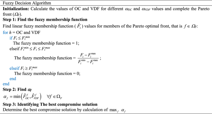
The pseudo-code of the FDA.

Full size image

Constraints (2)–(9), which represent the ADN’s operational limitations²⁵, define the AC-OPF of the ADN. The AC power flow equations (AC-PF) are described in (2)–(6)^22,23. The active power balance at each bus of the network is defined in (2), while the reactive power balance is presented in (3) ^26,27,28,29. Equations (4) and (5) determine the active and reactive power flows in the distribution lines, respectively. The voltage angle at the reference bus is specified in Eq. (6)^30,31,32. Additional operating constraints include the capacity of lines (7), the apparent power limit of distribution substations (8), and the bus voltage amplitude limits (9). These constraints ensure the maximum allowable apparent power through substations and distribution lines. Upper and lower voltage limits are implemented to prevent equipment insulation damage due to overvoltage and consumer outages due to high voltage drops. The ADN is linked to the upstream network via a distribution substation located at the reference bus, while P^G and Q^G are set to zero for all other buses.

The lower-level problem is formulated in Eqs. (10–19). Equation (10) represents the objective function, which is divided into two components. The first component addresses the expected profits of VPPs in the DA reserve and energy markets. The profit is calculated by multiplying the market price with the active or reserve power provided by the VPP. If P^VPP is positive, the VPP benefits from the specified energy market. Conversely, if P^VPP​ is negative, the VPP must pay for the energy consumed in consumer mode. Interestingly, since reserve power is provided in response to network requests made by the VPP, it is always positive, ensuring that VPPs benefit from the reserve market. The second component of Eq. (10) incorporates the CVaR-based risk model⁶, where the coefficient β reflects the VPP’s risk aversion in these markets. A higher β value indicates greater risk aversion. Furthermore, Eqs. (11) and (12) define the CVaR and reveal risk constraints⁶.

Constraints (13)–(19) present the operational model of VPPs utilizing RESs and DRPs. The imbalance between the active power produced and consumed within VPPs can either be stored as a reserve or delivered as active power to the ADN¹⁴. In essence, the total active power and reserve of a VPP are equal to the sum of the active power generated by renewable resources and demand response, minus the active power consumed by the load. This determines the power balance constraint in VPPs. Constraint (14) defines the active power generated by RESs^33,34.

The maximum power output of an RES, represented by P^max​​, depends on climatic variables such as solar radiation and wind speed. RESs are expected to operate at their maximum power output during all operational hours because of their minimum operating costs and emissions^35,36. Equations (15), (16) form the foundation of the incentive based DRP model³⁷. DRP participants can adjust their energy consumption based on market price signals. Consumers are encouraged to increase energy usage during off-peak hours with lower prices and decrease it during peak hours with higher prices. Constraint (15) defines the range of variations in consumers’ active power, while constraint (16) ensures that their energy will stay constant during the operating horizon regardless of how much it increases or decreases. Finally, constraint (17) limits the active power exchanged between the VPP and ADN due to line and substation capacity restrictions. The maximum reserves available to VPPs are determined by constraints (18) and (19)¹⁴.

Single-level model

Equations (1–19) introduce the bilevel version of the optimization problem. Such optimization models are typically solved by classical solvers, starting with an integrated single-level model. Since the lower-level problem involves linear equations, it is a convex model. Here, the KKT technique is employed to derive a single-level version for the proposed system³⁷. This approach entails formulating the Lagrange function (L) for the lower-level problem, which comprises the objective function (10) along with the penalty terms corresponding to constraints (11)–(17)³⁷. For constraints of the forms a ≤ b and a = b, the penalty functions take the forms μ.max( 0 , b − a) and λ × (a − b)³⁷. Here, Lagrange multipliers are represented by λ and μ. The single-level problem is formulated by integrating the upper-level objective function with the constraints derived from “equalizing the derivatives of the Lagrange function with respect to the lower-level variables and the Lagrange multipliers to zero”³⁷. Consequently, the proposed plan is defined as follows:

Subject to:

The upper-level problem (1) and the single-level formulation of optimal ADN scheduling in the presence of flexible-renewable VPPs share the same objective function, presented in (20). Based on constraint (21)³⁷, the upper-level constraints (2)–(9) are also incorporated. Constraint (22) is derived of ∂L/∂λ = 0 and ∂L/∂μ = 0, which yield the lower-level constraints (11)–(19). Equations (23)-(28) are obtained by equalizing the derivatives of the Lagrange function with respect to variables of the lower-level problem i.e., z, var, P^VPP, R^VPP, P^RES, and P^DR to zero, respectively. It is noteworthy that ∂L/∂μ = 0 results in a ≤ b and μ.(a − b) = 0³⁷. The term a ≤ b was extracted in constraint (22), and μ.(a − b) = 0 for different inequality constraints is given in (29)–(35). Finally, the boundary conditions of the Lagrange multipliers are specified in (36).

Uncertainties modeling

In the proposed scheme, several parameters are uncertain, including market prices (ρ^E and ρ^R), the maximum power generated by RESs (P^max), and active and reactive demands (P^D and Q^D). To address these uncertainties, this study adopts a stochastic programming approach, combining roulette wheel mechanism (RWM) and Kantorovich method (KM). First, RWM creates numerous scenarios according to the average and standard deviation of each scenario. To estimate market prices and load probabilities the normal probability distribution function (PDF) is used³. For maximum power generation (P^max), the Beta and Weibull PDFs are applied to PV and WS sources, respectively⁴. The probability of each scenario (π⁰) is calculated by multiplying the probabilities of its individual parameters.

At the subsequent stage, KM as a scenario reduction method reduces the number of scenarios by selecting those that are minimally different from one another. The formulation for this reduction method is detailed in⁶. Finally, the probability of a scenario after reduction is recalculated as the ratio of π⁰ for that scenario to the sum of π⁰ values for KM scenarios.

An NLP framework is implemented for solving problems (20)–(36). This section uses a combined SCA³⁸ and TLBO³⁹ algorithm to resolve the final research lacuna expressed in Section “Research gaps”. This solver minimizes the standard deviation of the final solution with respect to NHEAs, enabling it to achieve the nearest optimal solution. Its performance is evaluated in Section “Determining the best compromise solution between multi-criteria objectives of the DSO”.

The presented solver categorizes variables into two groups: decision-making and dependent variables. Decision variables in the proposed scheme include P^DR, R^VPP ​, and the Lagrange multipliers (λ and μ). The amount of these variables are obtained using the SCA + TLBO method in accordance with constraints (37)–(39). Dependent variables include P^G, Q^G, P^L, Q^L, V, θ, P^VPP, and P^RES​. The algorithm first calculates P^VPP and P^RES using Eqs. (11) and (12). The remaining dependent variables are then determined according to AC-PF Eqs. (2–6). The forward–backward method is employed to solve the problem of AC-PF⁴⁰.

The fitness function is calculated using the dependent and decision variables. The problem’s constraints (i.e., ADN operational limits (7–9), DRP constraint (16), VPP size limits (17) and (18), and KKT constraints (23–35)) are considered using a penalty function approach¹⁶. In this method, the fitness function (40) is equal to the sum of the objective function (20) and the total penalty functions (PeF), defined in Eq. (41). For constraints of the form a = b (e.g., constraints 16, 23–35), the penalty function is κ.(a—b), while for constraints a ≤ b (e.g., constraints 7–9, 17–18), it is expressed as ξ.max(0, b—a). Here, κ ∈ (-∞, + ∞) and ξ ≥ 0 are Lagrange multipliers optimized by the SCA + TLBO algorithm.

Figure 2 shows the steps of the presented technique to address the problem (20)–(36). As seen, the SCA + TLBO algorithm begins by generating N solutions to the problem, consisting of the values of the decision variables and the Lagrange multipliers (κ and ξ). The fitness function and dependent variable values are subsequently determined. The SCA + TLBO procedure optimizes the fitness function (minimizes objective function (20)) by iteratively updating the decision variables. The updating process is carried out by SCA first, followed by TLBO. Convergence is assumed upon reaching the maximum number of iterations (I_max​).

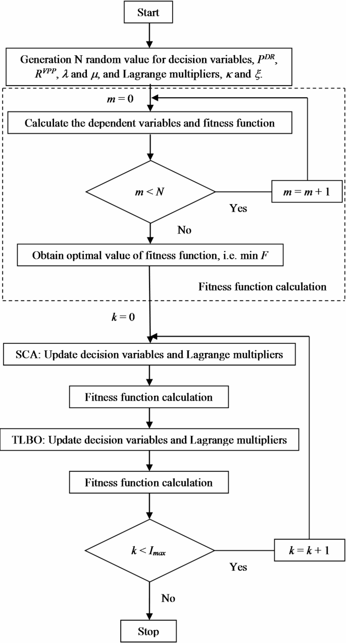
Flowchart of the presented algorithm.

Full size image

Problem data

This section presents the implementation of the presented methodology on a 119-bus ADN, as illustrated in Fig. 3⁴¹. In this network the base voltage is 11 kV and the base power is considered 10 MVA. The permissible voltage amplitudes in this network range from 0.9 to 1.1 p.u.^42,43,44. The reference bus voltage is set to 1 p.u. with a phase angle of zero radians. Detailed specifications of the distribution substation and lines are available in reference⁴¹. Demand data of the system can be obtained from reference⁴¹, while hourly demand is derived by applying the daily demand factor curve to the maximum demand values⁴⁵. This curve is presented in reference³. Energy and reserve prices are fixed at 30 $/MWh, 24 $/MWh, and 16 $/MWh, for the periods 17:00–22:00, (8:00–16:00 and 23:00–00:00), and 1:00–7:00, respectively¹⁵. This autonomous driving network includes buses 4, 11, 19, 34, 55, 67, 80, 90, 101, and 114, each equipped with ten VPPs. Each VPP consists of 0.8 MW of WS and 0.6 MW of PV systems. The active power generated by these sources is calculated as the product of their capacities and the daily power generation profile, with the WS and PV generation curves documented in reference¹⁵. Among VPP users, 40% actively participate in the DRP. Additionally, a 0.8 MW distribution line connects the VPP to the ADN bus. The calibrated value of α for the CVaR is set to 0.95⁶. The standard deviation for the three uncertainty factors in this study is 10%. The proposed method is applied to a selection of 50 scenarios out of the 2000 scenarios generated using the RWM and KM techniques.

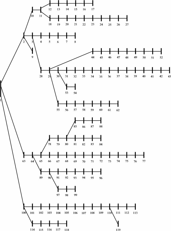
IEEE 119-bus ADN⁴¹.

Full size image

Results

The proposed method was implemented and simulated in the MATLAB software environment using the data from Section “Problem data” and the steps outlined in Section “Solution procedure” to solve the problem. A detailed report of the numerical findings is provided below.

Determining the best compromise solution between multi-criteria objectives of the DSO

The Pareto front for the DSO’s objectives which are the minimization of OC and VDF is shown in Fig. 4 for varying load levels. In this figure, the equation ω_VDF = 1 − ω_OC is maintained, and ω_OC ​ is varied from 0 to 1 in increments of 0.05. It is evident from the figure that as ω_OC increase, the importance of minimizing the expected operational cost of the ADN in the DSO’s objective function (Eq. 1) increases, while the importance of minimizing the voltage deviation decreases. Consequently, when ω_OC = 1, the minimum (maximum) value of OC (VDF) is achieved. Conversely, when ω_OC is lower than ω_VDF, the reverse is true. This asymmetry in the behavior of OC and VDF at different load levels stems from the need to add more power from local sources in the ADN—such as the VPP in this case study—to reduce OC. However, this can lead to overvoltage at certain ADN buses, increasing the VDF. At a 100% load level, the minimum (maximum) values of OC and VDF are approximately $4007.3 ($4602.9) and 6.72 (12.45) p.u., respectively. Additionally, as load levels increase, both operating costs and voltage drops rise, shifting the Pareto front curve upward and to the right (Fig. 4). Under these circumstances, the OC and VDF functions rise as a result.

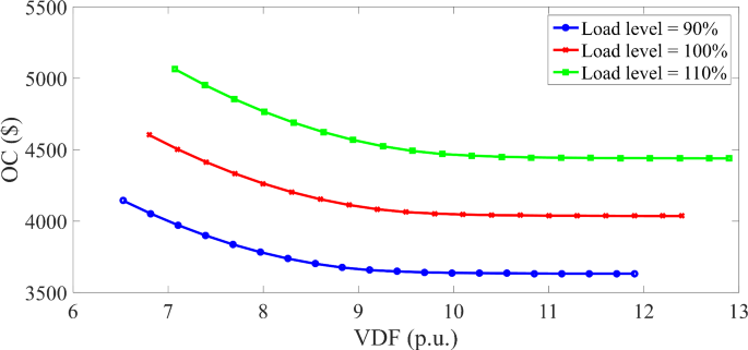
Pareto front of the proposed scheme for different load levels.

Full size image

Table 2 summarizes the best trade-offs between the DSO’s multi-criteria objectives (OC and VDF) for different load levels, as obtained using SCA + TLBO, SCA, TLBO, particle swarm optimization (PSO)²⁰, and genetic algorithm (GA)²¹. For all methods, the population size (N) and the maximum number of iterations (I_max) were set to 80 and 5000, respectively. The remaining parameters for each approach are provided in^20,21,38,39. Each algorithm was run 30 times to compute statistical indices, such as the standard deviation (SD) of the final solution.

Table 2 demonstrates that the hybrid SCA + TLBO approach achieves the lowest OC and VDF values in the shortest computation time (CT) and convergence iterations (CI) at all load levels compared to the non-hybrid SCA, TLBO, PSO, and GA algorithms. At a 100% load level, the SCA + TLBO algorithm finds the optimal solution after 2162 iterations and 178.1 s, while the other methods require more than 2730 iterations and 220 s. Furthermore, the hybrid solver has the lowest SD, around 0.95%, across different load levels, whereas the SD for other solvers exceeds 1.5% and shows larger fluctuations with load level variations. This indicates that the SCA + TLBO algorithm consistently provides nearly optimal solutions (almost unique optimal solution) due to its low SD values. However, this behavior is not observed in other methods.

The solution space for the proposed problem decreases proportionally to the load level as the load increases. This leads to a reduction in the convergence rate and an increase in CI and CT. At the optimal compromise point (OC = 0.3, VDF = 0.7) and 100% load level, the SCA + TLBO algorithm achieves OC and VDF values of $4153 and 8.61 p.u., respectively. Comparing these results with Fig. 4 reveals that the OC function is approximately 24.5% higher than its minimum value at a 100% load level ($4007.3), while the VDF function is about 33% away from its minimum value. This demonstrates that the proposed method yields values for the DSO objectives at the optimal compromise point that are close to their respective minima. As the load level increases, the Pareto front shifts upward and to the right, resulting in higher OC and VDF values and moving the optimal compromise point accordingly. This is illustrated in Fig. 4 by an increase in OC and a decrease in VDF.

In general, combining different algorithms can lead to desirable optimal solutions. In this study, the combination of TLBO and SCA was employed because, as shown in Table 2, these algorithms individually produce suitable solutions for the proposed problem. Additionally, they do not require tuning parameters, making them unaffected by problem size changes.

Performance evaluation of VPPs:

The expected daily curve of renewable sources and responsive loads in VPPs for β = 0.5 is shown in Fig. 5. According to Eq. (14), RESs such as WS and PV inject active power at their maximum capacity into the network or the VPP based on weather conditions, due to their low emissions and operating costs. This behavior is supported by Fig. 5a. As described in¹⁵, the PV power production rate reaches its maximum at 12:00, allowing it to inject up to its full capacity of 6 MW (0.6 × 10 MW) into all accessible VPPs depicted in Fig. 3. The same applies to WS. As a result, RESs contribute between 6 and 12.5 MW of electricity to VPPs during different operational hours, as illustrated in Fig. 5a. The daily load consumption curve of the VPP before and after the implementation of the DRP is shown in Fig. 5b. This figure indicates that consumers participating in the DRP increase their consumption between 1:00–16:00 and 23:00–00:00, as outlined in Section “Problem data”. These hours correspond to times when energy costs are low. Conversely, they decrease their consumption during peak cost periods, which occur between 17:00–22:00. As a result, after the DRP implementation, the VPP consumption curve shows a more significant rise during 1:00–16:00 and 23:00–00:00 and a noticeable decrease during other hours compared to pre-DRP conditions.

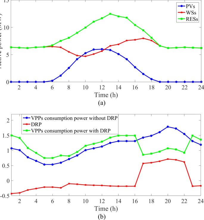
Expected daily curve of, (a) RESs, (b) consumption active power in all VPPs for β = 0.5.

Full size image

The projected daily curve of active power and reserve for VPPs is depicted in Fig. 6, derived from the DRP and RES performance curves. The total available capacity of VPPs is limited to 6.3 MW, preventing them from injecting additional active power into the ADN. The apparent power flowing through distribution lines, substations, and buses, along with bus voltage amplitudes, is constrained by ADN capacity and limitations. Under these conditions, excess power generated by the DRP and RESs is reserved in accordance with Eq. (13). Consequently, VPPs are exclusively accessible from 13:00 to 22:00, as illustrated in Fig. 6.

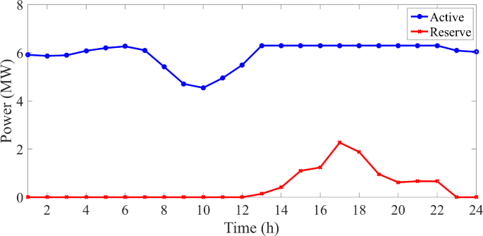
Expected daily active and reserve power curves of all VPPs for β = 0.5.

Full size image

Figure 7 presents the Profit-CVaR diagram for all VPPs for two case studies of a VPP with/without DRP. In this figure, β varies from 0 to 1 in steps of 0.1, where β = 0 (β = 1) corresponds to the left (right) side of the Profit-CVaR curve.

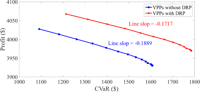
Curve of Profit-CVaR for all VPP for different cases.

Full size image

The diagram shows that an increase in α reduces the predicted profit of VPPs in the day-ahead energy and reserve markets while increasing the CVaR. The curve exhibits a minimal line slope and is nearly linear, indicating that profit fluctuations due to substantial CVaR changes are negligible. This suggests that VPPs can minimize low-profit risks by accepting a small reduction in profit. The Profit-CVaR curve for VPPs with DRP has a smaller slope (-0.1717) compared to those without DRP (-0.1889), as illustrated in Fig. 7. This demonstrates that, unlike VPPs without DRP, profit stability in VPPs with DRP is less affected by significant CVaR changes. The integration of DRP with RESs enhances the competitiveness of renewable producers in energy and reserve markets by effectively managing profit volatility within VPPs.

The anticipated profit of VPPs in DA energy and reserve markets for varying load levels and β = 0.5 is presented in Table 3. The table shows that the profit increases by approximately 1.4% to 1.7% (3.3% to 4.8%) when DRP is combined with RESs in the energy (reserve) market, compared to scenarios where RESs are the solitary participants. This indicates that the financial performance of these VPPs improves significantly, and DRP contributes positively to energy and reserve market operations. Additionally, the projected profit of VPPs decreases as the load level increases in these markets. At higher load levels, the DRP and RESs inject less power into the markets due to increased electricity generation within VPPs. However, Table 3 reveals that the profit gain in VPP case studies (with and without DRP) is directly proportional to the rise in load levels. This is because the profit derived from DRP increases with higher load levels, even though the profit from VPPs declines due to increased consumption.

Assessment of ADN operation status:

Table 4 presents the technical indices of the ADN, including operating cost (OC), VDF, expected energy loss (EEL), maximum voltage drop (MVD), and maximum overvoltage (MOV), for a 100% load level and β = 0.5. The indices are compared for two case studies: power flow studies (Case I) and the proposed scheme (Case II). As indicated in Table 4, the operating cost of the ADN is reduced from $8,507.2 in Case I to $4,153.2 in the proposed scheme (Case II), which incorporates optimal VPP management as described in Section “Results”. In other words, the quantity of OC is decreased by approximately 51.18% in comparison to power flow studies ((8507.4153–2.2)/8507.2). Additionally, the proposed strategy has significantly reduced the VDF, EEL, and MVD by approximately 51.95%, 41.25%, and 44.56%, respectively, compared to Case I. However, the data also reveal a 0.011 p.u. increase in MOV relative to Case I. Despite this increase, the MOV remains below the permissible limit of 0.1 p.u. (1.1 − 1).

This work presents a multi-objective operation of ADNs considering the participation of VPPs in day-ahead energy and reserve markets. VPPs serve as a system that simplifies the coordination of decentralized power planning with RESs. A bilevel optimization framework was integrated into the proposed architecture. Pareto optimization, regulated by AC-OPF equations and based on the weighted sum technique, was utilized to achieve optimal ADN operation. Upper-level problem minimizes operating cost of ADN and voltage deviation function. The lower-level problem addressed the risk model, constrained by operational models (DRP and RESs) and the reserve provided by the VPP. The single-level model was then derived using the KKT conditions, and the problem was solved using the SCA + TLBO hybrid procedure. Stochastic programming approach was employed to model the volatility of market prices, demand, and renewable energy generation. When compared to NHEAs, the numerical results demonstrated that the SCA + TLBO algorithm efficiently identified the optimal solution with the highest convergence rate. It consistently provided a final solution with a standard deviation of 0.95% across various load scenarios. In other words, it reliably delivers a nearly optimal solution, a characteristic rarely achieved by NHEAs. Moreover, when RESs operated independently in these markets, the combination of DRP with RESs within VPPs and the implementation of optimal power management resulted in significant financial improvements. Additionally, integrating DRP with RESs in the form of VPPs compared to operating RESs alone, enhances competitiveness and improves risk management regarding VPP profit volatility. In summary, compared to power flow studies, the optimal performance of ADNs resulted in significant improvements in operational indicators. These included reductions in operating costs (51.18%), energy losses (41.25%), and maximum voltage drop (44.56%). The proposed scheme considered only a single model of DRP. However, DRP encompasses various models, each of which can have specific impacts on the technical and economic performance of the network. Future research should focus on analyzing the effects of different DRP models within the proposed design framework.