Conditional variational auto encoder based dynamic motion for multitask imitation learning

Introduction
Manipulation is a fundamental skill for robots operating in diverse domains, including manufacturing1,2, healthcare3,4,5, and domestic environments6. As robots become more advanced7, learning new skills is crucial to handle complex tasks autonomously. One of the most effective approaches to acquiring skills in robotics is Learning from Demonstration (LfD)8,9. By observing and imitating a human’s or another agent’s actions, the robot can learn to generate the desired behaviors. There are two main challenges in learning from demonstrations. First, a large number of demonstrations: The robot needs to obtain enough demonstrations to learn the desired behavior precisely. Second, generalization of the learned behavior: The robot must adapt the learned behavior to unseen situations in the task.

Mulit-task imitation learning. Different tasks have distinct trajectory shapes. The trajectory for the reaching task looks like a straight line, while the trajectory for the pushing task takes an L shape, and for grasping, it resembles a U shape. Images were generated using PyBullet (version 3.2.5 available at http://pybullet.org).
Among various LfD techniques, Dynamic Motion Primitive(DMP)10 based methods have achieved great success in the above-stated challenges. Dynamic Motion Primitive (DMP) is a framework that uses dynamic systems to control goal-directed robotic movements by representing desired states as attractors. This method can generate smooth, adaptive, and flexible motions in dynamic environments. Unlike exploration-based methods, such as deep reinforcement learning11,12, DMP-based methods require less training data and time. They enable the direct extraction of global task-related information from complete trajectories rather than learning from trial and error. Furthermore, unlike basic imitation learning techniques, such as behavior cloning13, which simply replicates expert behavior through supervised learning, DMP-based methods can be conditioned on task parameters and adapted to new situations based on those parameters14.
Currently, most of the motion primitive methods focus on a single task. For instance, in the work of Ijspeert et al.10, a second-order dynamic system is used to generate the desired trajectories. By defining primitive forces, complex trajectories can be generated by combining these forces with different weights. However, this method is designed to learn from one demonstration and does not consider the relationships between different degrees of freedom (DOF) in the demonstration. Paraschos et al.15 were the first to use a probabilistic model to learn motion primitives from multiple demonstrations. More recent works by Felix Frank et al.16 and Michael Przystupa et al.17 address constraints and higher dimensions of the observation space.
In this study, we propose a variational auto-encoder(VAE) based dynamic motion technique to learn multi-task at the same time. Inspired by the works of DMP10 and VAE18. Our method consists of two stages: training stage and generation stage. During the training stage, we collected several normalized demonstrations for different tasks. The desired force is derived from an inverse dynamic system using these demonstrations. Then, a conditional variational auto-encoder (cVAE) model is trained to learn the distribution of the different forces. In the generation stage, a force is sampled from the Decoder model based on the corresponding task class. This force is then input into the dynamic system to generate a normalized trajectory. We define an error between the normalized trajectory and the via-point (including the endpoint). Finally, the decoder and scaler parameters are updated to minimize this error.
The main contributions of our work are given below:
-
Multi-task learning in a single module with one demonstration per task: We propose a cVAE-based method that learns multiple tasks simultaneously, using only one demonstration for each task.
-
High-precision trajectory generation: Our method takes advantage of dynamic motion and cVAE. The generated trajectory satisfied the initial and final state automatically with the help of a dynamic motion system.
-
Efficient trajectory generation: The trajectory can be adjusted to new task conditions within 0.5 seconds, and the decoder and scaler parameters can be fine-tuned within 1 second.
Related work
Deep learning-based learning from demonstration methods, such as Deep Reinforcement Learning (DRL), Offline Reinforcement Learning (ORL), and various imitation learning frameworks, have achieved significant success in robotic manipulation tasks. For example, Gu et al.19 developed an off-policy deep Q-learning approach for robotic manipulation. However, training a deep reinforcement learning-based agent typically requires millions of interaction steps with the environment. Learning from demonstrations is a viable alternative to avoid long and uncontrollable interaction phases. By collecting successful trajectories, imitation learning methods like behavior cloning can be applied. Chen et al.20 introduced a conditional diffusion model within the behavior cloning framework, achieving a high success rate (near 100%) in robotic manipulation tasks such as pushing and peg-in-hole. Nevertheless, most deep learning-based demonstration methods typically require hundreds to thousands of successful trajectories, making it time-consuming to create such datasets and limiting their applicability to new, unseen tasks. In this paper, we propose a lightweight deep-learning framework that can learn from demonstrations using only one or a few trajectories from scratch.
Traditional DMP-based methods10 were designed to learn from a single trajectory for a single task, but they cannot handle multiple trajectories for multiple tasks. Probabilistic Movement Primitives (ProMPs)21 were proposed to learn multiple trajectories for a single task using a linear Gaussian model. However, this method is still limited to learning only one task, as Gaussian-linear models are restricted to unimodal distributions. To address this limitation, more recent work22 explored a deep network-based Gaussian mixture model with a Bayesian Aggregator, which shares the same structure and training process as cVAE. However, this approach still requires thousands of demonstrations for training.
Methods that combine DMP and cVAE can be categorized based on whether the cVAE works as an encoder or a generator. When the VAE acts as an encoder, DMP is trained in the low-dimensional latent space encoded by the VAE, as seen in the work of Chen et al.23,24. Conversely, when the VAE functions as a generative model, Przystupa et al.17 use via-points and context information (describing features of the environment) as inputs to the VAE. New trajectories are then generated by sampling from the latent variables of the VAE. A similar approach to our work was proposed by Noseworthy et al.25, where DMP creates a dataset with varying task conditions. The cVAE module is then trained and conditioned on these task parameters. Additionally, they introduced an Adversarially Enforcing Independence (AEI) method to disentangle the latent space from task parameters, reducing generalization errors for new tasks. However, their work primarily focuses on a single task, and because they use a deep neural network-based cVAE, generalization errors persist with untrained data.
In this work, we combine the advantages of cVAE and DMP. The cVAE generates diverse types of trajectories, while the DMP ensures high precision and convergence to the goal state. We use the cVAE model to create a virtual torque that shapes the trajectory, and the DMP model generates the final trajectory based on this virtual torque, ensuring an accurate endpoint position.
Problem formulation
Priliminiries
This section will provide a brief introduction about the essential background of dynamic motion primitive and conditional variational auto-encoder.
Dynamic motion primitive
Dynamic Motion Primitive (DMP) is a method used to generate desired trajectories using a second-order dynamic system. This approach ensures both scalability and convergence of the trajectory toward the goal state. The dynamic system can be defined as:
where, y is the state in the trajectory, g is the goal state, (tau) is the time scale, (alpha) and (beta) are the parameters of the dynamic system, f is the force term. This dynamic system defines the goal state as an attractor, guaranteeing the trajectory convergence to the goal state. The force f is calculated as a weighted sum of the Gaussian basis functions. As shown in the work of Ijspeert et al.10, the force term can be calculated as in Eq. 2.
where, (w_i) is the weight of the ith Gaussian basis function, (psi _i(t)) represents the ith Gaussian basis function, t is the time factor decrease from 1 to 0, (y_0) is the initial state of the trajectory.
Equation 2 describes how the desired control force is proportional to the error term. This error term represents the difference between the current and designated goal states. Consequently, the trajectories toward new goals are achieved by scaling the force term based on the desired final state.
Conditional variational auto-encoder
Variational Auto-encoder(VAE) is a generative model that can learn the distribution of the data set in the latent space. Conditional Variational Auto-encoder(cVAE) is a variant of VAE. The cVAE model is trained by maximizing the evidence lower bound (ELBO) of the dataset conditioned on task parameters. The ELBO of cVAE can be defined as:
where, c is the task parameters, (theta), and (phi) are the parameters of the decoder and encoder, x is the input data. z is the latent variable, (q_phi (z|x, c)) represents the encoder, whereas (p_theta (x|z, c)) represents the decoder, the term p(z|c) is the prior distribution of the latent variable conditioned on the task parameters.
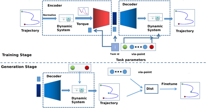
The figure illustrates the two main stages of our method: Training Stage: The Conditional Variational Autoencoder (cVAE) structure is optimized based on the task ID and via points. The encoder and decoder comprise a second-order dynamic system and a deep neural network. Generation Stage: A new trajectory is generated by first sampling a torque from the latent space using task parameters. Then, the trajectory is produced by the dynamic system in the decoder based on the sampled torque.
cVAE has been widely used in computer vision as a generative model to create images. Inspired by the work of Doersch et al.26, the cVAE model is trained on the Mnist dataset27, where numbers are generated in pixels. In robotic applications, different tasks usually have different shapes of trajectories. For example, the reaching task has a trajectory that looks like a straight line, while the trajectory of the grasping task looks like a ({{textbf {U}}}) shape. The robot goes to the object’s position and then lifts it to a certain height. A straightforward approach is to generate different trajectory shapes by conditioning on the types of tasks.
Problem modeling
In this section, we address the problem of multi-task imitation learning using a cVAE-based DMP from demonstrations. The demonstration dataset (D) consists of (m) types of tasks, with each task having (n) trajectories represented as (T). The dataset D can be defined as:
where, (D_i) is the ith task, (T_k) is the kth trajectory of the ith task.
Each trajectory in (T) consists of (L) state points, each of which is (d)-dimensional. Additionally, the trajectory incorporates user-defined task parameters, including the task ID and via-points. The trajectories can be defined as:
where (x_l in {mathbb {R}}^d) is the (l_{th}) state point of the trajectory, i is the task id, and C is the set of the via-points.
Our method aims to learn a trajectory generator (G) from the dataset (D). (G) can generate new desired trajectories given the relevant task parameters.
Proposed approach
This section provides details of our proposed cVAE-based DMP approach. The main process of the proposed approach is shown in Fig. 2. The proposed method consists of two stages: the training stage and the generating stage. During the training stage, we focus primarily on the trajectory’s initial point, endpoint, and overall shape. The model consists of two main components: an encoder and a decoder. Each component incorporates a second-order dynamic system and a deep neural network. In the encoder, trajectories are normalized to the range from 0 to 1. These normalized trajectories are then input into the dynamic system to obtain the desired force, with a 1D-CNN-based deep neural network used for further processing. In the decoder, the desired force is sampled from the latent space of the cVAE. This force is then scaled according to the error between the initial and final states. Finally, the dynamic system generates the reconstructed trajectory.
During the generation stage, the decoder module generates a trajectory based on the task ID, initial state, and goal state. The decoder’s parameters can be fine-tuned according to the distance between the generated trajectory and the via-points. Below, we provide the details of the data augmentation, training stage, and generation stage. To better illustrate the developed approach, we use the number handwriting dataset to demonstrate the process.
Date augmentation
Training the deep cVAE module requires a large amount of data. However, building such a large dataset from human demonstrations is time-consuming. To address this issue, we use data augmentation to generate new data.
Given a demonstration, we first normalize it to the range from 0 to 1. The desired torque is then calculated using Eq. 2. Once the torque is obtained, Gaussian noise is added to the weight of each Gaussian basis function, as shown in Eq. 6. This process yields a set of forces, illustrated in Fig. 3b. Finally, these forces are input into the dynamic system defined by Eq. 1 to generate a new trajectory, as shown in Fig. 3a. The blue line represents the original trajectory, while the colored lines depict the new trajectories generated through data augmentation. For the handwritten digit number problem and robotic manipulation tasks, we create a small dataset by performing data augmentation 10,000 times for each trajectory.
where: f is the virtual force that generates the desired trajectory. (gamma) is the scale factor. (epsilon) is the Gaussian noise.
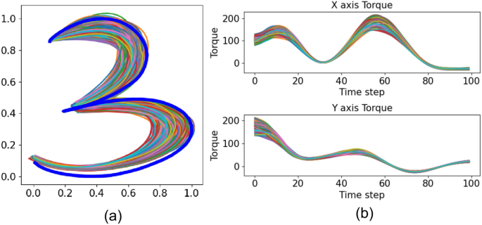
Data augmentation. (a) Augmented trajectory. The blue line represents the original trajectory, and the colored lines are the trajectories generated using data augmentation. (b) Augmented torque by random adds noise in the weights of the Gaussian base function.
Training DMP based cVAE
In this work, we use a DMP-based cVAE model to learn and reconstruct the distribution of the latent space of the trajectories. Specifically, the modified deep cVAE model consists of an encoder and a decoder. The encoder includes a dynamic system (Dy) and a force encoder (En), which is composed of 1D-CNN and fully connected layers. The decoder consists of a deep neural network based force decoder (De) and a dynamic system (Dy)
Given a trajectory (T_k), we obtain the force (F) by the inverse dynamic system: (F = Dy^{-1}(T_k)). The force encoder calculates the latent variable (z) as (z = En(z|F, i)), where (i) is the task ID. This structure builds upon the work of Doersch26, which employs a 2D CNN as the encoder. We modify their network using 1D CNN and fully connected layers in our work. For the number handwriting task, (i) ranges from 0 to 9.
In the decoder module, a force decoder is trained to reconstruct the force (F’) by the deep neural network from the latent variable (z), where (F’ = De(F|Z, i)). Finally, the reconstructed trajectory is obtained by the dynamic system: (T’ = Dy(F’s|x_0, g)), where (x_0) is the initial state of the trajectory and (g) is the goal state defined in Eq. 1. (s) is the scale parameter of the force term. The loss function for the training stage can be defined as follows.
where: (T_k) is the kth trajectory in the data set D, K is the total number of trajectories. (x_0) and g are the initial state and goal state of the trajectory. s is the scale parameter of the force term that needs to be optimized. p(z|i) is the prior distribution of the latten variable z, which usually selected as standard Gaussian distribution.
Since the dynamic system is deterministic and known, Eq. 7 can be solved in an engineering manner. Instead of training the encoder and decoder at the trajectory level, we first train the cVAE at the torque level by optimizing the evidence lower bound of (F) and (F’) using Eq. 3, and then update the scale parameters (s) using Eq. 8.
where (s_0) is the initial value of the scale parameter, (g_i) is the goal state of the ith trajectory, (x_i^{end}) and (x_i^{0}) are the end state and the initial state of the (i_{th}) trajectory.
Trajectory generation stage
Our generation stage consists of two steps: (1) initial trajectory generation and (2) fine-tuning the trajectory based on via-point constraints. Given an unseen case in the trained task, we first generate a trajectory that satisfies the initial state and final state, and we shape the requirements of the task based on the start state, end state, and task ID. Then, the decoder parameters are fine-tuned to meet the via-point constraints. The entire process is illustrated in the generation stage in Fig. 2. Below, we provide details about the two-step generation process.
Initial trajectory generation
The initial trajectory is generated by fist sampling the latent variable (z) from the latent space. Then, the force (F) is then produced by the force decoder (De) using the sampled (z) and task ID (i). This force is input into the dynamic system via Eq. 1 to generate a normalized trajectory (T). Finally, the initial trajectory is created by scaling the normalized trajectory using the scale parameter (s) in Eq. 8 to satisfy the end-point constraint.
As shown in Fig. 4, we can generate trajectories with different shapes that satisfy the initial and final state constraints. In Fig. 4a, the trajectories begin at point ([0, 1]) and end at point ([0.5, 1]). These trajectories are generated using task IDs 1, 3, and 7, each following a distinct shape as they move from the starting point to the endpoint.
Since the dynamic system generates the trajectories, our model inherits the scalability of DMP. In Fig. 4b, we demonstrate this capability. We generate three trajectories with the same task ID, number 3. The trajectories begin at point ([0, 1]) and end at three different points (a) ([0.3, 0]), (b) ([0.5, 0.5]), and (c) ([0.8, 0]). Once the torque decoder module generates the torque, we simply scale the torque using Eq. 8 to reach the desired goal state.
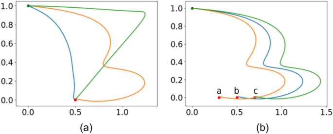
Trajectory Generation for different tasks and endpoints. (a), all the trajectories begin at [0, 1], and end at [1, 0]. (b), trajectory ends at different points.
Via point constrain
To complete a task, the trajectory must not only satisfy the initial and final states but also pass through the required via points. For example, in a robotic grasping task, the manipulator must first reach the object’s position, then grasp it, and finally move it to a specified height.
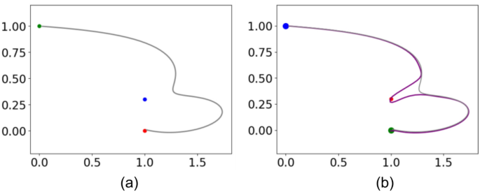
Finetune for via point constrain. (a) is the initial trajectory. (b) is the trajectory with via point constrain.
The decoder parameters are optimized to satisfy the via-point constraints by minimizing the loss function defined in Eq. 9. This loss function consists of three components. The first component penalizes deviations from the original trajectory, ensuring the overall shape is preserved. The second component constrains endpoint displacement in the new trajectory, and the third minimizes the distance between the regenerated trajectory and the specified via points.
where: (L) is the length of the trajectory, (C) is the number of via points, (T) is the initial trajectory, and (T’) is the trajectory generated after fine-tuning. (x_i) represents the (i)th point in the trajectory (T), and (g) is the goal state of the new task. The term (text {dist}(T’, C_k)) denotes the minimal distance between the via-point and the trajectory.
The force decoder (De) consists of three fully connected layers. In this task, we found that freezing the parameters of the first two layers yields the best fine-tuning results. Figure 5a shows the initial trajectory for drawing the number 3, generated by the force decoder module. The blue point represents the required via point. The fine-tuned trajectory, shown by the red line in Fig. 5b, successfully passes through the via-point while maintaining a shape similar to the initial trajectory.
Experiment
We use handwriting and robot manipulation tasks-such as reaching, pushing, and grasping-to demonstrate the effectiveness of our method. To evaluate our approach systematically, we use the following metrics:
-
Via-point error The minimal distance between the via-point and the trajectory.
-
Final state error The distance between the goal state and the endpoint of the trajectory.
-
Success rate/Trajectory shape For robotic manipulation tasks in the PyBullet environment, this metric represents the success rate of the task. For the handwriting task, which lacks a specific success state definition, we compare the shape of the desired trajectory with the generated trajectory.
For data augmentation, we select 50 Gaussian basis functions in Eq. 6. The force encoder consists of four convolutional layers with channel sizes ([16, 32, 64, 64]), each followed by batch normalization and ReLU, along with two max-pooling layers. Afterward, a flattening operation is applied, followed by an MLP with a single hidden layer (16 units). The condition information is compressed into 8 channels. The force decoder is an MLP with layer sizes [24, 64, 128, 200], followed by a Sigmoid activation.
Number handwriting
In this paper, we do not consider rhythmic movements which have the same start and end state. The numbers 1, 2, 3, 6, and 7 are selected for the handwriting dataset, as numbers 0, 4, 5, and 8 require multiple strokes or have identical start and end points. Additionally, since 6 and 9 have similar shapes, we include only 6 in the experiment.
The original data set and the one with data augmentation are shown in Fig. 6.
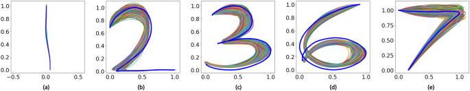
Data augmentation for four tasks. Figures (a) to (d) show the number writing tasks 1, 2, 3, 6, and 7, respectively. The blue line represents the original trajectory, while the colored lines depict the trajectories generated through data augmentation.
Final state error
Here, we test our method’s ability to converge to unseen endpoints. For each task, the trajectory begins at ([0, 1]) and ends at a point ([1, 0] + 0.3 cdot r), where (r) is standard Gaussian noise. The final state and the demonstration endpoint for each task are shown in Fig. 7 as green and red points, respectively. We randomly selected 50 endpoints for each task, represented by blue points. The training time of our method is approximately 12 seconds per task. The final state error for each task is shown in Table 1. Initially, the trajectory error is below 0.02 for the normalized trajectory, and after fine-tuning, the final state error is reduced to below 0.008. Among the tasks, task 1“writing the number 1”has the lowest error, likely due to the simplicity of its trajectory.
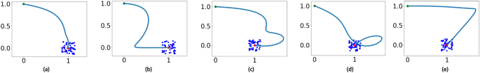
Test error for different endpoints. The blue points represent randomly generated endpoints for each task, used to test the convergence of our methods to the desired endpoints.
Via-point error
In this section, we test the adjustability of our method with unseen via-points. For each task, the via-point is selected by offsetting the midpoint of the trajectory by -0.2 along the x-axis. Figure 8 shows that our method can adjust the trajectory to the new via-point while preserving its overall shape. The retraining time for fine-tuning each task is approximately 2.2 seconds. In this test, the via-point offset is 20% of the trajectory range, which is unusually large for most robotic tasks and results unnature looking trajectories. This method can work well for typical robotic applications where via-point adjustments are small. For instance, in pushing or grasping tasks, a 5 cm via-point offset represents only 5% of a 1 m trajectory, causing minimal distortion, as shown in the trajectories in Fig. 17. As seen in Table 1, the via-point error is below 0.005 for each task. This indicates that if the robot’s workspace is around 1 meter, the via-point error is less than 5 mm, which is acceptable for most robotic tasks.
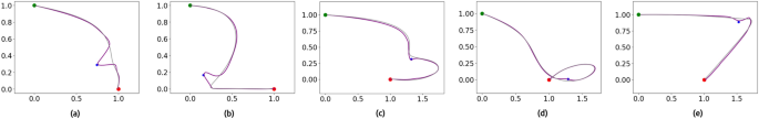
Test error for the via-point. The red trajectory is after fine-tuning, and the blue point is the via-point. The fine-tuned trajectory passes through the via-point.
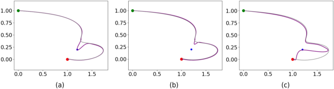
Different finetune paramter. (a) fine-tuned. (p_1 = 0.6, p_2 = 0.2, p_3 = 0.2). (b) Not tuned. (p_1 = 0.9, p_2 = 0.05, p_3 = 0.05). (c) Over tuned. (p_1 = 0.05, p_2 = 0.05, p_3 = 0.9).
Trajectory shape
We also evaluated the shape of the generated trajectory. According to Eq. 9, there are three conflicting terms: The first term, (p_1), aims to keep the newly generated trajectory’s shape close to the initial trajectory. The second term, (p_2), limits the endpoint offset in the new trajectory. The final term, (p_3), minimizes the distance between the via-points and the new trajectory. When these parameters are set properly, the trajectory will pass through the via-point while maintaining its original shape, as shown in Fig. 9a. If (p_1) is too large, the new trajectory may fail to blend with the via-point, as shown in Fig. 9b. Conversely, if (p_3) is too large, the trajectory may overly conform to the via-point, as seen in Fig. 9c, which can alter the trajectory’s shape. In this study, we set (p_1 = 0.6), (p_2 = 0.2), and (p_3 = 0.2), balancing via-point tuning and shape preservation. As shown in Table 1, the shape error of the trajectory is less than 0.015.
Conclusion and compared with classic methods
In this subsection, we compare our proposed methods with the classic DMP and cVAE in terms of data requirements, precision, training time, over-scaling, and performance on out-of-demonstration (OOD) in the number writing data, as summarized in Table 2.
Both DMP and our proposed methods require only one demonstration per task. DMP and our methods achieve high precision at the endpoint, with average errors of 0.0271 and 0.0159, respectively, across the five tasks. After fine-tuning, the endpoint error of our methods is further reduced to 0.0053. Although the classic DMP method can be trained within 0.01 seconds, it cannot handle multiple tasks. Our proposed method can also be trained in an acceptable time (65.438 seconds), similar to the training time of deep neural network-based cVAE methods, as they share the same network structure.
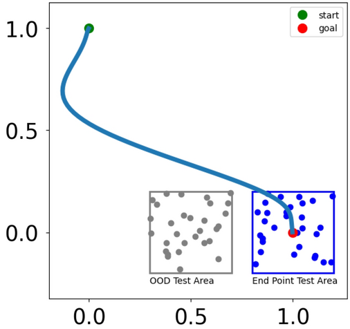
Training and Out-of-Demonstration (OOD) Test End Points. The blue square represents the region from which end points are sampled for training and testing, centered at [1, 0] with a range of 0.2. The gray square indicates the region used to evaluate OOD performance.
For the cVAE, we created two custom datasets containing 200 and 2000 demonstrations per task, for numbers 1, 2, 3, 6, and 7. The trajectories start at the position ([1, 0]) and end near ([1, 0]) with added noise, as illustrated by the blue square in Fig. 10. The noise is sampled from a uniform distribution ranging from (-0.2) to (0.2). From Fig. 11, the basic cVAE requires thousands of demonstrations to generate smooth trajectories. With only 200 demonstrations, the cVAE fails to produce smooth trajectories. Even with 2000 demonstrations, while the cVAE generates trajectories with the correct shape, it struggles to satisfy the endpoint constraint, resulting in an average error of 0.1748 across the tasks. Notably, our method demonstrates robust performance even on OOD test cases, achieving an error of 0.0161 without fine-tuning. The OOD test area, centered at the point ([0.5, 0],) with random noise sampled from a uniform distribution ranging from (-0.2) to (0.2), is shown as the gray area in Fig. 10.
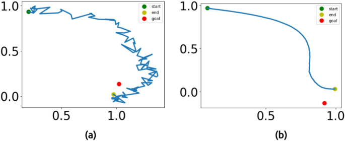
Performance of cVAE. (a) Trajectory generated for number 1 using 200 demonstrations. (b) Trajectory generated for number 1 using 2000 demonstrations.
A significant limitation of the basic DMP is its tendency to over-scale when the endpoint is close to the starting point. As depicted in Fig. 12, for task 7, where the starting and ending x-values are near, the trajectory is unnecessarily distorted in the x-direction. Our proposed method effectively addresses this issue, as evidenced by the orange line in Fig. 12.
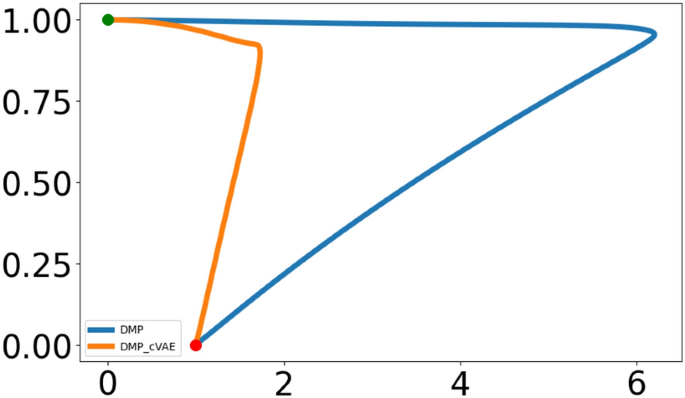
Over-Scaling in basic DMP. The blue line shows the basic DMP trajectory, while the orange line shows our cVAE-DMP trajectory.
Additionally, our framework simplifies the via-point problem by fine-tuning the deep neural network responsible for torque generation. In contrast, the basic DMP method requires trajectory segmentation at the via-point, which can lead to less smooth trajectories. Other approaches, such as probabilistic DMP, are only effective when the via-point is not too far from the trajectory and often require multiple demonstrations28.
Robotic task
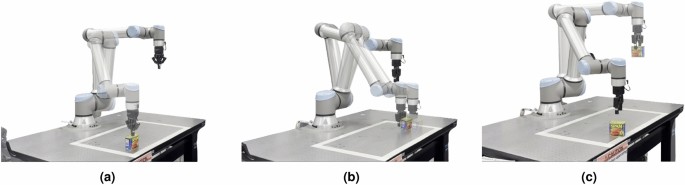
We applied our method on three types of robotic manipulation tasks: reaching, pushing, and grasping, as shown in the Fig. 13.
-
Reaching Task: As shown in Fig. 13a, the goal is to touch the can with the UR10 gripper. In this task, there is no via-point constraint.
-
Pushing Task: As described in Fig. 13b, this task aims to push the can into a desired position. There is one via-point constraint in this task: the robot manipulator must first move to a position behind the can before pushing it.
-
Picking Task: The entire process of this task is illustrated in Fig. 13c. The robot’s gripper needs to reach the can and then grasp it. This task involves one via-point constraint: the robot must first reach a point above the can with the gripper open.
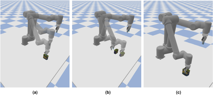
Reaching, Pushing and Grasping task in the pybullet simulation environment. Images were generated using PyBullet (version: 3.2.5 available at http://pybullet.org).
We tested our proposed method in a PyBullet29 simulated environment using a UR10 robotic manipulator and applied the trained network to a similar real-world setting. As illustrated in Fig. 14, our method follows three main steps, similar to the handwritten digit generation task: (1) Collect demonstrations, (2) Train the cVAE-DMP network, and 3) Generate the trajectory for the new goal state.
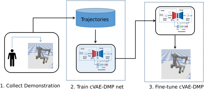
Steps to apply our methods on robotic manipulation task. 1. Collect demonstration with a joystick. 2. Train the cVAE-DMP with the collected trajectories. 3. Generate trajectories for new goal states and fine-tune them in the case of failure. Manipulator images were generated using PyBullet (version: 3.2.5 available at http://pybullet.org). The overall figure was created using PowerPoint, available at https://www.microsoft.com/en-us/microsoft-365/powerpoint.
Collect manipulation demonstration
We use a Logitech 3D Pro joystick to control the robot and capture trajectories within the simulation environment. A single demonstration is collected for each task, as shown in Fig. 15.
Figure 15a shows the reaching process, during which the robotic gripper remains closed. The collected trajectory is not linear. Due to the simulation environment’s limitations in rendering depth realistically, we must adjust the trajectory throughout the reaching process. For the pushing task, as shown in Fig. 15b, the robot’s gripper remains at a fixed width throughout the process. The trajectory shape looks like an “L”. Finally, for the grasping task, the robot first reaches above the can and then closes the gripper to grasp both sides of the object.
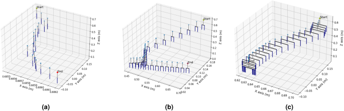
Collectted demonstration for three robotic tasks. (a) Reaching trajectory. (b) Pushing trajectory. (c) Grasping trajectory.
Train cVAE-DMP network
Since there is a deep neural network part(cVAE) in our proposed cVAE-DMP methods, a number of different data are needed to train the cVAE. To avoid the tedious data collection process, similar to the digital number writing task, we do data augmentation at the force level by Eq. 6. 10000 are generated for each manipulation task. The scaling factor k equals 0.3 in Eq. 6.
Figure 16 shows the ten torque samples after date augmentation with Eq. 6. It can be observed that the torque begins from different values but ends with the same values for all the tasks. The shape of the torque is similar to the shape of the robotic manipulator trajectory, where the reaching task has a “c” shape, the pushing task has an “L” shape, and the grasping task looks like a “C” shape. Compared to the collected initial trajectory, as shown in Fig. 15, the torque generated with DMP is smoother, as this torque is approximated with some basic Gaussian function. It takes around 30 seconds to train our proposed cVAE-DMP models in 200 epochs on a laptop with a 4060 GPU, 13th Gen i9 Intel.
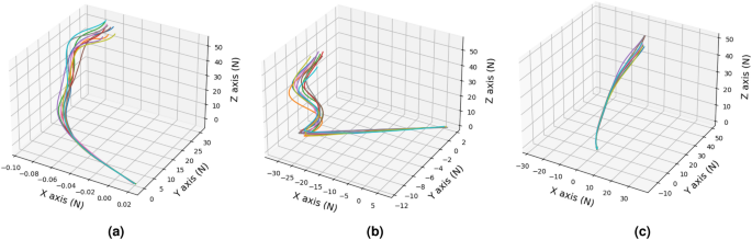
Data augmentation at torque level. (a) Torque for reaching task. (b) Torque for pushing task. (c) Torque for grasping task.
Test on the unseen situation
Our method leverages DMP advantages to handle new tasks effectively. It takes about 0.5 seconds to generate the desired trajectory based on the task ID and endpoint constraints.
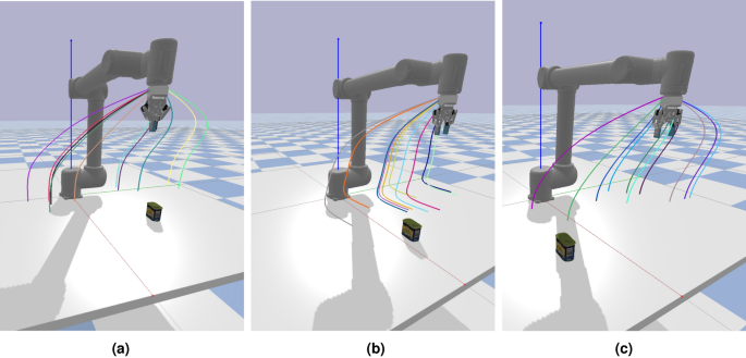
Test on unseen situation. (a) Reaching task. (b) Pushing task. (c) Grasping task. Images were generated using PyBullet (version: 3.2.5 available at http://pybullet.org).
-
Reaching Test: In this test, the robot’s objective is to touch the upper surface of the can with the gripper. The task is considered a success if there is no displacement of the can, distortion of the can’s surface, and deformation of the gripper fingers, as these indicate a collision between the gripper and the can. The can was placed randomly on the table within an x-range of 0.3m to 0.8m and a y-range of -0.45m to 0.45m. As shown in Fig. 17a, we sampled 10 different end positions for the robot to reach. Our proposed method successfully generated accurate reaching trajectories in all instances. Notably, the cVAE-DMP method achieved a 100% success rate in this task without requiring any fine-tuning.
-
Pushing Task: As for the pushing task, similar to the demonstration, the robotic manipulator will push the can along with the x-axis for 0.12m. If the final position of the can box deviates from the desired position by less than 0.05 cm and the box does not fall during the pushing process, the pushing task is considered successful. We randomly put the can on the table with x range from 0.5m to 0.7m, ensuring no rotation along the z-axis. As shown in Fig. 17b, the cVAE-DMP model successfully generated the correct pushing trajectory, even when the can was positioned at different locations. Our method achieved a success rate of 96.7%, with only one failure case. The failure can be addressed by defining a via-point positioned 0.1m behind the can, while keeping the gripper open by 0.56% and maintaining a zero-degree rotation angle.
-
Grasping Task: We further evaluated our method on the grasping task, where the gripper’s fingers are required to hold the can. The trajectory for this task is similar to the reaching task but with the added complexity. The gripper must first position itself above the can before descending to grasp it and then closing the gripper. The position and orientation of the meat can are randomized. To be considered a successful case, both grippers must contact the can, lift it at least 5 cm above the table, and hold it for more than 15 seconds. Figure 17c illustrates the trajectory of the grasping task, while Fig. 18 depicts the gripper’s state and its rotation along the z-axis. These figures show that the gripper consistently performed the same during the grasping process, even when the can was placed in different positions. Additionally, our method matched the rotation requirements, allowing the gripper to adjust its orientation within 40 steps. The approach demonstrated a success rate of 93.3%, with two failures. These failures could be rectified by defining a via-point 2cm above the can while keeping the gripper open during the approach.
Apply to the real robot
Finally, we transferred our method directly to a real robot for validation. a UR10 robot is used to perform all manipulation tasks. A meat can from the YCB dataset was randomly placed in the workspace, marked by a white square on the table in Fig. 19. We utilized a ROS (Robot Operating System)-based framework to control the UR10 robot. The position and orientation of the meat can were localized by moving the gripper to the desired location on the table, after which the can placed. The object placement mirrored the random positioning used in the simulation environment, allowing us to seamlessly transfer the trajectories generated in the simulation to the real-world scenario .
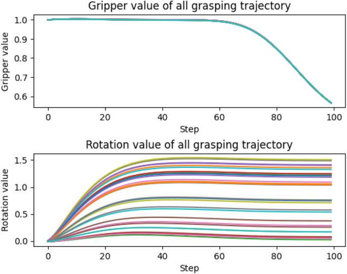
Gipper value and rotation value during the grasping process. 1. Gripper value of 10 grasping trajectory. 2. The rotation value of 10 grasping trajectories.
Test on real environment. (a) Reaching task. (b) Pushing task. (c) Grasping task. These real experiments were captured in the lab and combined using PowerPoint, available at https://www.microsoft.com/en-us/microsoft-365/powerpoint.
Figure 19 shows that the simulated trajectories were effective in all three real-world tasks. As illustrated in Fig. 19a, the reaching task is considered successful if the robot touches the can. For the pushing task (Fig. 19b), the goal is to push the can along the x-axis by 12 cm. The grasping task requires the robot to grasp and hold the object while returning to its home position, as shown in Fig. 19c.
Our proposed approach achieves a 100% success rate in the reaching task and a 93.33% success rate in both the pushing and grasping tasks. In contrast to traditional data-intensive deep learning methods, this high level of performance is accomplished with only one demonstration per task, showing the efficiency and effectiveness of our method in managing tasks with minimal data.
Conclusions and future work
In this paper, we propose a cVAE-based DMP method that inherits the flexibility of the deep cVAE, and the scalability property of DMP. It can learn to generate trajectories for multiple tasks within a single module while overcoming the over-scaling issue of basic DMP. Similar to DMP, it can adapt to different goal states. The effectiveness of this method has varied on the handwriting data set and robotic manipulation task – reaching, grasping and pushing. However, like the typical DMP based method, the main drawback of our method is that via-point and end-point(or end state) have to be defined by the user based on the understanding of the task. In addition, the correct trajectory type has to be selected by ourselves based on our previous experiment. In the later work, we could combine our method with the large language models (LLM). Therefore, LLM can work in a high-level way by defining the task ID, via-point, and end-point. Our cVAE-DMP can generate a precise trajectory based on this information.
Responses