3D magnetotelluric imaging of a transcrustal magma system beneath the Campi Flegrei caldera, southern Italy

Introduction
Caldera volcanoes constitute a significant natural hazard, having produced the largest volcanic eruptions on Earth (>1000 km3 of magma)1. The low frequency and high magnitude of the eruptions2, coupled with limited information regarding the physical dynamics and architecture of crustal magma systems beneath these volcanoes, severely impairs our understanding of where in the crust melts are stored and their ascent pathways3,4,5, which are crucial information for effective monitoring and hazard mitigation. Many questions remain unresolved regarding the magmatic systems that produce caldera-forming eruptions, particularly with respect to: the dynamics of deep (lower crustal) magma storage regions, the amount of eruptible magma that can be stored in the crust (and its lifetime), the transfer mechanisms and structures that extend into the shallower crust, and the processes that proceed high-magnitude and caldera-forming eruptions. Understanding the physical structure of the sub-volcanic system which underlies these structures is central to resolving these issues. In this regard, the concept of “magma chambers” has remained central to conceptual models of volcanic eruptions for several decades, especially from a hazards viewpoint, and is a common starting point for interpreting signals of unrest6. This is supported by geological evidence (e.g. layered intrusions) which attest to the presence of large melt-rich crustal magma bodies7. However, in response to new geophysical and petrological datasets, our conceptual understanding of magmatic systems has begun to shift8. There is an emerging consensus within the volcanological community that magma storage and differentiation occur at different depths, often within bodies throughout the crust, characterized by a combination of melt-dominated lenses and crystal-rich mush zones that are periodically reactivated and remobilized by the arrival of hot magma batches from depth5,8,9,10,11,12,13,14 or by fractional crystallization and oversaturation of volatiles in shallow magma reservoirs15. Such complex plumbing systems are particularly common beneath large volcanic centres or caldera systems, where volcanism has been active over a prolonged time period, repeatedly producing high-magnitude eruptions16. Envisioning magmatic systems as being in a mush-dominated state has enormous consequences for crustal magma dynamics, the architecture of the plumbing system and deep fluid circulation, and our understanding of eruption triggering mechanisms.
Geophysical characterization is crucial for advancing our understanding of the structure of magmatic systems, and has been instrumental in understanding the plumbing systems beneath several large volcanoes17. The magnetotelluric (MT) method is particularly well-suited for volcanic areas due to its ability to image resistivity contrasts associated with key geological features, such as magma chambers, hydrothermal systems, and fluid pathways. This capability stems from the method’s sensitivity to variations in electrical conductivity caused by changes in temperature, fluid content, and rock composition, making it a powerful tool for understanding subsurface processes in active volcanic systems. Consequently, MT provides valuable insights, elucidating the distribution of melt and hydrous fluids in the subsurface18 and tectonic structures, which can accommodate magma storage and facilitate the migration of crustal melts and fluids to surface19,20.
An important caldera system which urgently requires information about its subsurface structure is Campi Flegrei, Italy. This volcano has produced explosive eruptions21 which vary considerably in magntitude, with the most recent eruptions in the range M4-5 (0.1-1 km3 of dense rock equivalent magma; DRE)22 spanning up to the 40 ka Campanian Ignimbrite eruption23 with a magnitude of M7.8 ( ~ 250 km3 DRE of magma ejected). While trans-crustal24 and crystal mush-dominated magmas have been identified beneath Campi Flegrei prior to very large caldera forming eruptions25, it remains unclear whether a similar architecture exists today. Information regarding the structure of the Campi Flegrei magmatic system is critically lacking due to difficulties in carrying out broad geophysical surveys as the caldera is heavily developed and densely populated, and a large portion lies underwater. Understanding the magmatic architecture and the amount of magma beneath the volcano is essential for accurately assessing the current volcanic risk and interpreting monitoring data; for example, developing a monitoring scheme that could result more based than the simple idea of localized melt storage confined in defined part of the subsoil. Campi Flegrei is one of the most active caldera systems on Earth and is currently exhibiting significant unrest within an area inhabited by >500,000 people; recent increases in seismicity have led to precautionary evacuation of the local population. Here, we present a new MT survey of the Campi Flegrei region, which provides a 3D resistivity model of the sub-volcanic crustal structure. This model not only spatially locates the magma within the crust, it provides the first constraints on the physical nature of magma storage (e.g. melt- vs crystal-dominated) and the primary structures which could facilitate magma transfer to the surface, feeding future eruptions.
Campi Flegrei volcano and its magmatic system
The present day 15-km wide Campi Flegrei caldera structure (Fig. 1a) largely formed following the Campanian Ignimbrite23 eruption, with its internal structure modified by subsequent caldera-forming events 29 ka (Masseria del Monte Tuff)26 and 15 ka (Neapolitan Yellow Tuff)27, as well as smaller more recent activity. There have been >65 eruptions within the Campi Flegrei caldera in the last 15 ka, ranging from lava domes to Plinian events and with some eruptions associated minor caldera collapse structures22,28. The collapse structures and vent locations are strongly controlled by the regional faulting, with notable tectonic lineaments running mainly NW-SE and NE-SW29. Campi Flegrei exhibits extenisve bradyseismic activity (ground deformation), which has been recorded for millennia, including the episode leading up to the last eruption in 1538 CE Monte Nuovo eruption30. Since 2005, the volcano has been showing persistent unrest, characterized by changes in the geochemistry of hydrothermal fluids, >120 cm of uplift, and intense seismic activity. Since the end of 2022, activity has increased sharply with acceleration in uplift and more frequent high magnitude earthquakes31.

a Simplified volcanological map of Campi Flegrei caldera showing the major collapse structures and crater rims (after Isaia et al.89,). b Aerial photograph map of the investigated area, showing the positions of the 42 on-shore magnetotelluric sites (green and yellow circles) and the 6 off-shore geomagnetic sites (pink circles) where the MT measurements were taken; Image © 2025 Airbus © 2023 Google.
Previous attempts to constrain the structure of the crust beneath Campi Flegrei have struggled to converge on a consistent model, due to a lack of reliable constraints. Petrological evidence from recent eruptions attests to a long-lived deep zone of magma storage (>6.5 km), possibly with small ephemeral sills at shallower levels32, and have been used to suggest that Campi Flegrei magmas are predominantly stored as melt-dominated lenses within a crystal-rich mush zone25. This agrees with limited seismic tomography which records a large amplitude seismic reflection at ~7.5 km depth and a ~1 km thick low-velocity layer, interpreted as a magmatic sill, beneath the caldera33. An additional magma batch has been proposed at 4.5–5.0 km depth as a result of seismic velocity changes during recent unrest crises34, with other seismic tomography studies suggesting a major body was intruded at 3–4 km depth during unrest episodes in 1970–72 and 1982–8435,36. These existing seismic studies are inconsistent, and they cannot provide any details on the physical characteristics of the crustal magma bodies, such as their rheological state, crystal content, or viscosity; in fact, the seismically imaged bodies could be both magmatic or hydrothermal in nature37. Hence, more comprehensive investigations are necessary to assess the volumes, physical state, and depth of magma reservoirs that intruded into the crust during the main phase of volcanic activity at Campi Flegrei caldera, as well as imaging the structural boundary of the caldera and regional tectonic structures which could have acted as magma pathways and possibly as eruption conduits29,38,39,40,41,42.
New high-resolution magnetotelluric imaging of the caldera
We investigated the subsurface structure of the Campi Flegrei caldera using a mixed on- and off-shore magnetotelluric survey between 2022–2023 covering an area of 288 km2. Magnetotellurics is a frequency-based, standardized geophysical technique that reconstructs the electrical resistivity distribution by analyzing the synchronous fluctuations of the electric and magnetic fields induced in the subsurface by natural external sources (see “Methods”). Data were collected at 42 on-shore MT measurement sites and at six off-shore geomagnetic sounding points in the Gulf of Pozzuoli (Fig. 1b). This data was modelled to provide a 3D electromagnetic image of the subsurface beneath the Campi Flegrei caldera. This 3D resistivity model highlights the pattern of the investigated structure to a depth of 20 km below sea level (b.s.l.); the resistivity structure can then be used to constrain the physical condition of the system.
Figure 2 shows cross-sections through the 3-D resistivity model (see also Supplementary Fig. S01). One of the major features observed beneath the caldera is a low resistivity anomaly (~100 Ωm; C0) that extends from ~8 km to the maximum investigation depth of the model (~20 km). This C0 body extends upwards into a more channel-like zone (FC), with similar low resistivity values and a maximum width of ~2 km, which continues until ~4-5 km depth in the southwestern sector of the caldera. A resistive anomaly (~1000 Ωm; R1) laterally encompasses C0 with a variable geometry and connects to a shallower anomaly with even higher resistivity values (up to several thousand Ωm; R2). Furthermore, an almost circular shaped middle resistivity zone (~500 Ωm; R0), is located between 8 km and 3 km depth. In the shallowest part, there are several very low resistive anomalies (C1) with a resistivity <10 Ωm, present at 4–5 km depth, and a series of smaller volume but similarly very low resistivity anomalies (C2) within the first kilometer depth, which are mainly located in the central sector of the investigated area.
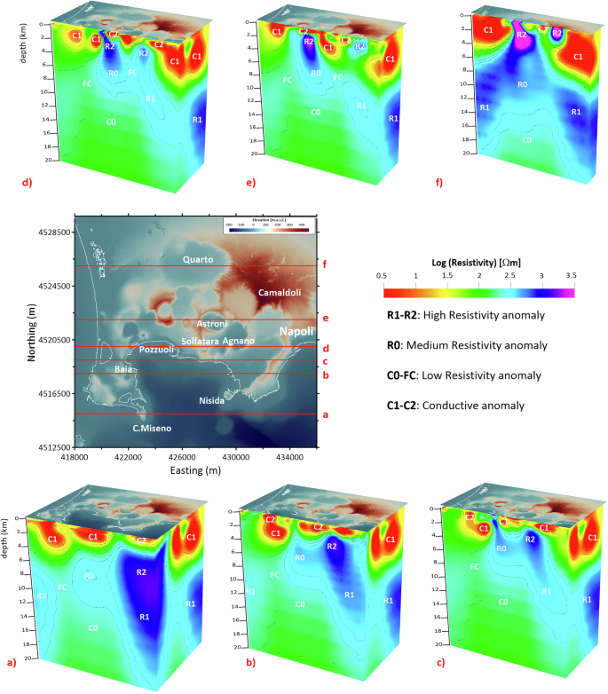
E-W sections (a–f) extracted from the model based on the magnetotelluric measurements; traces of the sections are superimposed on a digital elevation model of the Campi Flegrei area. All visualizations of the 3D resistivity models presented in this manuscript were produced using the ParaView software package.
The C0 zone exhibits variable width and thickness, with an estimated minimum iso-volume of ~915 km3. The top of this anomaly underlies the central sector of the caldera (Fig. 2a–d) beneath the relatively central Pozzuoli-Solfatara area and the feature gradually deepens. The R0 anomaly, located above C0, has an estimated minimum iso-volume of ~14 km³ and is laterally confined by the FC and R2 anomalies. The R2 anomaly is also present within the shallowest few kilometers of the crust, alongside the C1 and C2 anomalies. Towards the northern part of the caldera, the R0 zone transitions into the highly resistive R2. Moreover, the FC anomaly, with an estimated minimum iso-volume of ~80 km3, marks a lateral transition zone in the southwestern caldera sector between R1 on the west and R0 in the middle, and placed beneath the C1 anomaly. A similar but narrower transition (FC) is visible in the central portion of the model at shallower depths east of R0 (Fig. 2d, e).
Snapshot of a trans-crustal magmatic system
This new detailed 3D resistivity model of the Campi Flegrei caldera provides novel insights into the broad subsurface, particularly the size and geometry of the magmatic plumbing system and the volcano-tectonic features. The C0 anomaly beneath the caldera, extending between 8–20 km depth (Fig. 3), is consistent with a main melt accumulation zone exhibiting resistivity values and a geometry consistent with the feeding systems of other volcanic areas worldwide43,44,45,46. The top surface of the anomaly, at 8 km, may occur at a rheological discontinuity within the Campi Flegrei caldera, which could act as a permeability barrier allowing gases to escape to the surface and, thus, preventing magma ascent and promoting magma accumulation, as hypothesized for other plumbing systems47. The C0 anomaly occurs at a depth previously suggested for pre-eruptive Campi Flegrei magma storage based on petrological analysis of post-Neapolitan Yellow Tuff eruptions, as well as reconstructed deformation associated with the last eruption in 1538 CE (Monte Nuovo), and therefore likely represents the magmatic system that fed the recent volcanism32,48,49. The feature also correlates with previous geophysical estimates of Campi Flegrei magma storage based on seismic tomography33,34 (Supplementary Fig. S02) as well as interpretations of the recent fumarolic gas geochemistry50,51,52. Ground deformation from InSAR and GPS are consistent with inflation of source at around 8 km depth53,54.
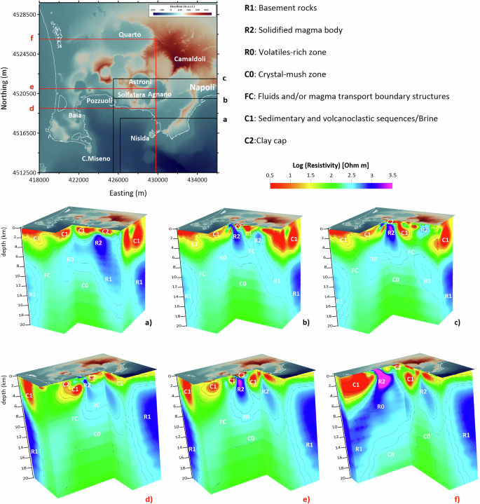
3D view of E-W and N-S sections (a–f) through the MT-based model image of the subsurface architecture beneath the Campi Flegrei caldera. The traces of the sections are superimposed on a digital elevation model of the Campi Flegrei area. The zones defined by different resistivities are interpreted based on depth and geometry and other geological petrological and geophysical observations. A low resistive zone (C0) is beneath in the central caldera, extending below 8 km, that is bounded to the E and W by high resistivity bodies (R1). C0 is interpreted to be a zone of crystal mush with some melt, and R1 is considered to be the basement rock. The middle to upper crust is comprised of various smaller zones of contrasting resistivity. The low resistivity zones that extend up to the shallow crust (FC) are interpreted as the zones that transport the fluids and melt/magma from the deeper part of the system. Some of these melts stall, degassing and crystallizing in the upper crust (R0), and alter the sedimentary and volcaniclastic sequences within the caldera (C1 and C2). R2 represents a solidified magmatic body related to the volcanism of the CF. All visualizations of the 3D resistivity model presented in this manuscript were produced using the ParaView software package.
Combining the electrical property of the C0 anomaly with estimates of the physicochemical characteristics of Campi Flegrei magmas in the mid-lower crust, it is possible to estimate the melt fraction within the magma storage zone (see Methods)55. This analysis indicates that the C0 has a melt fraction of ~10% and contains ~90 km3 melt within its total volume. At these low melt fractions the C0 anomaly records a transcrustal, crystal-rich mush zone beneath the Campi Flegrei caldera, consistent with recent interpretations of other major caldera-forming volcanoes56.
C0 is laterally confined by R1 that is observed on both the E and W sides and extending below the modelled region, likely corresponding to the basement rocks (Fig. 3), composed of crystalline bodies, flysh and/or limestone of the Apennines that outcrops along the edge of the Campanian Plain and below the nearby Somma Vesuvius volcano. Above C0, the R0 anomaly could be interpreted as an area of basement rock altered by the significant circulation of magmatic fluids above the main zone of magma storage (as for other active volcanic systems)46,57, or a zone of near- or sub-solidus igneous rocks formed from the residue of past eruptions and/or solidified minor sills ascended from depth before stalling and solidifying (Fig. 3a–c). Lithics included in eruption deposits testify to there being altered rocks, sedimentary flysch, and intrusives in the shallow crust58. The upper part of R0 corresponds to a region with low VP/Vs values59, where previous studies have identified ephemeral sills, either prior to recent eruptions32,52 or during recent unrest crises37; most of the ongoing seismic swarms and highest magnitude earthquakes are located at the boundary of R0, along the FC structures and at the bottom of R2 (Fig. 4).
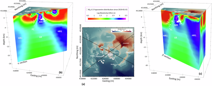
The (a) shows the map of the CF area, with elevation represented by a color scale and epicentres of earthquakes (Md > 2.5, since January 2019; white dots). The black lines indicate the α and β profiles used to extract the 3D resistivity sections. b, c display the resistivity cross-sections along α and β profiles, with hypocentress of earthquakes superimposed (white dots). All visualizations of the 3D resistivity models presented in this manuscript were produced using the ParaView software package.
The physicochemical parameters of the magmas that reside at these depths and the electrical properties of R0 volume indicate a maximum ~0.4 km3 of melt, which corresponds to a melt fraction of ~3%55. Our results don’t preclude the presence at shallower depth of small melt volumes below the resolution of the modelled image, as ephemeral sills (Methods).
The R0 anomaly is bordered by the two thin zones with lower resistivities (FC) (Fig. 3a–e). These anomalies connect C0 with the C1, especially in the central-western sector of the caldera (Fig. 3a–e). They correlate with regional-trending features that are exposed at the surface, which have functioned as volcano-tectonic collapse structures during the large caldera-forming eruptions of Campi Flegrei29. We therefore suggest that these FC anomalies represent deep fluids and/or melt zones, that are exploiting tectonic features (Fig. 3a, e). As for C0, we estimated the melt fraction possibly included in the FC structure as ~8% of its volume corresponding to ~6 km3 of melt. The movement of magmatic fluids and/or melt, from the top of the C0 anomaly along these features could be responsible for the lower resistivity values of R1 in the western sector of the model, due to the related thermal effects (Fig. 3a–e). The deepest hypocenters recorded during the ongoing unrest31 are located on top of FC anomaly (Fig. 4), which suggests that these features could represent structural boundaries along which magmatic fluids/melt could rise, as seen at other volcanoes47.
Several conductive anomalies (labeled C1 and C2 in Figs. 2, 3) with different widths and thicknesses have been imaged across the shallowest parts of the model above R2. Within the caldera, some of these anomalies (Fig. 3a–e) are likely associated with young sedimentary caldera-infill and/or volcanic rocks which have undergone alteration as a result of magmatic fluids rising through the FC structures (C1; e.g. brines and/or hypersaline fluids; Fig. 3a, b, e). The geometry and location of C2 (mainly in the central sector; Fig. 3b–e) can be associated to a present-day alteration zone related to an active hydrothermal/fumarolic system; it has the characteristic clay-cap structure, which has also been identified in previous short-period MT surveys across the area60,61. Notably, the vertical resistivity contrasts detected in the shallowest part of the model correspond with volcano-tectonic features associated with the recent intra-caldera volcanic activity (Fig. 3d, e and (Supplementary Fig. S03).
The geometry of the Campi Flegrei geothermal system as revealed by the 3D MT tomography is consistent with the temperature distribution recorded inside the caldera. Explorative boreholes drilled by Agip in the 1970s observed the highest temperature gradients in the Mofete well field (Fig. 4), in the vicinity of a prevalent conductive zone (C1). In contrast, a shallower geotherm was identified in San Vito wells which correlate with more resistive features62 (R2).
At shallow crustal levels, R2 is likely associated with a partially or entirely cooled magmatic body. The uppermost part of R2 in the central sector of the caldera is close to the Rione Terra district of Pozzuoli town (Fig. 3c–d), and could be related to an arrested magma intrusion that may have caused the 1982-84 unrest crises. Northwards, R2 anomalies occupy the shallowest 3 km of the model’s central sector, where a significant positive magnetic anomaly has also also been detected39, suggesting that magmas likely intruded through a North-South trending extensional structure (Fig. 3e–f).
There is a sharp change in the geometry and dimension of anomalies in the northernmost sector of the imaged area, which lies outside the Neapolitan Yellow Tuff collapse structure and vent locations for post-15 ka eruptions (Fig. 3f). Here, there is a generally more resistive environment, and the C0 anomaly is deeper and smaller. This suggests that the magmatic fluids are limited to within the caldera area, consistent with the absence of active hydrothermal and/or fumarolic activity at greater distances.
Implications for hazard management
Our new 3-D resistivity model extends to a depth of 20 km beneath the Campi Flegrei caldera and reveals electrical resistivity anomalies that can be attributed to distinct physical structures within the sub-volcanic system. The configuration and properties of these anomalies indicate the presence of a transcrustal magmatic system, in which magma accumulation extends over a large vertical distance within the crust (Fig. 5).
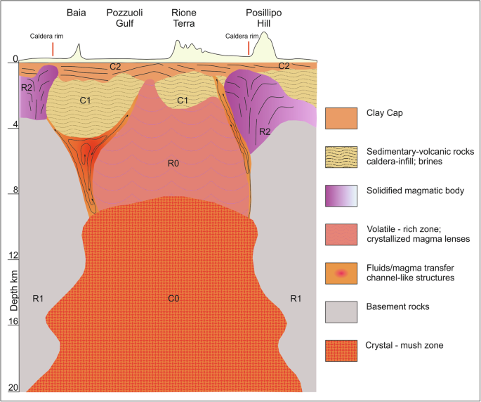
Interpretative scheme of the magma plumbing system and subsurface structures beneath Campi Flegrei after the 3D MT model.
The architecture of the transcrustal system beneath the Campi Flegrei appears to be characterized by a low resistivity anomaly (C0) in the middle-lower crust that extends from ∼8 to >20 km depth, representing the main melt accumulation zone. A medium resistive (R0) zone and channel-like structures (FC) are also interpreted as part of this transcrustal magmatic system, where melt/magma intruded in the past and has partially or completely cooled/crystallised. These old intrusions are thought to have generated seismic unrest and fueled at least some of the bradyseism that has been historically experienced in the caldera region30,37; the epicentres of many Campi Flegrei earthquakes are located along the upper edge of the FC and R0 anomalies (Fig. 4 and Supplementary Fig. S02).
Our results contribute to resolving open issues about the magmatic system beneath the active Campi Flegrei caldera and place new constraints on the location, volume, and geometry of both the deep and shallow magmatic/hydrothermal plumbing systems. Our findings also identify subsurface structures that likely facilitated magma and hydrothermal fluid migration during past episodes of unrest, which we propose might play a role during future unrest. The emerging subsurface image of the Campi Flegrei caldera has a three-tier crustal structure with: (i) a spatially confined deep zone of magma storage containing melt within a crystal-mush (>8 km depth); (ii) an intermediate-depth (3–8 km) zone containing crystallized magma lenses and fluid/magma-rich channel-like structures along the major volcano-tectonic features; (iii) a shallow (<3 km depth) zone of containing altered caldera-fill that has interacted with circulating deep-sourced magmatic fluids (clay-caps), accumulated high-salinity fluid (brines), and crystallised or partially crystallised magmatic intrusions. Such a model (Fig. 5) defines a plumbing system where deep crystal mushes are connected to a shallow hydrothermal system mainly through channel-like structures which act as transfer zone (for magmas or magmatic fluids). Magma at depth between 3–8 km resides and/or propagates as small melt-rich lenses with a spatial scale below the resolution of our geophysical methods (see “Methods”). Our results strongly contribute to the interpretation of monitoring data that heavily relies on understanding the architecture of the plumbing system. The imaged transcrustal system (in terms of volumes and geometries) could furnish new elements for volcano monitoring strategies (e.g. surveillance network configuration, new geochemical and magnetic site measurements, etc.), also assessing the changing state (e.g., ground deformation, degassing, seismicity) and processes within the magmatic system which could lead to eruptive crises (e.g., the transfer of magma toward the surface).
Methods
Data acquisition and processing
The Campi Flegrei caldera was explored by an electromagnetic field campaign performed during 2022–2023. MT is a frequency-based standardized geophysical technique that reconstructs the electrical resistivity distribution by analyzing the synchronous fluctuations of the electric and magnetic fields that are naturally induced in the subsoil by external sources. A vast amount of literature exists that describes the basic principles of the MT and its practical aspects (e.g63,64).
Data were collected during fieldwork at on-shore 42 and six off-shore measurement points (Fig. 1b). The on-shore MT surveys were realized using three ADU08 five-channel stations produced by Metronix®, equipped with BF4 induction coils. The two perpendicular horizontal magnetic field components, Hx and Hy, and the vertical magnetic field component, Hz, were recorded at each site. Additionally, the two perpendicular horizontal electric field components, Ex and Ey, were measured using non-polarizing Pb–PbCl lead–lead chloride electrodes laid out in a cross with a dipole length of at least 100 m. The time series were recorded overnight for at least 12 h at a sampling frequency of 8 Hz, and at least another 2 h at a sampling frequency of 2048 Hz. The three stations were simultaneously deployed in the field, permitting cross-referencing of the surveys65. The geomagnetic surveys were realized off-shore using a Lemi-301 flux-gate magnetometer produced by the Lviv Centre Institute for Space Research of Ukraine and the National Space Agency of Ukraine (LCISR of NASU and NSAU). The instrument has a flat response curve, at least at periods greater than 1 s. The magnetometer was lowered to the seabed of the Pozzuoli Gulf between 40 and 50 m depth. At each marine site, magnetic signals were acquired for 15 days. The GPS-synchronized Lemi-301 is equipped with a built-in tiltmeter, which was employed to rotate the acquired signals along the magnetical main axes.
The acquired raw time series were processed via the RMEV multivariate technique65, taking advantage of the simultaneous data acquisition66. One of the three land stations was always located in a selected remote location, which resulted in a quiet site scarcely affected by coherent electromagnetic noise. In such a way, the (complex) transfer function Z, known as the ‘impedance tensor ‘, has been estimated by applying the relation: ([{E}_{x}quad {E}_{y}quad ]=[{Z}_{{xx}}quad {Z}_{{xy}}quad {Z}_{{yx}}quad {Z}_{{yy}}quad ][{H}_{x}quad {H}_{y}quad ]). Also, the induction vector T, known as the tipper function, has been estimated through the relation: ({H}_{z}=[{T}_{x}quad {T}_{x}quad ][{H}_{x}quad {H}_{y}quad ]). Once estimated Z, the curves of apparent resistivity (ρa) and phase (φ) have been derived, which can be defined as:
where μ and f are the magnetic permeability and the frequency, respectively. Examples of sounding curves (apparent resistivity, phase and tipper) are reported in Supplementary Fig. S04.
A critical aspect of MT data processing involves identifying and managing anthropogenic noise that may distort the true subsurface resistivity signal. In our analysis, we observed patterns consistent with noise interference, which could affect the reliability of the inversion results. The impact of noise on MT data has been extensively documented, with recent studies by Di Giuseppe et al. 66 providing valuable insights into the spectral characteristics and eigenvalue distributions that typify noise-affected data in the investigated area. Using the spectral density matrix approach, we evaluated the frequency dependence of noise in our dataset, as illustrated in Fig. 6. The spectral analysis allowed us to detect frequency bands where noise dominates, which tend to correspond to frequency ranges that are commonly associated with anthropogenic sources64. By focusing on the higher signal-to-noise ratio, we aimed to isolate the signal-dominant regions and reduce the potential influence of noise in the inversion. For such purposes, we used eigenvalue analysis to assess noise contributions across different sites. Figure 6 (from the eigenvalue analysis of66) illustrates the characteristic structure in the eigenvalue distribution, which reflects the relative importance of the signal versus noise. In our dataset, sites exhibiting higher eigenvalue numbers suggested strong noise presence, likely due to external, non-geological sources. As a consequence, the pattern of Fig. 6 served as a diagnostic tool to identify and selectively exclude data from sites where noise was predominant, ensuring that the retained data more accurately represented the subsurface resistivity structure. Furthermore, we adopted the stability of the spectral density matrix eigenvector direction as a criterion to evaluate the quality of the data.
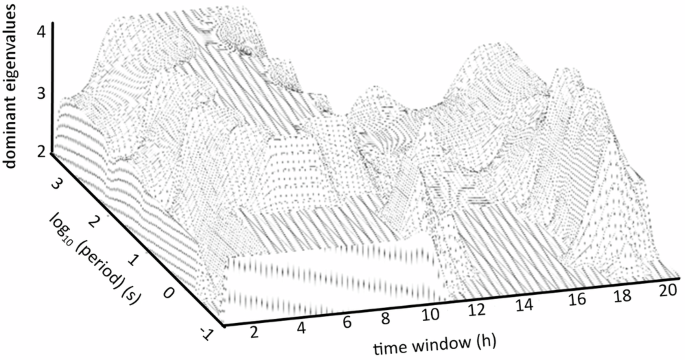
Dominant eigenvalues number versus time (h) and period common logarithm (s) representative of the MT data quality. The collected time series (having a duration of ~23 h) have been separated into shorter contiguous time windows. Subsequently, the RMEV estimator has been applied to every time window, estimating the number of dominant eigenvectors vs. period.
Data analysis
The dimensional dataset analysis was performed considering the phase tensor PT67, which analogously to the impedance tensor Z defined before, can be defined as:
({PT}=left[{Phi }_{{XX}} {Phi }_{{XY}} {Phi }_{{YX}} {Phi }_{{YY}} right]), where each element Φi,j is given by (left(frac{{Im}left({Z}_{{ij}}right)}{{{mathrm{Re}}}left({Z}_{{ij}}right)}right)).
PT is insusceptible to galvanic distortions and can be represented graphically as an ellipse with the principal axes (Φmax and Φmin) showing the major-minor axes of the tensor. The polarization ellipses behaviour, estimated through the MTpy code68,69, has been reported for selected periods in Fig. 7. Such ellipses can be employed to estimate which parts of the impedance tensor could be considered 1D, 2D, or 3D once the ellipticity (λ) and, in the case of nonsymmetry, the skew-angle (β) has been defined as a function of Φmax and Φmin70. For every single period, the dimensionality of the MT dataset can be evaluated according to the criterion: 1D): λ ≈ 0, β ≈ 0; 2D): λ ≠ 0, β ≈ 0, (α-β) constant; 3D): λ ≠ 0, β ≈ 0 or β ≠ 0, but (α-β) no constant71. A threshold value has been considered for the skew angle β (5 degrees) and the ellipse’s eccentricity λ (0.1). Such a PT analysis confirms the 3D character of the subsurface below Campi Flegrei caldera. The characteristics of the PT polarization ellipses and the induction arrows are discussed below, taking into account the characteristics of the 3D resistivity model obtained through the data inversion.
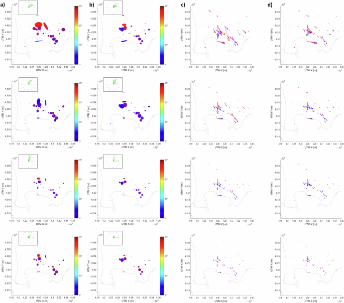
Maps showing the Phase Tensor Polarization ellipses (columns a and b) and induction arrows (columns c and d) across various periods, highlighting both observed and predicted values. Columns A and C present the values derived from the field MT data, while columns B and D display those obtained from the synthetic response of the 3D resistivity model inverted using ModEM. Each row corresponds to a distinct period (1 s, 10 s, 100 s, and 1000 s), providing insights into the evolution of polarization and induction patterns with depth. The colors of the ellipses indicate the phase angle β (degrees), with the accompanying color scale shown on the right. Rose diagrams of the β angle are also reported. Induction arrows reflect the direction and strength of subsurface conductivity, with blue arrows representing real components and red arrows representing imaginary components, plotted using the Parkinson convention.
Afterward, the influence of the ground-level topography and seafloor bathymetry on the dataset was evaluated following the same procedure already developed by61 for the case of a similar application realized in the central sector of the Campi Flegrei caldera. The results of such an analysis were considered during the inversion phase when the choice of error floors imposed on the data was made.
Data inversion
As previously described, the processed MT signals yielded apparent resistivity, phase, and tipper curves, estimated over the period band of 0.1–1000 s. This dataset was resampled into 17 logarithmically-spaced periods to unburden the time-consuming 3D computation. The resampling was calculated using a routine in the MTpy toolbox68,69; specifically, the routine mt_obj.interpolate, which interpolates the impedance tensor onto different frequencies. The parallel version of the 3D code Modular system for Electromagnetic inversion (ModEM)72,73,74, has been employed for data inversion, which was run with full impedance tensor and tipper elements (Zxx, Zxy, Zyx, and Zyy; Txx and Tyy). Inversion with different settings was executed using 90 cores (nine nodes) of the high-performance computing INGV (HPC) cluster.
The inversion settings, the 3D mesh, and the results were prepared and analyzed using the 3D-GRID Academic software74. The domain was 130 km in the horizontal directions away from the model center and around 200 km deep, consistent with the boundary conditions and the electromagnetic skin depth. The model mesh adopted during the inversion of our dataset includes bathymetry and topography and contains: 50 cells in the north-south direction, 50 in the east-west direction, and 70 in the vertical direction (plus ten air layers). Layers above sea level have a thickness of 50 m, and the first layer below sea level has a thickness of 100 m and the thickness increases by a factor of 1.2 for each subsequent layer down to a depth of 3 km. The first layer below a depth of 3 km has a thickness of ~500 m, increasing by a factor of 1.3 for each subsequent layer. It is worth noting that our choice of maximum vertical mesh depth was informed by the Niblett-Bostick depth estimation, which is detailed below.
The core mesh contains 300 m by 300 m horizontal cells, allowing room for multiple model cells between stations. The high-resolution bathymetry of the Campi Flegrei coastline was included as a priori information and kept fixed during the inversion. A resistivity value of 0.3 Ωm was used for the seawater. Model regularization employed a smoothing parameter of 0.4 for horizontal and 0.3 for vertical directions.
Due to the non-unique solution of the inverse problem, various tests were conducted to work out the starting model and the smoothing factors. Following the most recent literature findings, these settings were chosen and adapted to our specific dataset. As a preliminary step in the inversion process, we conducted several ModEM runs using starting models with homogeneous resistivity values. These initial resistivities were set to 1, 10, 100, 1000, 10,000, or 100,000 Ωm. As said before, a 0.3 Ωm resistivity was assigned to the seawater. For these inversions, we applied broad error bars. We observed two types of behavior: the central resistivity values (e.g., 100 Ωm) tended to converge toward similar models, while the higher and lower resistivity values failed to converge. Ultimately, we selected 100 Ωm as the starting resistivity for our model, as it provided the best convergence behavior.
Each datum used in the inversion was assigned an error, estimated as a fixed percentage of the data value. The ModEM inversion aims to minimize the misfit of each datum; if error estimates are too large, the inversion may inadequately fit the measured data, while overly small error estimates may cause noise to be fit, resulting in a rough model. Standard impedance errors derived from time-series processing can be minimal compared to the impedance values, making it necessary to apply an error floor to achieve a satisfactory inversion result. In our case, we diversify the uncertainty applied to diagonal and nondiagonal modes of the Z tensor, setting an error floor as a portion of the absolute value of the impedance components. An error floor of 5% for the off-diagonal components and 10% for the on-diagonal components has been chosen. The error floor of the tipper components was assigned as 10% of the absolute value.
For this first inversion model, 60 interactions were required to fit the full impedance tensor and the tipper. As a metric for the fit of the modeled to the observed data, the commonly used normalized root mean square (nRMS) has been adopted, which is defined as:
where dobs,j and dcalc,j are observed and calculated data, respectively, and σj represents the errors for all Nd data points. A value of this metric close to 1 is commonly interpreted as a data fit within the range of observational error, that is, in the case of this study, the error floors. A final nRMS, which achieved a value of ~1.3.
After this first inversion, we noted that by analyzing the MT data from our survey, it is possible to identify some primary patterns in the apparent resistivity and phase curves (see Supplementary Fig. S05 and Table S01). The first pattern is characterized by a monotonic increase (MI) in resistivity with depth, suggesting undisturbed geological signals. A second pattern shows a more oscillatory behavior, with resistivity values fluctuating within a specific range (Intermediate-Low-High; ILH); such oscillations may indicate minor geological complexities or possible low-level anthropogenic noise.
We employed an iterative approach to ensure our inversion model’s reliability. The first inversion, described before, included data from all sites (Fig. 1b), allowing us to capture a preliminary model of the main resistivity structures. We then conducted a second inversion, excluding data from sites displaying the pattern more prone to irregular features potentially associated with noise (yellow points in Fig. 1b). This selective exclusion allowed us to refine our model by reducing the influence of suspect data while preserving meaningful geological information. The comparison between the first model (including all sites) and the refined model (excluding sites with irregular features) showed substantial similarity in the primary resistivity structures, demonstrating the robustness of our inversion results. For the final interpretation, we chose the model derived from the inversion excluding these specific sites, achieving a balance between reducing potential noise effects and accurately representing the subsurface structures. For this final inversion model, 75 interactions were required to fit the full impedance tensor and the tipper. Figure 8 shows a map of the final nRMS, which achieved a value of ~2.15. The overall quality of the data fitting can also be deduced from the curves presented in Supplementary Fig. S06. All significant inversion parameters are reported in Supplementary Table S02.
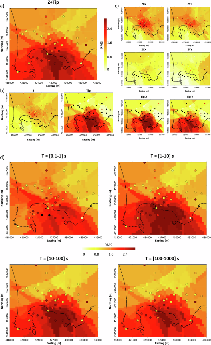
Maps of normalized root mean square (nRMS) values for the whole dataset (a), the individual tensor elements, and the tipper (b) provide insight into the contribution of each component (c) to the overall fit. In contrast, period band maps for selected bands (d) highlight the spatial distribution of model misfits at varying penetration depths. The color scale used to represent nRMS values is included.
PT analysis
The polarization ellipses and induction arrows at various periods, shown in Fig. 7, provide an overview of the resistivity structure in the Campi Flegrei area, as derived from both field measurements and the 3-D resistivity model. The field-derived induction arrows generally point towards regions of lower resistivity, indicating the presence of conductive zones, which align with known geological features in the area. The polarization ellipses, with their size, orientation, and color-coded phase angles, reflect the variation in resistivity and phase response across different sites and periods.
In comparing the measured and predicted values, we observe a generally good alignment between the two, suggesting that the 3D resistivity model accurately captures the main conductive structures indicated by the field data. The induction arrows emphasize the conductive anomalies within the Campi Flegrei caldera. The arrows aligning well with known conductive zones and geological structures. However, some discrepancies are observed between the measured and modeled data, particularly at intermediate periods (e.g., 10 s and 100 s). These differences are more pronounced in the induction arrows, where the observed orientation and magnitude deviate from the model predictions in certain areas. Such variations could be likely attributed to small-scale heterogeneities. In regions where the ellipses are highly elongated or the induction arrows are strongly clustered, the resistivity model captures the dominant conductive structures reasonably well.
Resolution tests
The consistency of the main features of the preferred inversion model was questioned by performing a series of tests in order to analyze every significant structure separately.
First, we adopted the MTpy code to evaluate the penetration depths of the electromagnetic waves at a 10 s period, using the Niblett-Bostick transform (68 and references therein), which map is reported in Fig. 9.
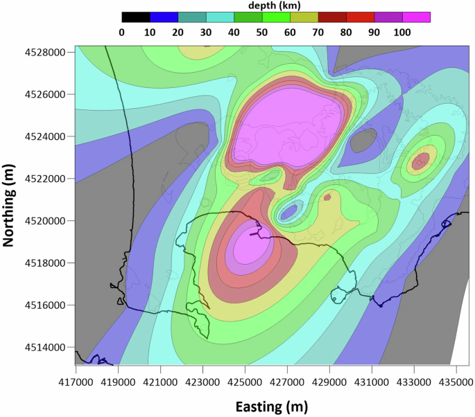
Map of the penetration depth of the electromagnetic waves of 10 s period, obtained using the Niblett-Bostick transform.
In the second step, we performed sensitivity tests on certain parts of the model. Due to the complexity of 3D, the model perturbation method has been used to assess the sensitivity and robustness of our preferred model. We performed a series of targeted sensitivity tests, following these steps:
-
(i)
Selection of Key Structures: we identified the primary conductive and resistive structures in our preferred model that are most relevant for the geological interpretation of Campi Flegrei. These included regions of interest such as potential melt zones, hydrothermal systems, and deeper resistive layers that may represent crystalline or partially solidified rock.
-
(ii)
Modification of Resistivity Values: we systematically modified the resistivity values for each selected structure to create alternative model versions. Specifically, we either increased or decreased the resistivity within the targeted zones by several magnitude orders to simulate possible variations in the subsurface resistivity. This range of modifications allows us to assess how much the model’s resistivity values influence the overall inversion outcome.
-
(iii)
Forward Modeling: using the modified resistivity values, we performed forward modeling to generate synthetic apparent resistivity and phase curves for each alternative model. By maintaining consistent model parameters, we ensured that any observed variations in the responses were due to changes in resistivity within the targeted structures.
-
(iv)
Comparison of Modeled and Observed Curves: we then compared the synthetic curves from the forward models with the observed data, focusing on discrepancies in apparent resistivity and phase. By analyzing how the modified resistivity values affected the fit of the curves, we could identify which structures were sensitive to resistivity changes and which were less constrained. High-sensitivity regions showed significant deviations in the modeled curves when resistivity was adjusted, indicating that the original values were critical to matching observed data. We adopted the nRMS misfit metric to evaluate how changes in resistivity affected the model’s fit to the observed data. Regions where resistivity modifications led to substantial deviations in the forward response were considered well-constrained and robust. Conversely, areas where changes had minimal effect were marked as zones with greater uncertainty, and interpretation should be cautious.
The following features have been questioned: i) a low resistivity anomaly, C0, characterized by a few hundred Ωm values, extending to the maximum investigation depth of the model; ii) the circular anomaly of medium resistivity, R0, located between 8 km and 3 km depth; iii) the channel-like zone, FC, with resistivity values similar to C0; iv) the off-shore part of the model. The results of the resolution test are summarized in Supplementary Fig. S07.
Figure 9 and S07 are essential for evaluating the sensitivity and reliability of our preferred model. The map of penetration depths of electromagnetic waves at a 10 s period provides an estimation of the depths reached by electromagnetic waves at this period, offering insight into the effective sampling depth of our MT data. This information is crucial for understanding the model’s depth sensitivity, as it highlights the regions where the resistivity structure can be reliably resolved. By establishing the maximum penetration depth, we can more confidently interpret resistivity features at various depths, knowing that our data provides adequate sensitivity within these zones. The results of sensitivity tests allow us to assess the robustness of the resistivity features within the Campi Flegrei model, indicating zones where interpretation is reliable and where it should be approached with caution.
Implications for melt fraction
Hypotheses about the physical state of the magma crystal mush identified by the 3D resistivity model in correspondence with C0, FC (Fig. 3; both ∼125 Ωm) and R0 (Fig. 3; ∼650 Ωm) anomalies were deducted by adopting the approach proposed by55.
While specific studies of the electrical properties of trachytic Campi Flegrei magmas are lacking, we can use the existing literature concerning chemical analyses of melt inclusions associated with different caldera eruptions to gain insight into this matter. The bulk resistivity of magmatic rocks ρbulk, generally depends on several factors, particularly the composition, crystal fraction, and geometry of the melt portion75. The intrinsic resistivity of the melt depends primarily on its water content and sodium ion concentration76,77. The SIGMELT software76 allows the resistivity of a silicate melt to be quantified based on its composition and the state of the partially molten material in terms of temperature and pressure. These conditions are reported in Table 1 for our case, including the water, sodium, and silica content and the corresponding pressure and temperature22,32,78 for the three identified anomalies. A plausible estimate of the mean electrical conductivity of the melt ρmelt, can be derived from these data.
To substantiate the observed electrical resistivities corresponding to the C0, FC, and R0 anomalies, we can estimate the resistivity of the rock matrix, which is critical for formulating hypotheses about the observed bulk resistivity (Fig. 10). Assuming the rock in adjacent formations has a common resistivity of ~1000 Ωm, various models can reconstruct the resistivity of two mixed phases (melt and crystallized rock matrix).
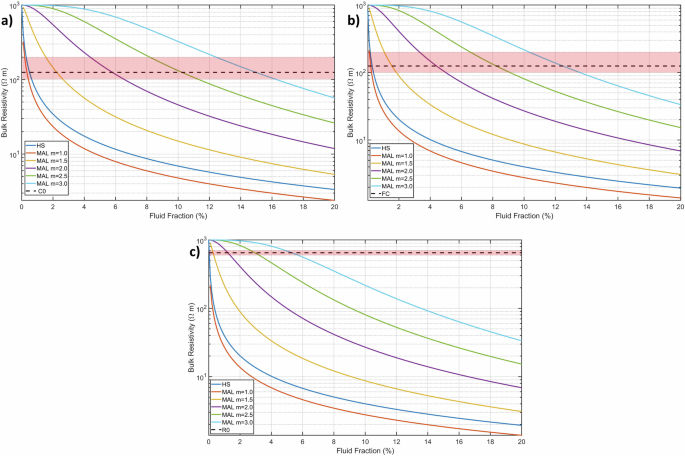
Bulk resistivity as a function of fluid fraction. The colored lines represent the bulk resistivity, calculated using Hashin-Shtrikman (HS) and Modified Archie’s law (MAL), with different cementation factors m for the conditions reported in Table 1. The black dashed lines indicate the bulk resistivity of 125 Ωm for the C0 (a) and FC (b) anomalies and 650 Ωm for the R0 anomaly (c); the pink shaded area represents the bulk resistivity range for each feature.
In this study, we employed the Modified Archie’s Law (MAL) to estimate melt fractions in partially molten regions at Campi Flegrei79. Although MAL was originally developed for clay-rich environments, it has been widely adapted in geological contexts where the connectivity of a conductive phase, such as an interconnected melt network, significantly influences bulk resistivity80. Given the role of partial melt connectivity in the resistivity structure at Campi Flegrei, MAL is suitable for estimating melt fractions within our model, as it accounts for the influence of conductive phase connectivity on overall resistivity. Additionally, we considered using the Hashin-Strikman (HS) bounds81, which provide theoretical upper and lower limits for effective resistivity in heterogeneous media. However, given the observed conductivity patterns and partial melt characteristics in this region, we found MAL to be an effective approach for capturing the main features of melt fraction distribution. Figure 11 reconstructs the behavior of the bulk resistivity as a function of the fluid fraction percentage for the Campi Flegrei rocks, obtained through the application of the HS and the MAL, which considers various cementation factors m to denote the degree of phases interconnection82,83. We suggest that the C0, FC, and R0 resistivity anomalies are consistent with a melt fraction of ~10%, 8%, and 3%, respectively (Fig. 10). The chosen melt fraction values for C0, FC, and R0 anomalies were based on experimentally and empirically observed ranges in partially molten systems. These values represent plausible estimates for melt fraction under different connectivity scenarios and reflect expected variability in the distribution and connectivity of melt. By applying these values, we aim to provide a robust approximation of melt fraction, which can be important for understanding magma mobility and the potential for eruptibility in this complex volcanic system.
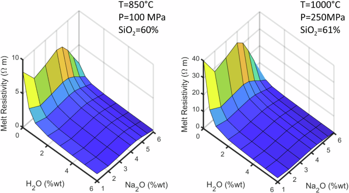
Plot of the melt resistivity (Ωm) vs. H2O and Na2O content (%wt) determined using the SIGMELT tool (see Table 1 for values). The pressure and temperature conditions and the silica content are extrapolated from Table 1 for the FC and R0 structures (on the left) and the C0 structure (on the right).
Analysis of Melt Resistivity as a Function of H2O and Na2O Content
To assess the influence of compositional variability on melt resistivity, we examined how melt resistivity varies as a function of water (H2O) and sodium (Na2O) content within ranges relevant to the Campi Flegrei magmatic system22,32,78. This was estimated using the SIGMELTS tool to calculate the resistivity of melt at the temperature chosen for our model, specifically 850 °C and 1000 °C (Table 1). These temperatures were selected to be consistent with the estimated conditions of the R0, FC, and C0 structures in our melt fraction analysis. This analysis is presented in Fig. 11. In the calculated range, we observe a gradual decrease in melt resistivity as both H2O and Na2O content increase. This trend is consistent with the well-documented role of water in enhancing melt conductivity, as it facilitates ionic mobility84,85. Sodium also contributes to reducing resistivity, though to a lesser extent than water, likely due to differences in ion mobility and the overall effect on melt structure. Importantly, no discontinuities were observed in the resistivity values across the studied compositional range. The absence of sudden changes or jumps in resistivity indicates that, within these intervals, the melt’s conductive properties change in a continuous manner without undergoing abrupt structural transitions or phase changes. This smooth variation suggests that, for the purposes of our model, melt resistivity can be assumed to vary predictably with compositional changes in H2O and Na2O content. This behavior supports the reliability of our model’s melt resistivity assumptions and simplifies the interpretation of the magnetotelluric data, as it indicates a stable conductive response across the range of compositions examined.
Conductance sensitivity and melt fraction estimation
The MT method is primarily sensitive to the conductance of subsurface layers, which is the product of conductivity and thickness64,86,87. As a result, MT data inversions typically resolve conductance rather than absolute conductivity, creating a trade-off between layer thickness and conductivity. In our 3-D inversion, we employed the ModEM algorithm, which uses Tikhonov regularization to stabilize the inversion process by applying a smoothness constraint. This regularization can result in conductive layers appearing thicker and less conductive than they may actually be in the Earth. This imposed smoothness introduces a significant limitation when estimating melt fraction in partially molten regions88, leading to a risk of underestimating the true conductivity of a melt-bearing layer and potentially underestimating the melt fraction. In volcanic hazard assessments, this could suggest a lower melt fraction and, consequently, a lower potential for magma to be in an eruptible state.
In our case, we can conclude that the melt fraction in the partially molten region we model may be underestimating melt fraction due to smoothing, as well as to the minimum assessment of the C0 volume due to maximum depth penetration of the model.


Responses