Neonicotinoid insecticides can pose a severe threat to grassland plant bug communities

Introduction
We are facing an unprecedented decline in biodiversity, which has been particularly evident for insects in recent years, with many studies showing global declines in insect biomass, abundance, and richness1,2,3,4,5. The intensive use of agrochemicals is considered to be a major driver of insect decline5,6,7. Non-target insects can be exposed to insecticides in both agricultural and non-agricultural areas. For terrestrial insects, direct contact and oral uptake are likely the main routes of exposure. Direct contact can occur through overspray or contact with plant or soil surfaces containing residues. Oral uptake can occur through the consumption of contaminated food, e.g. plants or other invertebrates8. In terrestrial non-target habitats (e.g. field margins, neighbouring meadows, hedges), such exposure is mainly caused by overspray and spray drift9. Although atmospheric transport of pesticides can lead to deposition even in remote areas such as alpine environments10,11, areas close to the field such as field margins, are particularly affected, since the first metre of a field margin is exposed to both overspray and spray drift. Estimates of pesticide deposition here range from 30% to 58% of the field rate9,12. At the same time, semi-natural habitats such as field margins make up a significant proportion of insect habitats in modern agroecosystems13. It is, therefore, all the more alarming that there is increasing evidence that modern agroecosystems, as well as non-agricultural landscapes and even insects in nature preserves, are contaminated with pesticides14,15,16.
While the exposure of non-target insects to pesticides may seem obvious, its impact is poorly understood. Although modern insecticides should ideally be less toxic to beneficial insects such as the Western honeybee Apis mellifera than to the target pest (e.g. based on the German bee risk management levels B1–B4), sensitivity to insecticides can vary even between closely related species and is generally difficult to predict17,18. The current EU insecticide registration protocol requires sensitivity testing for a limited number of non-target insects. These are typically the honeybee, parasitic wasps, predatory mites, and individual representatives of beetle families such as the Coccinellidae, Carabidae or Staphylinidae19. Furthermore, the vast majority of available ecotoxicological studies involve either aquatic invertebrates or terrestrial beneficial insects such as pollinators or predators20,21,22. Herbivorous insects, which account for about 50% of all insect species globally, have been largely neglected23,24. Another shortcoming in the ecotoxicological literature is the underrepresentation of community-level studies, i.e. the evaluation of a range of species with different sensitivities within the same habitat. The study of community-level effects in realistic exposure scenarios is an important cornerstone for assessing the true ecological consequences of insecticide contamination. Consistent community structure effects of insecticide exposure have already been shown for aquatic systems21. However, comparable studies for terrestrial systems are largely lacking, and the few that do exist tend to focus on soil invertebrates25,26,27.
In this study, we address the existing research gap on insecticide exposure of non-target herbivorous insects, focusing on two main aspects: (1) realistic exposure scenarios, (2) community-level effects, i.e. differential sensitivity between closely related species and between sexes of the same species. We chose plant bugs (Heteroptera: Miridae) as a model group because they are one of the 20 most diverse insect families and a common component of non-target insect communities in agroecosystems28,29. Plant bugs are highly abundant in meadows, but can also be found in grassy field margins, as many species are associated with Poaceae28,30. The high diversity and abundance of this group suggest an important function for the ecosystem. However, this group of insects is understudied in terms of non-target effects of insecticides, with the existing literature focusing exclusively on agriculturally relevant beneficial species (i.e. predatory species)31,32,33 but not on plant bug species primarily occurring in off-field environments. In addition, plant bugs are not considered in the risk assessment procedure for plant protection products. We argue that plant bugs are an ecologically relevant group to study. They are most certainly an important food source for birds and a wide range of predatory invertebrates34. In addition, species within plant bug communities are often similar in many traits (e.g. morphology, habitat, diet, and phenology) and therefore offer the opportunity to study physiological differences in insecticide sensitivity at the species level due to the high diversity of this family28.
We conducted field, greenhouse, and laboratory experiments to mimic insecticide exposure in different scenarios. We used the neurotoxic neonicotinoid insecticide Mospilan®SG with the active ingredient acetamiprid (200 g/kg) in all experiments. Mospilan®SG is applied by spraying and is used in field crops such as rapeseed and potato, in orchards, in wine growing and in floriculture, in particular against chewing-sucking pests. The active substance acetamiprid is both a contact and a systemic insecticide, as it can also be absorbed by plants and distributed throughout their tissues. Among other neonicotinoids, acetamiprid is used worldwide, but in the European Union, it is the only neonicotinoid still registered for open-field use. The global acetamiprid market size is estimated at USD 118 million in 2022 and is expected to grow significantly35.
In the field experiment, we sprayed three concentrations of Mospilan®SG in semi-open field enclosures with wild plant bug populations to simulate in-field and off-field exposure scenarios (Fig. 1a). The enclosures were located in an extensively managed meadow in southern Germany. We selected treatments based on deposition estimates as follows: ‘100%‘ = typical field rate of 250 g/ha in 600 l of water (e.g. as used for potatoes, cabbage, or lettuce); ‘30%‘ = exposure estimate for 1 m field distance36 (overspray + spray drift); ‘0.15%‘ = estimate for 20 m field distance37 (spray drift) (Fig. 1b). In many cases, a specific safety distance from the field edge combined with the use of drift reducing nozzles must be maintained when using Mospilan®SG. However, there are several scenarios for use in Germany, for example, where these regulations do not apply38. Therefore, the field edge exposure scenario chosen here (1 m field distance) is in principle applicable. We chose the 20 m estimate as representative of drift contamination in an adjacent meadow, but without the potential interference from overspray that would occur in close proximity to the field.

a Field enclosures are separated by 2 m. Colouration indicates Mospilan®SG—treatment based on contamination estimates. Drawing of the field enclosure created with AUTODESK AutoCAD 2023 (v.37) and Fusion 360 (v.16.5.0.2083). b Treatment choice (schematic drawing) is based on literature estimates: 100% = typical field rate of 250 g/ha in 600 l of water, 30% = contamination estimate for 1 m field distance36 (overspray + spray drift), 0.15% = contamination estimate for 20 m field distance37 (spray drift). Panel b created in BioRender. Rissmamm, S. (2025) https://BioRender.com/j85t891.
Plant bugs were sampled at 2, 9, 16, 24, and 30 days after application using a sweep net. We evaluated the total number of individuals of plant bug populations within the field enclosures and conducted species-level analyses focusing on the three most abundant species: Stenotus binotatus (Fabricius, 1794), Leptopterna dolabrata (Linnaeus, 1758), and Megaloceroea recticornis (Geoffroy, 1785). These three species overlap in phenology (May–August) and host plants (Poaceae) and differ in size (on average 6.6 mm S. b., 8.3 mm L. d., and 9.1 mm M. r.). We also conducted pesticide analyses of vegetation samples from the enclosures to monitor insecticide exposure and metabolism in plants over time.
We further assessed insecticide susceptibility in a greenhouse experiment using host plants (Poaceae from the same meadow) that were sprayed with Mospilan®SG two days earlier to simulate an indirect exposure, where non-target insects enter a habitat after insecticide deposition. In this experiment, we recorded the survival of the three focal species after four days of exposure (i.e. 6 days after plants were sprayed). We also analysed insecticide residues on host plants two days after application. Finally, we performed dose-response assays in the laboratory, where we applied different concentrations of Mospilan®SG topically on the dorsum of individual plant bugs and recorded mortality after 24 h. This approach allowed us to investigate intrinsic differences in contact sensitivity between species and between conspecific males and females without confounding factors, such as potential behavioural avoidance of exposure in the field.
This study reveals an overall high sensitivity of plant bugs to the neonicotinoid formulation, as well as species and sex-specific responses. The findings provide a better understanding of the impact of terrestrial insecticide contamination on non-target plant bug communities and identify potential weaknesses in the current European risk assessment.
Results
Field experiment
Neonicotinoid application significantly reduced total plant bug abundance after two days by 83% (100% treatment) and 82% (30% treatment) compared to the control based on a generalised linear mixed model followed by a Tukey post-hoc test (100%: p < 0.001; 30%: p < 0.001) (Fig. 2a). Nine days after exposure, abundance was reduced by 70% in the 100% treatment and by 57% in the 30% treatment (100%: p < 0.001; 30%: p < 0.001; Tukey test). This shift in proportions between treatments, and less pronounced differences in plant bug counts at later samplings, was probably due to a combination of repeated sampling and an overall reduction in individuals following the natural phenology of the most dominant species. No difference in mean counts was observed between the control and 0.15% treatments and between the 30% and 100% treatments at any of the five sampling events, except at the third sampling event (16 days after application). Here the mean counts in the 100% treatment are lower than in the 30% treatment (p = 0.012). A detailed report of the contrasts for each sampling is provided in Supplementary Table S1.
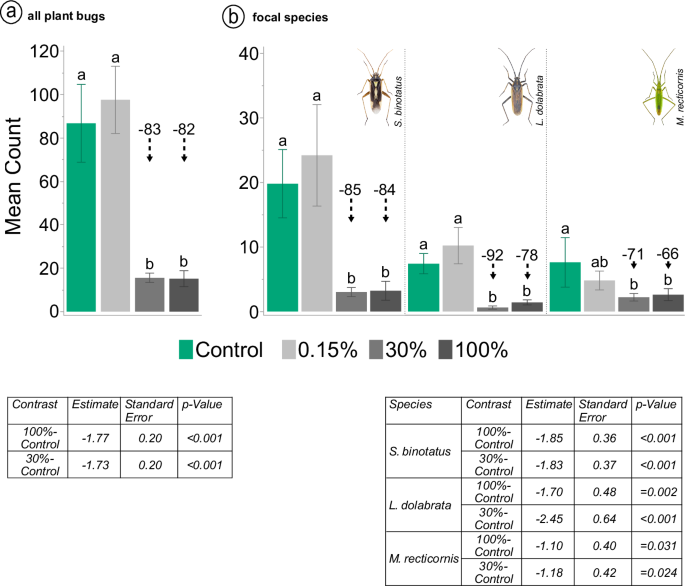
a Mean number of plant bug imagines and nymphs two days after insecticide application. Means not sharing the same letter are significantly different based on a Tukey test at the 5% level of significance following the generalised linear mixed model. Results for significant contrasts to the control are shown in the adjacent table. A detailed report is provided in Supplementary Table S1. Black dashed arrow lines in combination with numbers above bars indicate percentage difference to the control (rounded numbers). b Mean number of plant bug imagines two days after insecticide application separated by species. Stenotus binotatus (left), Leptopterna dolabrata (centre) and Megaloceroea recticornis (right). Means not sharing the same letter are significantly different based on a Tukey test at the 5% level of significance following the generalised linear mixed model. Results for significant contrasts to the control are shown in the adjacent table. A detailed report is provided in Supplementary Table S2. Black dashed arrow lines in combination with numbers above bars indicate percentage difference to the control (rounded numbers). N = 5 for all treatments and species (a, b). Error bars indicate standard error. Insect images © Gerhard Strauss, Biberach, Germany.
Focusing on the three most abundant species, the mean counts for S. binotatus, L. dolabrata and M. recticornis in the 30% and 100% treatment were significantly reduced compared to the control two days after insecticide application (S. b. 100%: p < 0.001, S. b. 30%: p < 0.001; L. d. 100%: p = 0.002; L. d. 30%: p < 0.001; M. r. 100%: p = 0.031; M. r. 30%: p = 0.024) (Fig. 2b). A detailed report of the contrasts is given in Supplementary Table S2. As with the total number of plant bugs, the proportions between treatments for these three species shifted at later sampling dates, probably due to a combination of repeated sampling and a decline in overall abundance due to the natural phenology of the species. While these factors probably affected counts at later samplings, the population dynamics shown in Fig. 3 suggest that there has been no recovery at high treatment doses (e.g. by recolonization).
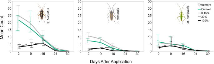
Population development of Stenotus binotatus (left), Leptopterna dolabrata (centre) and Megaloceroea recticornis (right). A solid green line indicates control treatment, a solid grey line indicates 0.15% Mospilan®SG treatment, a solid black line indicates 100% Mospilan®SG treatment, and the dashed grey line indicates 30% Mospilan®SG treatment. Curves are fitted with the Kernel method (local fit: linear). Points indicate mean number of imagines per treatment, and error bars indicate standard error of means. N = 5 for all treatments and samplings. Insect images © Gerhard Strauss, Biberach, Germany.
Pesticide analysis of vegetation samples from the enclosures (aboveground plant material including leaves, stems, and inflorescences of grasses and herbs) taken after 7, 17, and 30 days revealed residues of acetamiprid and its metabolite acetamiprid-N-desmethyl in the 100% and the 30% treatments (Table 1). No residues were found in the 0.15% treatment or in the control at any sampling time. Further information on pesticide analysis is provided in Supplementary Note 1.
Greenhouse experiment
Mospilan®SG reduced the survival for all plant bug species on plants sprayed with 30% of the field application rate (=75 g Mospilan®SG/ha in 600 l water) to mimic field-margin exposure 48 h ahead of plant bug release. Specifically, we observed a reduction of 88% for S. binotatus, 39% for L. dolabrata, and 35% for M. recticornis compared to the respective controls four days after transfer on contaminated plants (Fig. 4). Notably, no individuals of S. binotatus survived the insecticide treatment in any of the nine replicates.
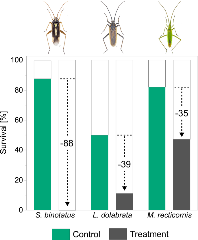
Plants were sprayed with insecticide two days prior to plant bug release. Survival rates at day four are given for Stenotus binotatus, Leptopterna dolabrata and Megaloceroea recticornis for the control (green) and the insecticide treatment (grey). Note that no individuals of S. binotatus survived the insecticide treatment and therefore no bar is shown. Black dashed lines in combination with numbers indicate percentage difference between survival in the control and treatment of the respective species. N = 9. Insect images©Gerhard Strauss, Biberach.
Acetamiprid and the metabolite acetamiprid-N-desmethyl were found in all samples collected from treated plants two days after application (i.e. the time of plant bug release). The mean concentration was 267 (±78) ng/g plant material for acetamiprid and 62 (±33) ng/g for acetamiprid-N-desmethyl (dry weight; N = 9; rounded numbers). Further information on pesticide analysis is provided in Supplementary Note 1.
Dose-response assays
All three species showed high sensitivity to the Mospilan®SG treatment in the topical dose-response assays in the laboratory (Fig. 5). Comparing the observed lethal doses required to kill 50% of individuals (LD50) for L. dolabrata (53.3 ng/µl), M. recticornis (39.0 ng/µl) and S. binotatus (4.1 ng/µl) with the typical field concentration of 416.0 ng/µl, the LD50 values for L.d. would correspond to 12.8%, M.r. 9.4% and S.b. 1.0% of the field concentration. In addition, pronounced species-specific differences were observed, with S. binotatus being significantly more sensitive to the insecticide than the other two species based on LD50 comparisons (L. dolabrata − S. binotatus: p = 0.001, t = 3.33; M. recticornis − S. binotatus: p = 0.021, t = 2.33).
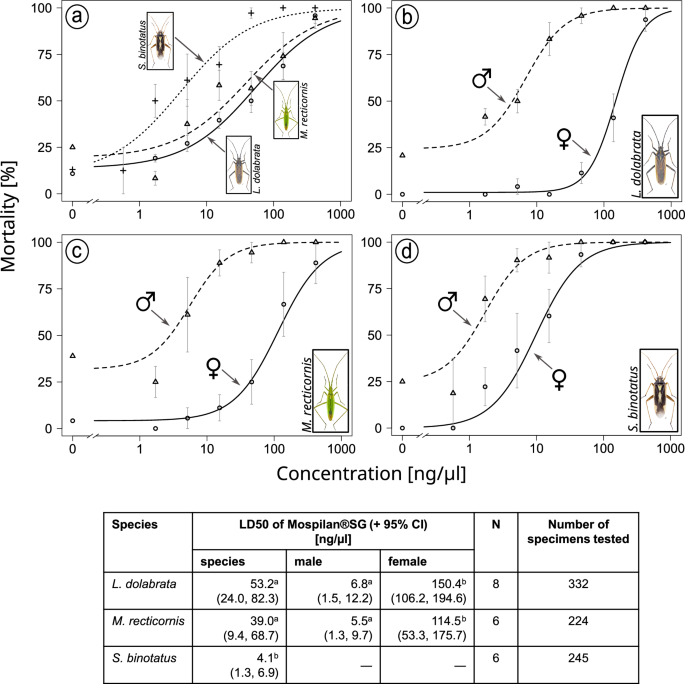
a Dose-response curves for all species, b separated by sex for Leptopterna dolabrata, c separated by sex for Megaloceroea recticornis, and d separated by sex for Stenotus binotatus. Data points represent mean values per concentration, with error bars indicating the respective standard error for all concentrations greater than zero. Note that mean values for the lowest Mospilan®SG treatment for males and females of M. r. consist of only four replicates instead of six. Insect images © Gerhard Strauss, Biberach, Germany. Derived LD50 values are shown in the table below. Separate LD50 values for male and female specimens were generated only for those species where sensitivity to the insecticide was significantly different between the sexes based on the fitted generalised linear mixed model (GLMM). LD50 values were compared using the compParm function of the ‘drc’ package in R. LD50 values of species not sharing a common letter are significantly different. LD50 values of males and females of the same species not sharing a common letter are significantly different. CI confidence interval, N number of biological replicates (i.e. Petri dishes) per concentration.
Besides the high toxicity of Mospilan®SG, we observed significant differences between males and females of two species. Based on LD50 values, males of L. dolabrata and M. recticornis were >20 times more susceptible than females (L. d. t = 6.33, p < 0.001; M. r. t = 3.48, p < 0.001). Sensitivity was not significantly different between the sexes of S. binotatus based on the fitted generalised linear mixed model (GLMM). Therefore, no LD50 values are reported from the dose-response model.
Discussion
Insecticides are considered a major cause of insect decline, but there is a lack of empirical evidence on the environmental effects on non-target species within and outside the cropping area. Using a neonicotinoid formulation, we studied the effect of terrestrial insecticide contamination on non-target plant bug communities. We conducted a series of field, greenhouse, and laboratory experiments to investigate community-, species- and sex-specific responses in this insect group. Plant bug species in the field experiment were highly sensitive to neonicotinoid exposure. We also found species-specific responses across different scales (i.e. field, greenhouse, and laboratory), and drastic differences in sensitivity between males and females.
Plant bug communities are highly sensitive to insecticide exposure
Consistent across experiments, our study shows a high susceptibility of plant bugs to insecticide exposure. In the field experiment, we aimed to simulate a scenario of overspray and direct drift contamination with specimens present in the off-field environment during spray application. A drastic reduction in plant bug abundance was observed in the scenario representing exposure within one metre of the field (30% of the typical field rate).
A second scenario of indirect drift contamination for the same field distance was simulated in the greenhouse experiment, as it is also possible that insects enter an area only after drift contamination occurs (i.e. after insecticides are applied). Residues of the compound that may still be present on surfaces (soil or plant material) hours or days later can still be absorbed through an insect’s cuticle, e.g. via the tarsi39, or ingested during feeding. In addition, in systemic insecticides such as neonicotinoids, the active ingredient can be taken up by plants, providing an additional route of oral exposure for piercing-sucking herbivorous insects (e.g. plant bugs) over extended periods of time. This is not surprising as systemic insecticides are specifically designed to protect crops by controlling pests in this way. However, this mechanism also inevitably affects non-target insects. In our experiment, even two days after host plants were treated with 30% of the typical field rate of Mospilan®SG, the survival rates of plant bugs placed on these plants were significantly reduced and even zero in S. binotatus.
These results clearly demonstrate the detrimental effect of insecticide contamination on non-target plant bug populations located close to arable fields. Further, a generally high sensitivity to neonicotinoid insecticides of this ecologically relevant insect group that most likely occupies an important position in the trophic pyramid, is revealed34,40. This pattern was further supported by the insecticide dose-response assays. Here, acute contact LD50 values for three plant bug species, simulating direct exposure from spraying, were at concentrations corresponding to 1% of the typical field concentration. To put our findings into a broader context, these values can be compared to those of common model organisms such as the Western honeybee A. mellifera. However, LD50 values from dose-response assays are typically given as a concentration of pure active ingredient per microliter or per individual. To establish comparability, the values we obtained using a commercial insecticide formulation can be adjusted to reflect the 20% active ingredient acetamiprid content. Based on the LD50 values reported in Fig. 5, this corresponds to 10.63 ng acetamiprid /bug for L. dolabrata, 7.81 ng/bug for M. recticornis and 0.82 ng/bug for S. binotatus. For honeybees, an LD50 of ~9260 ng active ingredient per bee is reported as contact exposure value, also based on a 20% acetamiprid formulation41. Accordingly, the sensitivity of the tested plant bug species is ~ 871 times (L. dolabrata) to ~ 11,293 times (S. binotatus) higher, which can be either explained by differences in species sensitivity or formulations. In general, several factors could cause differences in sensitivity between mirids and honeybees, such as body size, cuticle composition, body fat content, or the fact that the honeybee, as a dietary generalist, is potentially adapted to be exposed to a great variety of defensive secondary plant compounds (i.e. toxins) in nectar and pollen, whereas the plant bugs tested only feed on grasses.
However, comparisons between species involving different formulations should be made with caution. Nevertheless, the pronounced differences in LD50 values show that plant bugs are very sensitive to neonicotinoid insecticides and consequently to environmental contamination at only a fraction of the applied field concentrations. This is consistent with existing literature suggesting that plant bugs are usually very sensitive to neonicotinoid insecticides31,42,43. This group of insects should therefore be given greater consideration in risk assessment (see “Environmental risk assessment” below).
Species-specific sensitivity
The three plant bug species that were tested in this study can be considered representative non-target herbivorous insects. Specifically, these species are of particular interest because they share a similar ecology (e.g. feeding habits, phenology, and host plants28) and yet showed markedly different insecticide susceptibility under the experimental exposure scenarios. Differences in species response were already suggested by the field experiment and further confirmed by the greenhouse experiment with treated plants and the dose-response assays in the laboratory. Therefore, they clearly represent physiological differences between species and are not related to feeding preferences or position on the plant during spraying. The species differences are also unlikely to be explained by age differences due to different phenologies, as adult specimens of the three species appeared simultaneously in the field and had overlapping phenologies (see phenogram Supplementary Fig. S1).
Physiological factors that have been proposed to influence sensitivity include, for example, differences in the activity and abundance of detoxification enzymes, or simply body size44. Notably, the smallest (and lightest) species, S. binotatus, was always the most sensitive in our greenhouse and dose-response assays, suggesting that body size or mass may be an important factor. Consistent with this, Goulson45 compared neonicotinoid LD50 values reported in the literature and stated that much of the variation in sensitivity between different insect taxa could be explained by differences in body size or weight. For example, the pronounced difference in LD50 values between the plant hopper Nilaparvata lugens and the Colorado potato beetle Leptinotarsa decemlineata for the neonicotinoid imidacloprid was explained by body mass (~1 mg vs ~130 mg). Here we found, that although L. dolabrata has more than twice the body mass of M. recticornis, the LD50 values were almost identical when corrected for body mass (L. d.: 0.53 ng a.i./mg bug, M. r.: 0.66 ng a.i./mg bug; see Supplementary Tables S3 and S4). At the same time, the susceptibility of S. binotatus is still four times higher when corrected for body mass, suggesting either additional physiological factors or a non-linear relationship between body mass and susceptibility.
While the physiological mechanisms involved remain to be investigated, differences in species susceptibility could permanently alter local community structure under a constant or repeated exposure scenario. Changes in aquatic invertebrate community composition have been associated with pesticide contamination in the past21,46, whereas the effects on terrestrial invertebrate communities are less well explored. A recent meta-analysis showed that pesticide contamination reduces soil invertebrate diversity27 and studies on neonicotinoids show that they affect the abundance, diversity and community structure of soil invertebrates25,26. Also, Main et al.47 linked neonicotinoid soil contamination to reduced wild bee species richness in field margins. However, especially for insect herbivores, which play a central role in terrestrial food webs48, more research is needed to understand the consequences of pesticide exposure at the landscape scale. Particular attention should be paid to univoltine species with short nymphal and adult phenologies that may overlap with common pesticide application regimes such as the plant bugs studied here.
Sex-specific sensitivity
In addition to differences in sensitivity at the species level, we found that males of L. dolabrata and M. recticornis were significantly more sensitive to the insecticide than the corresponding females. Sex-specific insecticide sensitivity is a pattern reported for many insects, with males often being more susceptible than females49,50. However, there are also contrary reports in some species51.
Potential factors involved in sex-specific susceptibility partly overlap with those likely driving the observed species-specific differences. The most likely factor is again body mass, especially in sexually dimorphic species such as L. dolabrata and M. recticornis. In both species, males had a lower mean fresh body mass than females, with a 2.9-fold difference in L. dolabrata and a 2.2-fold difference in M. recticornis (N = 10 per species and sex). This is not directly reflected in the difference in LD50 values between males and females, which is 22-fold for L. dolabrata and 21-fold for M. recticornis. However, as mentioned above, such relationships may not be necessarily linear.
Another source for differential susceptibility is at the enzymatic level. Frohlich52 showed that the activity of detoxification enzymes decreased with age in males of the solitary bee Megachile rotunda, but not in females. An age-dependent change in enzyme activity was also observed by Guirgus and Brindley53 when they compared 1-day-old males of Megachile pacifica with 4-day-old males, both of which had been previously treated with a fungicide. Thus, age also appears to play a critical role in the susceptibility of insects to insecticides.
The higher control mortality observed in males in our dose-response study (which was considered in the models) could suggest an older initial age compared to females in the same cohort. Wheeler34 noted that in most plant bug species, males usually appear before females and do not live as long. In addition, for L. dolabrata, Wachmann et al.28 suggest that females live longer than males. A lower vitality of male specimens due to a shorter life cycle (i.e. a higher relative age at the time of sampling) could therefore explain a higher mortality in the controls and therefore a higher susceptibility to stressors such as insecticides. Tan et al.54 have previously suggested that imidacloprid disproportionately affects males of the plant bug Apolygus lucorum beyond the sex differences observed in controls. However, in all three species, the interaction between ‘cohort’ and ‘sex’ did not explain any variance in the data when tested in the GLMM (see “Methods”). Therefore, in our dose-response assays, the age of the sampled field population (=cohort) is unlikely to influence the differential insecticide susceptibility between males and females.
Regardless of the underlying mechanisms, the observed differences of a full order of magnitude could lead to a shift in sex ratios, in this case towards females. This could ultimately lead to a reduction in abundance and, in the long term, a shift in species composition.
Environmental risk assessment
To assess the risk of insecticide contamination to non-target species, it is essential to determine the true vulnerability of these species in their natural environment. Vulnerability involves both physiological sensitivity and exposure to an insecticide55. We have shown that plant bugs, as a non-target group, are physiologically highly sensitive to insecticides. Furthermore, the species tested here are likely to occur in highly exposed areas of the off-field environment, i.e. grass-dominated field margins or adjacent meadows28. We also demonstrated that exposure to a systemic insecticide extends beyond the initial contamination by direct contact with spray droplets, as plant bugs placed on previously sprayed plants showed a drastic reduction in survival. Considering that in the field experiment, we were able to detect acetamiprid in host plant tissue up to 30 days after application, the threat to non-target plant bugs is long-lasting. It is therefore all the more surprising that the current risk assessment does not consider this group or other herbivorous insects in the non-target insect community. In addition, field margins less than 3 m wide are currently not considered to be terrestrial non-target habitats for pesticide application in Germany56. Consequently, this habitat and the insects living there are not protected from pesticide contamination13.
Roß-Nickoll et al.57 argue that the test procedures used in the EU risk assessment are insufficient because the test species used do not adequately reflect the non-target insect community. As a result, the disruption to these communities caused by pesticide exposure is not considered. This discrepancy is further illustrated by the drastic difference in LD50 values between the honeybee model and the mirid species we tested, suggesting up to ~ 11,000 times higher toxicity to plant bugs compared to the honeybee. In addition, risk assessment is currently only done at the species level, and sex-specific sensitivity is not considered. However, the up to 22-fold difference in LD50 values between sexes that we found could scale to detrimental long-term effects on plant bug community composition. This calls for an increase of the so-called uncertainty factors used to cover different species and sexes from currently 10 to at least 1000 (based on the least sensitive species, L. dolabrata). Consequently, and in light of the renewal of the authorisation of acetamiprid until 203358, we argue that the current European risk assessment system urgently needs to be adapted accordingly to adequately address the environmental risk of pesticide contamination.
Methods
Statistical analysis and graphical representation
Statistical analysis was conducted using R59 (version 4.3.0) and R-Studio60 (version 2023.6.1.524). Additionally used R-packages are cited in the following sections.
All graphs showing bar or stacked bar charts were generated using JMP®Pro61 (version 17.2.0). Dose-response curves were generated with R using the package ‘drc’62. All figures were processed with Inkscape63 (version 1.3.2).
Field experiment
Construction
In May 2022, we established 20 field enclosures (2 m × 4 m) on an extensively managed meadow (48°42’31“N 9°12’48“E) in the botanical garden of the University of Hohenheim, Stuttgart, Germany. In every corner of each enclosure, a 1.4 m long wooden pole was vertically inserted 40 cm into the soil. An 85 cm high insect gauze (mesh size: 0.27 mm x 0.79 mm, Howitec Netting bv, AH Joure, the Netherlands) was vertically stretched around these poles. About 10 cm of the gauze was inserted into the ground to form a barrier, while 75 cm was left above ground attached to the poles. This left the top of the field enclosure uncovered. These semi-open field enclosures were additionally reinforced with tent cords that were attached at each corner. On an area of 340 m2, we set up 20 enclosures in seven rows, each one 2 m away from its neighbour on all sides. The field experiment was laid out as a randomized block design with four treatments: three different concentrations of insecticide and a control. Each enclosure was defined as an individual replicate with every treatment being replicated five times (Fig. 1). The choice of blocks was made with respect to the environmental conditions on the site. Due to surrounding trees, the duration of direct sunshine was longest in the north-western area and shortest in the south-eastern area. In addition, the test site was located on a south-facing slope. This resulted in a soil moisture gradient towards the south slope. The following blocks were assigned accordingly: A = upper slope + high sunshine duration, B = middle slope + high sunshine duration, C = middle slope + medium sunshine duration, D = lower slope + medium sunshine duration, E = lower slope + low sunshine duration (see Supplementary Fig. S2).
Insecticide application
We used the nerve-acting neonicotinoid insecticide Mospilan®SG, with the active ingredient acetamiprid (CAS 135410-20-7) for all experiments described in this study. The following concentrations were applied by spraying in the field experiment: (1) typical field application rate for e.g. potatoes, cabbage, lettuce or beetroot of 250 g/ha in 600 l of water (100%), (2) 30% of the field application rate, and (3) 0.15% of the field application rate. These values are based on estimates for overspray- and drift contamination at different field distances9,37. The underlying concept is illustrated in Fig. 1b. In the control, only tap water was applied. The application rate was scaled down to the field plot area of eight square metres (Table 2). The amount of 0.48 l containing the respective insecticide concentration was applied equally to each field enclosure using the GLORIA prima 3 hand sprayer (GLORIA Haus- & Gartengeräte GmbH, Witten, Germany).
The hand compression sprayer was calibrated before use and the volume output was measured. The mean deviation of liquid output was around 1%. Details of the calibration procedure are given in Supplementary Note 2.
The application started with the control (water only) followed by the insecticide treatments in increasing concentration. Between treatments, the hand sprayer was completely emptied and re-calibrated. To control for uneven application due to a change in volumetric flow rate (because of decreasing pressure during spraying), the field plots were divided into four equal quarters. Each quarter was assigned a number from one to four. Spraying would always start in the quarter numbered one and end in the quarter numbered four. The order of numbers was randomized within plots of the same treatment.
During application inside the enclosures, the spray gun was opened with the nozzle pointing downwards towards the soil while moving in a standardized pattern of vertical and horizontal trajectories at a height of 80 cm above the ground. This was done for 21 s per quarter (1/4 of 84 s being the total application time per enclosure) and then repeated for the other quarters of the same field enclosure. To prevent contamination of surrounding enclosures, each enclosure was surrounded by a 2 m high plastic sheet during application.
Exposure analysis
Seven days after insecticide application, vegetation samples were collected from inside the field plots to quantify the amounts of the active ingredient acetamiprid and the metabolite acetamiprid-N-desmethyl by LC-MS analysis. This was done to verify the potential presence of the insecticide inside the enclosures according to the different treatments even days after application, as well as its metabolization within the plant tissue. Composite vegetation samples were collected from the interior of all plots at 7-, 17-, 30-, and 60-days after insecticide application and stored at −20 °C. Two grams of randomly selected frozen material (fresh weight) were crushed with liquid nitrogen in a mortar and transferred to a 100 ml centrifuge tube. Acetonitrile (ACN; 20 ml) and 250 µl distilled water were added, and the mixture was homogenized for 1 min using a Miccra MiniBatch D-9 (MICCRA GmbH, Heitersheim, Germany). The sample was filtered into a 25 ml volumetric flask and brought to a total volume of 25 ml with ACN. Two millilitres of the mixture were transferred to a 2 ml Eppendorf tube, and 20 µl ethylene glycol was added. The extracts were reduced to 200 µl at 60 °C under nitrogen flow in a Vapotherm mobil S (Barkey GmbH & Co KG, Leopoldshöhe, Germany), then adjusted to 0.5 ml with a 3:7 ACN/water mixture and centrifuged at 12,000 rpm for 10 min (miniSpin, Eppendorf AG, Hamburg, Germany). The supernatant was transferred to auto sampler glass vials using a syringe with a 0.45 µm PTFE filter (ROTILABO® Mini-Tip, Carl Roth GmbH + Co. KG, Karlsruhe, Germany). For quantifying acetamiprid and its metabolite, 3 µl of the extract was injected into an LTQ Velos LC-MS system (Thermo Fisher Scientific, Waltham, Massachusetts, USA). Compounds were separated on a Kinetex® 2.6 µm XB-C18 LC column (Phenomenex Ltd. Deutschland, Aschaffenburg, Germany) at 40 °C and a flow rate of 0.5 ml/min using the following water + 10% ACN (A)—ACN (B) gradient: 0–1 min 95% A, 10 min 40% A, 12–14 min 10% A, and 14.1–16 min 95% A. Quantification was carried out using a calibration curve (0.005, 0.01, and 0.1 mg/l). To determine the amount of compound per gram of plant tissue, the dry weight of a 2 g sample was determined for each sample after drying at 80 °C for 24 h in a Heraeus T12 oven (Heraeus Instruments, Hanau, Germany). The full analytical procedure and results are given in Supplementary Note 1.
Insect sampling and identification
Insects in the upper vegetation of each field enclosure were regularly sampled with a sweep net (Flexi-Kescher Dreieck; Bioform, Nuremberg, Germany). Sampling took place 2, 9, 16, 24 and 30 days after insecticide application. While walking parallel to the enclosure, the net was swept four times forward and backward across the upper part of the vegetation. After the fourth sweep, the net was immediately closed by hand. The entire contents were then transferred into a three-litre zip-lock plastic bag (Profissimo, dm-drogerie markt GmbH+ Co. KG, Karlsruhe, Germany). The plastic bags were stored at −20 °C for at least 24 h to kill all arthropods inside.
For evaluation, individual bags were stored at 8 °C for 30 min to carefully unfreeze the specimens. The entire contents of the plastic bag were then transferred to a plastic tray and the plant bugs (imagines and nymphs) were separated with tweezers. Nymphs were counted and transferred to a 2 ml screw-capped microtube (SARSTED AG & Co. KG, Numbrecht, Germany) filled with 70% ethanol (and 30% tap water) for preservation. Imagines were sorted into morphospecies, and individuals were counted. For each morphospecies, one male and one female specimen (if available) were separated for preparation. The specimens were mounted on paper cards using wallpaper glue. In the case of male specimens, the aedeagi were removed beforehand and glued next to the respective specimen. The remaining specimens were preserved in 70% ethanol (and 30% tap water) as described above. All morphospecies were identified to species level using the Hackston64 Miridae key and the Corisa software65.
Statistical evaluation
A generalised linear mixed model (GLMM) was fitted for the combined individual counts of nymphal and adult plant bugs using the ‘lme4’ package (version 1.1-3366) with ‘count’ as the explanatory variable, ‘treatment’ as a fixed effect, ‘sampling’ as a co-factor, and ‘block’ and ‘plot’ (=enclosure ID) as random effects assuming a Poisson distribution. An interaction between treatment and sampling was included. The fixed effect ‘treatment’ was modelled categorically as we only wanted to compare means between treatment groups. In addition, ‘treatment’ consists of only a small number of steps, which are also very irregularly spaced (0%, 0.15%, 30%, and 100%). Identifying a suitable non-linear model is therefore difficult and was not attempted. Model fit was assessed by residual analysis, considering the R2 value and the Akaike Information Criterion (AIC), and by checking for possible over-dispersion. Significant factors and interactions within the model were identified using a post-model ANOVA. Those were ‘treatment’, ‘sampling’ (i.e. time of sampling after application) and the interaction between both factors. Pairwise post hoc multiple comparisons by sampling were then executed using the Tukey test based on estimated marginal means using the emmeans package67 considering the treatment–sampling interaction.
In a second step, a separate GLMM was fitted including only the count data of adult S. binotatus, L. dolabrata and M. recticornis specimens and only the data of the first sampling (i.e. two days after insecticide application). In this GLMM, ‘count’ was the explanatory variable with ‘treatment’ as a fixed effect, ‘species’ as a co-factor, an interaction between ‘treatment’ and ‘species’ and ‘block’ and ‘plot’ as random effects, assuming a Poisson distribution. Model fit was assessed as described above. Significant factors and interactions within the model were identified using a post-model ANOVA. Pairwise post hoc multiple comparisons by species were then executed using the Tukey test based on estimated marginal means considering the treatment–species interaction.
Based on the control sampling data of the three species, the populations were stable in the early samples, but declined dramatically in later samples as expected based on the known phenologies. To compare acute species-specific treatment response, we therefore did not include data beyond the first sampling. The full R-code is provided in Supplementary Codes 1 and 2.
Greenhouse experiment
Host plant preparation
Eighteen plots of 30 cm diameter with live plants, consisting mainly of grasses, which are the host plants of the three mirid species included in this experiment (see next paragraph), were collected from a meadow with a shovel and transferred to 12-l plant pots. These were previously filled halfway with a 50:50 mixture of sand and humus. Only sections of the meadow with a high proportion of grasses were selected to provide sufficient host plants for the plant bugs. The pots were placed in an outdoor test facility for one month and watered as needed until the grasses had developed seed heads.
Insecticide application and experimental procedure
The pots were placed in an 8 m2 rectangular area, surrounded by 2 m high vertical plastic sheathing. Spray application was carried out using the same protocol and equipment as described for the field experiment. Two treatments were applied: a solution containing a 30% field rate concentration of Mospilan®SG (75 g/ha in 600 l water, see Table 2) and a control containing only water. For each treatment application, nine randomly selected plant pots were placed within the application area, all 30 cm apart. The full 8 m2 was either sprayed with water (control) or the 30% Mospilan®SG solution. The control was applied first. The pots were then placed in the outdoor test facility. A total of four blocks were formed, with two blocks for each treatment, one containing five pots and the other one containing four. Treatment and control blocks with the same number of replicates were placed opposite to each other (Fig. 6). In the centre of each pot, a 2 m wooden stick was vertically inserted. At the top of the stick, a 30 cm diameter wire ring was fixed horizontally. Fine insect gauze was then placed over the construction from the top of the stick down to the plant pot, forming a closed tube around the host plants.
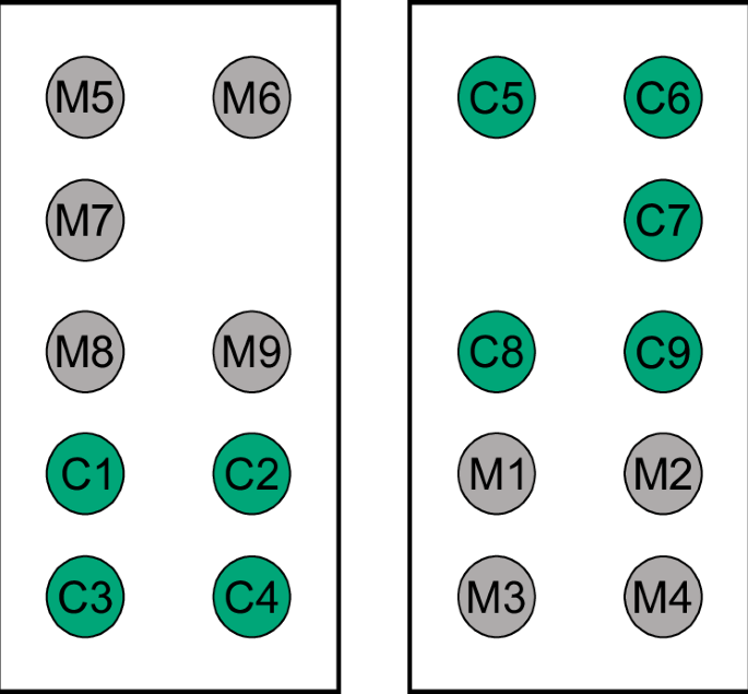
Treatment and control blocks with the same number of replicates are placed opposite to each other. M Mospilan®SG treatment (green), C control treatment (grey), numbers indicate replicate ID.
Two days after application, plant bugs were caught using a sweep net (Flexi-Kescher Dreieck; Bioform, Nuremberg, Germany) in the same extensively managed meadow from which the plant samples were collected. Specimens were immediately transferred to 30 cm × 30 cm AERARIUM mesh cages (Bioform, Nuremberg, Germany), which were then placed in an 8 °C room. After 15 min of settling, the cages were opened and specimens of S. binotatus, L. dolabrata and M. recticornis were sorted by species (identified by the naked eye) and transferred to petri dishes. For each replicate (=one plant pot), three Petri dishes were prepared, each containing six specimens of either species (males and females mixed). After assuring that all bugs were vital, 18 plant bugs (6 per species) were released on top of the plants inside the insect gauze. At the same time, plant samples for HPLC analysis were collected from each Mospilan®SG treated pot to demonstrate that the active ingredient acetamiprid was present at the time of plant bug release. Each morning the plants were sprayed with a plant sprayer to simulate morning dew. After four days (six days after insecticide application) the experiment was terminated, and alive specimens were counted. Specimens from each replicate were stored separately in 2 ml microtubes with screw caps (SARSTEDT AG & Co. KG, Germany) filled with 70% ethanol (and 30% tap water). Following the assay, species identity was again verified using a binocular, the Hackston64 Miridae key and the Corisa software65.
Exposure analysis
Two days after the insecticide application, just before the plant bugs were released into the cages, vegetation samples were collected from each replicate of the insecticide treatment group. Unlike the field experiment, the control group was not sampled as the control pots were sprayed first and then removed before insecticide application. LC-MS analysis was used to quantify the amounts of the active ingredient acetamiprid and the metabolite acetamiprid-N-desmethyl as described in the field experiment. The full analytical procedure and results are provided in Supplementary Note 1.
Statistical evaluation
A linear mixed regression model was fitted using the ‘lme4’ package66 with ‘alive’-specimens as the response variable, ‘treatment’ as a fixed effect and ‘species’ as a co-factor, and an interaction between ‘treatment’ and ‘species’. The random factor ‘block’ was first included but did not explain any variance of the data and was therefore excluded from the model. The random factor ‘pot’, providing a unique identifier for each pot, was included to account for the fact that ‘species’ was nested within ‘treatment’, allowing individual baseline mortality for each replicate. Hence, if the interaction was significant, it was not due to a replicate effect, allowing to explore species differences in survival only. The significant interaction between ‘treatment’ and ‘species’ was confirmed by an ANOVA.
Fitting a follow-up model with ‘species’ as the explanatory variable was not possible because there were no individuals of S. binotatus that survived the insecticide treatment in any of the nine replicates, making it impossible to estimate a standard error. Accordingly, we report the difference in treatment effect as the percentage difference in survival rates between the control and insecticide treatments (‘insecticide effect’). This considers the baseline mortality of each species observed in the control. The full R-code is provided in Supplementary Code 3.
Dose-response assays
Insecticide preparation
A stock solution of 4.16 mg/ml Mospilan®SG, dissolved in tap water, was prepared corresponding to ten times the highest recommended field rate of 0.416 mg/ml. Stock and treatment solutions were stored in 1.5 ml ND8 amber glass screw-neck vials (LABSOLUTE—TH GEYER) in the dark at 4 °C. Stock solutions were freshly prepared every week. Prior to each dose-response assay, a dilution series was prepared based on the stock solution on the day of application (Table 3).
Here, 0.5% TWEEN® 20 was added to the solvent to break the surface tension and facilitate spreading on the bug’s body surface. Each treatment concentration was prepared from the stock solution by pipetting volumes from higher to lower concentration treatment tubes prefilled with pure solvent (see dilution protocol Supplementary Note 3). The Tween® 20 solvent was also applied to the bugs in the control group.
Insect sampling
Plant bugs were collected as described in the greenhouse experiment. Two Petri dishes were prepared per species and treatment with six to four specimens each (depending on the availability of specimens). Where possible, male and female specimens were equally distributed. Only vital specimens that were actively climbing the net were included. Petri dishes were taken to the laboratory (20 °C) where the specimens were allowed to settle again for 20 min. Prior to treatment application, all specimens were again checked for vitality and replaced if necessary.
Topical application and evaluation
Several identical assays were run in sequence to control for a possible cohort effect (S. binotatus + M. recticornis: three assays; L. dolabrata: four assays). Each assay included two replicates per concentration (i.e. Petri dishes), each consisting of four to six specimens (typically 2 males + 2 females/3 males + 3 females) based on the availability of specimens. After the treatment, all specimens of one replicate were first placed in a new petri dish and later transferred to plastic cups (see below). Accordingly, each concentration consisted of six- (S. b. + M. r.) or eight replicates (L. d.) nested within three or four cohorts (Table 4). Note that for M. recticornis the number of replicates in the lowest tested Mospilan®SG concentration (0.41%) is four instead of six.
The number of treatments for S. binotatus was increased for the second and third cohort adding the 0.14% treatment due to the observed higher sensitivity of this species.
Bugs inside Petri dishes were anaesthetized with CO2, and then 1 µl of insecticide solution (or pure solvent as a control) was applied dorsally to each specimen. The application was conducted using the Hamilton repeating dispenser with a 50 µl Hamilton syringe (Hamilton Bonaduz AG, Switzerland). Specimens of each replicate were then transferred to 500 ml plastic cups. The cups contained a water supply (Eppendorf tubes filled with water and cotton wool), a bundle of grasses from the original habitat with the top 10–15 cm of the plants cut off (stems and heads) placed in an Eppendorf tube filled with water and cotton wool, and a paper tissue covering the bottom of the cup. Several holes have been made in the lid to allow for air exchange. In addition, water was sprayed once into the cup to cover the grasses with droplets providing sufficient humidity and an additional source of drinking water. Cups were stored under standard laboratory conditions. After 24 h, mortality rates for all treatments were recorded for each replicate and sex. The experiment was then terminated and dead and surviving specimens from each replicate were stored separately in 2 ml microtubes with screw caps (SARSTEDT AG & Co. KG, Germany) filled with 70% ethanol. Following the assay, species identity and sex of all specimens were again verified using a binocular, the Hackston64 Miridae key and the Corisa software65.
Dose-response analysis
Data from each assay were first analysed with a generalized linear mixed model using the ‘lme4’ package66. ‘Mortality’ was included as the explanatory variable, ‘concentration’ as a fixed effect, ‘sex’ as a co-factor and ‘replicate’ and ‘cohort’ as random effects. Additionally, an interaction between ‘concentration’ and ‘sex’ was included. An interaction between cohort and sex was also initially included to control for the possibility that the age of bugs collected in the field (=cohort) might influence treatment response with respect to sex. However, this interaction did not explain any variance in any of the species and was therefore excluded from the model. Model fit was assessed by residual analysis, considering the R2- and AIC value, and by checking for possible over-dispersion. Including the random effect ‘replicate’ allowed to control for the fact that ‘sex’ was nested within ‘concentration’, allowing an individual baseline mortality for each replicate. If the interaction was significant, it was not due to a replicate effect, allowing to generate LD50 values for male and female specimens of the same species separately.
A post-model ANOVA was performed confirming that ‘concentration’ was a significant predictor in all assays. A significant interaction between ‘concentration’ and ‘sex’ was found for L. dolabrata and M. recticonis.
Log-logistic dose-response models were then fitted for a combined species analysis and for each species while modelling male and female response separately using the ‘drc’ package62. To improve model fit, the lower asymptote of the fitted regression curve was not set to ‘0’ in order to generate unbiased parameter estimates in the presence of control mortality. The upper asymptote was set to ‘1’. The best model fit was selected based on visual inspection of the regression line and evaluation of the confidence intervals of the model parameters, considering the AIC estimator. Dose-response curves were generated using the plot() operation. LD50 values were obtained using the ED() function, including a control for possible over-dispersion of the logistic regression model. Differences between LD50 values of individual curves within the same model were analysed using the compParm() function executing approximate t-tests with α = 0.05 and including a correction for possible over-dispersion of the underlying model.
The full R-code is provided in Supplementary Codes 4 and 5.
Documentation of notification regarding the mentioned product Mospilan®SG
The registration holder and the producer of Mospilan®SG were informed of the forthcoming publication and its content prior to the publication of this study and were allowed to comment. The companies concerned did not respond within the prescribed time limit of five working days and only referred to official sources of information in the field of plant protection products.
Reporting summary
Further information on research design is available in the Nature Portfolio Reporting Summary linked to this article.


Responses