The severe 2020 coral bleaching event in the tropical Atlantic linked to marine heatwaves

Introduction
Marine heatwaves (MHWs) are analogues to atmospheric heatwaves and have devastating impacts on marine ecosystems, ranging from habitat shifts and changes in population structure to mass mortality events of various marine species1. These extreme events can thus overwhelm the capacity of both natural and human systems to cope, causing socioeconomic impacts such as loss of essential ecosystem services and fisheries income2. The frequency and severity of MHWs have increased over the last century mainly due to anthropogenic climate change3,4,5 and will continue to do so as global temperatures continue to rise unabated4,6 with widespread consequences for marine ecosystems globally.
To guide adaptation and mitigation policies to avert the most severe impacts on marine ecosystems, it is essential to improve the understanding of the physical drivers of MHWs to improve their predictability7. Many studies in the last decade have revealed that MHWs can be forced by atmospheric and oceanic processes depending on the location and seasonality7,8. For instance, a large proportion of the most extreme extra-tropical MHW events are driven by persistent high-pressure systems and weaker winds that lead to increased insolation and reduced ocean heat losses9. This mechanism was responsible for several unprecedented events, including those in the Mediterranean Sea during the summer of 200310, in the northwest Atlantic in 201211 and in the southwest Atlantic during the austral summer of 2013/1412. MHWs can also be generated by increased ocean transport of heat, such as the event off western Australia in 201113 and reduced coastal upwelling in the case of the event off the Peruvian coast in 201714. A combination of multiple interacting mechanisms can also lead to extreme MHWs, such as the notorious North Pacific Blob15. Despite the emerging literature on the subject, very little is known about MHWs in the tropical Atlantic.
While their characteristics and drivers vary considerably, most MHWs have a common aspect – their negative impacts on the marine ecosystem. They affect foundation species such as corals, seagrasses and kelps1,16. The increase in MHW days observed in the last decades is associated with a decline in seagrass density and kelp biomass. Most relevantly, MHWs break the symbiotic relationship between hard corals and single-celled dinoflagellates (Symbiodiniaceae), leading to coral bleaching17. The impacts from acute events of MHWs on coral are more devastating than those from less severe long-lived MHW events. This is particularly true for corals that are typically categorised as thermally tolerant during milder events but can go under widespread bleaching and mortality as a result of an MHW event. Corals in the western tropical and South Atlantic, for instance, tend to be less susceptible to bleaching with low mortality and have suffered from 50% to 60% fewer mass bleaching events in comparison to the Indo-Pacific and the Caribbean18. Even though coral bleaching has been recorded recently in the tropical and subtropical South Atlantic19,20,21,22,23, there is relatively low mortality of dominant species when compared to bleaching events in the Indo-Pacific and the Caribbean24, with only more significant mortality occurring in branching hydrocorals (Millepora alcicornis) and the endemic coral (Mussismilia hartti) in the tropical Atlantic19,22,23. Projections indicate that the western side of the tropical Atlantic will be the most vulnerable area for bleaching25, threatening the most diverse reefs in the tropical Atlantic, such as the Abrolhos Bank reefs at 17°S25. These projections might be underestimating the potential threat to corals in the tropical Atlantic because they do not account for a higher frequency and severity of MHWs.
There is still a lack of knowledge of the impacts of MHWs on many species and populations, which limits our capacity to protect marine ecosystems from future extreme events. This is particularly the case for coral bleaching in nutrient-poor regions such as tropical waters. Even though a few studies investigate the drivers of MHWs in the tropical Indian and Pacific oceans14,26, none has focused on the tropical Atlantic. Thus, the objective of this study is to understand the physical drivers of MHWs in the western Tropical Atlantic that led to a severe coral bleaching event off the northeast coast of Brazil in the austral summer and fall of 2020. Here, we show that MHWs are becoming more frequent and intense in this region and that the summer/fall of 2020 was unprecedented for the historical record (1982–2022), resulting in a mass coral bleaching event.
Results and discussion
Marine heatwaves in the western Tropical Atlantic
To fill in the gap of knowledge of extreme temperature events in the tropical Atlantic, we analyse the spatial pattern and temporal evolution of the MHWs in the tropical Atlantic from 1982 to 2022 in the context of changes in sea surface temperature (SST). As expected, the all-time (1982–2022) mean SST along the tropical Atlantic between 7°N-15°S and 60°W-20°E presents a zonal gradient with the highest SST in the west and lowest SST in the east of the basin (shading in Fig. 1a). This is a response to the prevailing easterly trade winds (vectors in Fig. 1a) that push warm surface waters to the west and upwell cold waters to the surface in the east27.

a Sea surface temperature (shading; in °C) and wind at 850 hPa (vectors; in m s-1) averaged over the period 1982–2022. b Marine heatwave cumulative intensity (shading; in ˚C-day) averaged over the period 1982–2022 and wind anomalies at 850 hPa averaged during marine heatwave events (vectors; in m s-1). c Linear trend of sea surface temperature (shading; in °C per decade) and wind at 850 hPa (vectors; in m s-1 per decade). d Linear trends of marine heatwave cumulative intensity (shading; in °C-day per decade) and wind anomalies at 850 hPa for marine heatwave events (vectors; in m s-1 per decade). e Time series of monthly marine heatwave cumulative intensity averaged over the region between 7°N-15°S and 60°W-20°E (grey bars; °C-day) and monthly spatial extension of marine heatwaves within the same region (red line, in %). Dark grey contours in panels (c) and (d) encompass the areas where the trend is statistically significant at the 95% confidence level, majoritarianly in the basin’s western side.
In contrast, the all-time MHW cumulative intensity follows an opposite pattern, with the highest values to the east and lower values to the west (shading in Fig. 1b). This is because the MHWs are associated with a weakening of the trade winds over the region (vectors in Fig. 1b), allowing the warm waters from the west to flow eastward while decreasing the equatorial upwelling in the eastern side of the basin. In addition, weaker trades lead to a reduction of the heat flux from the ocean to the atmosphere, mainly due to less evaporative cooling28, as we shall see in the next section.
Analysis of the linear trends during 1982–2022 shows that the most significant changes in SST occur off the coast of Africa with no apparent long-term change in the winds (Fig. 1c). In contrast, the higher trends in the extremes (MHW cumulative intensity) occur in the western side of the basin (Fig. 1d), where the mean SST is already at its highest (Fig. 1a). This is particularly impactful for regional marine ecosystems. Considering that marine species with the smallest thermal safety margins are found near the equator29,30, finding the highest trend where the mean SST is already at its highest along the equator means there is a great chance of the SST passing the heat tolerance limit of many species. Regarding the winds associated with MHWs, there is a significant long-term weakening of the trades located over the area of maximum trends in MHW cumulative intensity along the equator.
A closer look at the time evolution of MHW cumulative intensity averaged over this region shows that there has been an increase not only in MHW cumulative intensity but also in the spatial extent of the MHWs in the tropical Atlantic (Fig. 1e). Moreover, the increase in cumulative intensity is related to the rise in frequency (numbers of MHW days, Fig. S1a) and intensity (amplitude of the SST anomalies during MHW days, Figure S1b). Ranking the most severe MHW summer/fall events shows that during the austral summer and fall of 2020, an unprecedented sequence of MHW events expanded over approximately 60% of the tropical Atlantic, with monthly MHW cumulative intensity averaging 22 °C-days (Tab. S1 and Fig. S2).
The geographical extent and persistence of the warming during the 2020 MHW events can be seen in Fig. 2. The MHWs develop in November (not shown) and peak in December and January over the southeastern and central equatorial Atlantic (Fig. 2a, b). By February, the MHWs ease over the eastern and central Atlantic and reach their peak in March over the western side of the basin (Fig. 2c, d). The MHWs weaken in April in most of the tropical Atlantic, disappearing in May in the equatorial eastern side (Fig. 2e, f). Note that computing the MHWs characteristics over a smaller area in the western tropical Atlantic (0°–7°S and 25°–35°W) does not change the results (Fig. S3). This is because the 2020 MHW events were so widespread in the tropical Atlantic that it is the most severe summer/fall on record, regardless of the selected area. Noteworthy to mention that the second and third most severe summer/fall MHWs occurred in 2019 and 2010, respectively (Tab. S1).
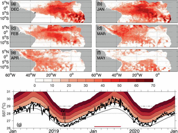
Mean marine heatwave cumulative intensity (shading; in °C-day) for: a December 2019, b January 2020, c February 2020, d March 2020, e April 2020, f May 2020. g Time series of observed SST (thick line), the long-term climatology (dotted line) and the 90th percentile climatology (dashed line) at Rio do Fogo reefs (5.2°S and 35.2°W; black star in panel a). Marine heatwave severity categories I–IV are shown in shades of red: I, moderate; II, strong; III, severe; IV, extreme. The grey dotted line represents the maximum monthly mean SST and the grey dashed line represents the bleaching threshold according to the NOAA Coral Bleaching Watch.
As we shall see, the sequence of MHW events in 2020 caused a massive coral bleaching off the northeast coast of Brazil22, including at the Rio do Fogo reefs we monitored (star in Fig. 2a). At this location, the waters are the warmest between January and April (dotted line in Fig. 2g). The SST was above the climatological mean for the whole period between January 2020 and April 2020 and surpassed the 90th percentile in 90 days out of a total of 120 days for the same period (solid, dotted and dashed lines in Fig. 2g, respectively). These extreme days comprised 5 MHW events of 32, 19, 11, 19 and 9 days of duration (Figure S4), categorised from moderate to strong events according to the methodology by Hobday et al.31. Moreover, they represent 30% of all January-April MHW days for the period of 1982-2020. We also compute the number of MHW days in which SST is above the threshold of 29°C, 29.5 °C and 30 °C (Fig. S5). If the SST surpasses these thresholds, the location represents a coral bleaching hot spot, according to NOAA Coral Bleaching Watch (more details in the Data and Methods). There was a total of 234 days in which the SST was above 29 °C for the period of 1982–2020, 33% of those occurred in January-April 2020 ( ≈ 76 days); for the threshold of 29.5 °C, 38% of the days in the record occurred in January-April 2020 ( ≈ 43 days) and 50% above 30 °C ( ≈ 12 days). In the latter case, this location experienced 12 consecutive days of SST above 30 °C in 2020. Before we discuss the biological impacts of this unprecedented summer/fall, we will investigate their physical drivers.
Drivers of marine heatwaves in the western tropical Atlantic
Now we turn our attention to the drivers of the most severe MHWs in the summer/fall of 2020, comparing with 2019 and 2010. As mentioned before, SSTs in the western tropical Atlantic are driven by surface heat fluxes, whereas in the central and eastern tropical Atlantic, they tend to be driven by ocean dynamics. For the summer/fall of 2020, MHWs were generated by a decrease in evaporative cooling characterised by positive anomalies of latent heat flux (red colours in Fig. 3a and S6e-h) that cause ocean warming. This represents an input of heat from the atmosphere to the ocean and, in turn, is caused by the weakening of the trade winds (dashed contours in Fig. 3a and S6a-d) and a strong increase in specific humidity (shading in Fig. S6a-d) over the region. Analysing the time evolution of these quantities over the area between 0-10°S and 20-40°W (Fig. 3b-d) shows that the wind speed reduction combined with the enhanced specific humidity increases the latent heat flux from the atmosphere to the ocean not only during the summer/fall of 2020 but also in 2019 (the first and second most severe years of MHWs). A comparison of all terms of surface heat fluxes averaged during the summer/fall of 2020 shows that both sensible heat flux and longwave radiation are negligible (Fig. S7c-d). Shortwave radiation has an opposing effect (Fig. S7b), albeit weak, compared to the primary driver latent heat flux (Fig. S7a).
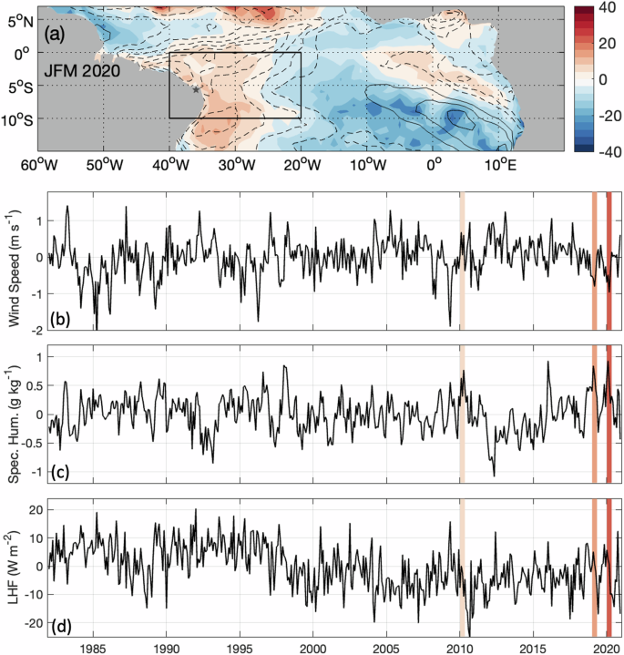
a Anomalies of wind speed (contours in m s-1) and latent heat flux (shading in W m-2) from January to March 2020. Time series of (b) wind speed (m s-1), (c) specific humidity (g kg-1) and (d) latent heat flux (W m-2) anomalies averaged for the area between 0-10°S and 20-40°W, represented by the box in panel (a). In panel (a), solid lines depict positive anomalies of wind speed and dashed lines negative anomalies; contours are every 0.2 m s-1, with zero contours omitted. The star in panel (a) represents the location of Rio do Fogo reefs (5.2°S and 35.2°W) slightly shifted to the southwest. Bars in panels b–d highlight the most severe summer/fall MHWs on record (2010, 2019, 2020) coloured by severity.
The weakening of the wind can also reduce the advection of cold waters along the equatorial region from the eastern side of the basin to the coast of South America, contributing to ocean warming in the studied area. In normal conditions, the trade winds produce westward surface ocean currents (vectors in Fig. 4a) that increase the mixed-layer depth near the coast (shading in Fig. 4a). During the summer/fall of 2020, the weakening of the trade winds reduced the advection of cold water (represented by opposing currents in Fig. 4b). This also caused a decrease in the mixed layer depth (negative anomalies in Fig. 4b). A thinner mixed layer can be warmed more efficiently leading to stronger MHWs.
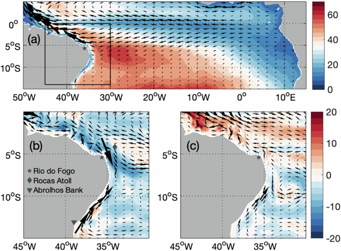
a Climatological mean of the mixed-layer depth (shading in m) and surface ocean currents (vectors in m s-1) from January to March; (b) anomalies of mixed-layer depth (shading in m) and surface ocean currents (vectors in m s-1) from January to March 2020; (c) same as (b), except for 2010.
In contrast, during the summer/fall of 2010 (the third most severe year of MHWs), there was no reduction in wind speed and no increase in the latent heat flux (Fig. 3b, d). In addition, the surface ocean currents and mixed layer depth were not reduced (Fig. 4c) and displayed the same pattern as the climatological mean in the studied area. In 2010, the MHWs were generated by a strong increase in shortwave radiation into the ocean (positive anomalies, shading in Fig. 5a and S8e-h). This, in turn, was caused by a reduction of cloud cover depicted by negative anomalies of precipitation (contours in Fig. 5a and S8a-d) and positive anomalies of ongoing longwave radiation (shading in Fig. S8a-d). The latter is a proxy for deep convective clouds in the tropics, with negative anomalies representing more cloud cover and positive anomalies less cloud cover. Again, analysing the time evolution of these quantities over the area between 0–10°S and 20–40°W (Fig. 5b-d) shows that less cloud cover and precipitation led to more shortwave radiation and ocean warming for the summer/fall of 2010, but not for the years 2019 and 2020. Similarly to 2020, sensible heat flux and longwave radiation are negligible for the summer/fall of 2010 (Fig. S7g-h). In this case, latent heat flux has a weak cooling effect (Fig. S7e) compared to the primary driver, shortwave radiation (Fig. S7f).
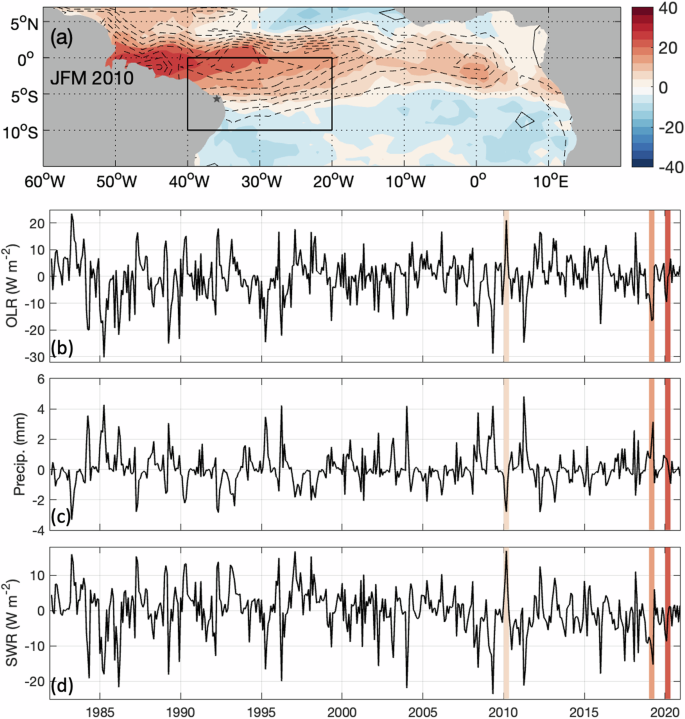
a Anomalies of precipitation (contours in mm day-1) and shortwave radiation (shading in W m-2) from January to March 2010. Time series of (b) ongoing longwave radiation (W m-2), (c) precipitation (mm day-1) and (d) shortwave radiation (W m-2) anomalies averaged for the area between 0–10°S and 20–40°W, represented by the box in panel (a). In panel (a), solid lines depict positive anomalies of precipitation and dashed lines negative anomalies; contours are every 1 mm day-1, with zero contours omitted. Bars in panels b–d highlight the most severe summer/fall MHWs on record (2010, 2019, 2020) coloured by severity.
Noteworthy to mention that even though we have an increase in the severity of the MHWs in the western tropical Atlantic, we do not see such trends in the local drivers (time series in Figs. 3 and 5). In fact, the heat flux anomalies that generated the MHWs during the summer/fall of 2019 and 2020 were much weaker than those that generated the MHWs during the summer/fall of 2010. Comparing Fig. 3a with 5a shows that in 2020, the anomalies of heat flux did not pass 15 W m-2, whereas in 2010, they reached up to 30 W m-2 in the northwest tropical Atlantic. This suggests that as the mean global ocean temperature rises due to climate change, weaker forcing (heat flux anomalies) can lead to more devastating MHWs, with implications for the survival of marine ecosystems.
Impacts of marine heatwaves on coral bleaching
The intense MHW during the summer/fall of 2020 resulted in one of the most significant bleaching events recorded along the Brazilian coast22 and at Rio do Fogo during the period of 2018–2022 (Fig. 6a–c). These reefs are critical for coral diversity in Brazil32 and have been monitored since 2018. During the summer/fall of 2020, 90% of the stony coral area was bleached (labelled S in Fig. 6d), compared to an average of 8% for the other 4 years. The situation was similar for the zoanthids; 70% of the area covered by them was bleached in 2020 against an average of 1% for the other 4 years (Fig. 6e). However, by winter 2020, both stony corals and zoanthids recovered with bleaching reducing to 10% and 8% of the area, respectively (labelled W in Fig. 6d, e). Even though 2019 was the second most extreme summer/fall in terms of MHW cumulative intensity and spatial extension in the tropical Atlantic, there was very little coral bleaching in Rio do Fogo. This is because at this location, the second most extreme summer/fall was 2010, and not 2019 (see Fig. S4 and S5). Moreover, the SST surpassed the NOAA Coral Bleaching Watch threshold of 29 °C (Fig. 2g) for approximately 4 weeks in 2019 (from mid-March to April) and 16 weeks in 2020 (from mid-January to mid-May).
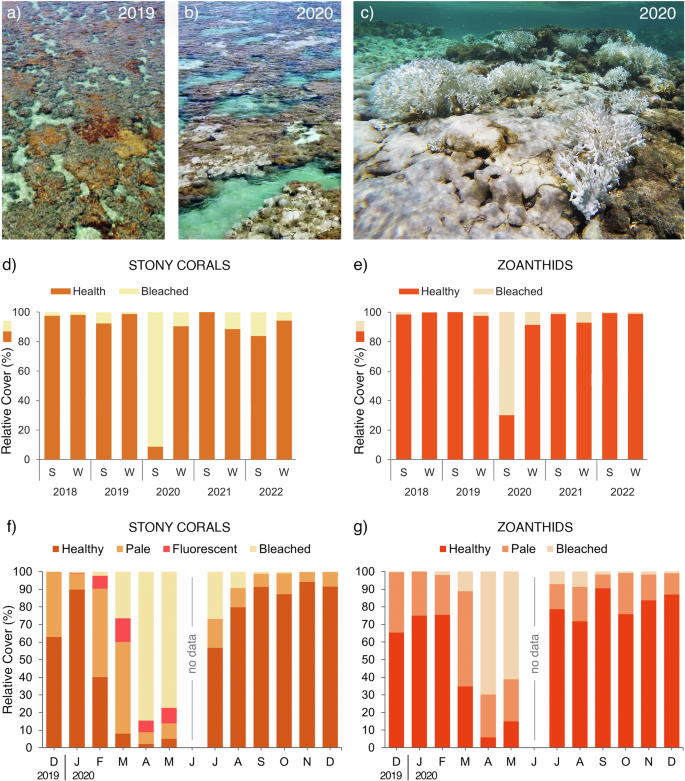
Aerial footage of Rio do Fogo reefs (a) before (April 2019) and (b) during (April 2020) the severe MHW, highlighting the changes of patches occupied by stony corals and zoanthids from a vivid brown to a stark white shade resulted from the bleaching event. c Underwater photograph illustrating the white reefscape during the bleaching event (April 2020) with most stony corals and zoanthids bleached. Summer (S) and winter (W) average percentage of the area covered at Rio do Fogo by healthy (dark shade) and bleached (light shade) for (d) stony corals and (e) zoanthids. Month average percentage of the area covered at Rio do Fogo by healthy (dark shade), pale (intermediate shade), fluorescent (pink shade; only for stony corals) and bleached (light shade) for (f) stony corals and (g) zoanthids. See methods for more details on how the coverage data are obtained.
Now, we analyse this exceptional 2020 event more closely at Rio do Fogo. During December 2019 and January 2020, stony corals and zoanthids were majorly healthy, with some regular paleness observed (Fig. 6f, g). For stony corals in February and for zoanthids in March, paleness increased, indicating a loss of photosynthetic endosymbiotic dinoflagellates. Additionally, we observed the rise of a fluorescent area for stony corals in February and March, indicating pre-bleaching stress (Fig. 6f). From April on, considerable bleaching was observed, peaking in April with 85% of stony corals and 70% of zoanthids areas bleached (Fig. 6f, g). In May, stony corals and zoanthids were still heavily bleached (77% and 61%, respectively). From May to August, the bleached area decreases consistently and becomes negligible from September on, when most stony corals and zoanthids return to healthy status (90% and 75% of the healthy area, respectively), with occasional paleness.
One could argue that analysing one site is not enough to associate coral bleaching with MHWs in this region. Even though bleaching episodes of comparable magnitude are rare in the tropical South Atlantic, earlier studies reported a similar rare event in Rocas Atoll and Abrolhos Bank in 2019, where over 80% of the stony corals bleached19,20. At both sites (see Fig. 4b for their locations), coral mortality was low, except for the hydrocoral Millepora alcicornis. Also, major coral bleaching and mortality occurred in the same period in other areas of the western tropical Atlantic and were linked to the 2019 MHWs23. For the historical period analysed here, this coincides with the second most severe summer/fall on record in terms of MHWs (Fig. 1e and Tabs. S1-S2). Another exceptional bleaching event occurred in 2010 that caused the bleaching of 80% of stony corals in Todos os Santos Bay33 (south of our domain at 18°S). Again, this exceptional event of 2010 occurred during the third most severe summer/fall in terms of MHWs (Fig. 1e and Tabs. S1-S2). Moreover, none of these previous studies was able to directly link the bleaching events to MHWs or reported such massive bleaching of stony corals concomitantly of zoanthids as the one studied here. This suggests that these severe MHWs are a precursor for massive coral bleaching events in the region. Still, zoanthids tend to be more tolerant to thermal stress and suffer less bleaching, corroborated by earlier studies for other locations in the South Atlantic and South Pacific34,35,36.
In addition, we looked at turbidity (Fig. S9), which can be another key factor for coral bleaching. Previous studies have shown that a combination of a warm environment with increased light penetration into the coral skeleton due to the loss of coral tissues, coupled with coral tissue decay, supports rapid microbial growth in the skeletal microenvironment, resulting in the wide degeneration of the coral skeletons17. This indicates that turbidity can protect the coral from bleaching during a warming event, including along the coastal regions of the tropical Atlantic37. So, MHWs combined with a reduction of turbidity can be more devastating. This is particularly important during MHWs caused by a reduction of cloud cover and precipitation, such as those in 2010. In addition to the lack of clouds (more shortwave radiation), less precipitation over land means less river discharge and less turbidity. On the other hand, the MHW events caused by latent heat flux, such as those in 2019 and 2020, are not necessarily associated with a reduction in turbidity. Indeed, turbidity at Rio do Fogo in the summer/fall of 2010 was the lowest on record, reaching −4 × 10⁻³ m-1 below average. In contrast, during the summer/fall of 2019 and 2020, turbidity was above average (Fig. S9). Therefore, if conditions similar to those of 2010 happen now, the devastation could be even worse.
Conclusions
The tropical Atlantic is the smallest of Earth’s tropical ocean basins and, as such, interacts intimately with adjacent continents, strongly influencing their weather and climates. Many studies have investigated the role of tropical Atlantic variability on extreme events such as floods and droughts in West Africa and South America, intense storms and hurricanes38,39,40. However, little is known about physically defined ocean extremes (MHWs) in the tropical Atlantic that can amplify the vulnerabilities of regional marine ecosystems – systems already stressed by overfishing and pollution – and jeopardise local economies and food sources. By causing bleaching and coral loss, severe and recurrent MHWs can potentially reduce diversity and reef complexity, having a negative impact on the benefits provided by the reefs to humans41.
Here, we show that MHW events in the tropical Atlantic have increased in frequency, intensity, duration, and spatial extent. MHWs are 5.1 times more frequent and 4.7 more intense since the records started in 1982, with the 10 most extreme summers/falls in terms of MHW cumulative intensity and spatial extension occurring in the last two decades. The long-term trend in extreme warming (MHW cumulative intensity) occurs mainly in the western tropical Atlantic, where the mean SST is already at its highest, with potential implications for marine ecosystems.
The positive trend in extreme warming is associated with a weakening of the trade winds in the region. This, in turn, reduces the ocean’s capability of cooling by decreasing latent heat flux from the ocean to the atmosphere and weakening the advection of cold waters to the area. These processes were responsible for the extreme warming during the summer/fall of 2020, which led to severe coral bleaching in Rio do Fogo. Considerable bleaching was observed, with 85% of stony corals and 70% of zoanthids areas bleached by April after a sequence of 5 MHWs of 32, 19, 11, 19 and 9 days of duration categorised from moderate to strong events. Our study also shows that soft corals (zoanthids) are more resilient than reef-building coral during MHWs.
The study also shows that another physical mechanism generates MHWs in the region. The lack of clouds in the region can lead to more shortwave radiation into the ocean and thus MHWs that, combined with less rainfall, can decrease turbidity and lead to coral bleaching. This mechanism was responsible for the MHWs in the summer/fall of 2010, with several bleaching events in the region reported in the literature. In addition, we notice that even though we have an increase in the severity of the MHWs in the western tropical Atlantic, we do not see trends in the strength of the local drivers, i.e., latent heat fluxes or shortwave radiation. This suggests that as the mean global ocean temperature rises due to climate change, weaker forcing can lead to more devastating MHWs, with implications for the survival of marine ecosystems.
It is also worth mentioning that we have only analysed the local drivers of the MHWs. The local processes described here can, in turn, be triggered by remote drivers, such as ENSO. However, we cannot say ENSO is a remote driver because 2009/10 was a strong central Pacific El Niño year, 2018/19 a weak El Niño year, and 2019/20 a neutral year. The 2018/19 and 2019/20 events have the same local drivers but different ENSO conditions. There is not a consistent relationship. Unfortunately, it is difficult to make statistically robust links between ENSO and these extreme events because they are, by definition, rare events with few realisations for 1982–2022.
In spite of the aforementioned limitations, we hope that improving our understanding of the physical drivers of MHWs and their impact on corals will be vital for better predicting these events. The latter can, in turn, guide adaptation and mitigation policies to avert the most severe impacts on marine ecosystems.
Methods
Defining marine heatwaves and data sets
To identify the MHW events, we use daily gridded SST data obtained from the National Oceanic and Atmospheric Administration Optimum Interpolation Sea Surface Temperature (OISST) V2.0 with a horizontal resolution of 1/4° for the period 1982–202242. Following the standardised MHW definition43, an MHW event occurs when SSTs exceed a seasonally varying 90th percentile for a minimum of five consecutive days. An event is considered continuous even if gaps of two days or less between events occur. In accordance with recent literature44 and the purpose of this study, we use a fixed baseline (1982–2020 climatology). Here, we also calculate the severity of each MHW event using a simple categorisation scheme31. Our analysis focuses on three MHW metrics: frequency (total number of days of MHWs per year), spatial extension (percentage of the total area with MHW) and cumulative intensity (integral of intensity over the span of every event per year). The latter has a higher ecological significance and considers both the mean intensity and duration of every event. Moreover, this metric is more advantageous than the Degree Heating Week (DHW) approach, which represents the duration of thermal anomalies experienced by corals, accumulated across three months45. As such, the DHW cannot detect extreme acute events that also cause substantial coral bleaching17,46,47. The MHW approach also has many advantages over the commonly used methods of fixed anomaly above the local mean SST or fixed temperature threshold because it accounts for both local SST climatology and its variance, which can control local communities and their thermal tolerance. Nonetheless, we have computed the mean maximum temperature for the summer, referred to as the summer maximum used in the DHW methodology as the thermal tolerance limit. The NOAA Coral Bleaching Watch determines that, for any given area, water temperatures of 1 °C above the expected summertime maximum temperature are stressful to corals, and the area is considered a coral bleaching hot spot. For our region, the summer maximum is 28 °C and occurs in March and April. The highest value ever recorded from the OISST dataset is 30.3 °C. So, we consider 29.0 °C, 29.5 °C and 30.0 °C thresholds to represent the extremes of absolute SST beyond the thermal tolerance limit defined as the summer maximum (28.0 °C) and, as such, when our location becomes a potential coral bleaching hot spot in agreement with the literature24,48.
Defining the drivers and statistical analysis
Long-term trends of SST and MHW cumulative intensity are calculated using a linear least-squares fit from 1982 to 2022, and the nonparametric test of Mann-Kendall is used to assess their significance at the 95% confidence level. To rank the 10 most extreme summer/fall MHW events for the tropical Atlantic (Tab. S1), we first normalise the cumulative intensities for each year by the most extreme cumulative intensity on record (for the event of 2020) and multiply by 100 to get similar units to those of spatial coverage (in %). Then, for each year, we multiplied the normalised cumulative intensity by their respective spatial coverage. We then use this index to rank the MHW events. The only event before 2000 that ranked in the top 10 was 1998, so for simplicity, we state that the 10 most extreme summers/falls in terms of MHW cumulative intensity and spatial extension occurred in the last two decades. To determine the increase in frequency and intensity of the MHWs, we first compute their respective mean decadal values (1982–1991, 1992–2001, 2002–2011, 2012–2021). Then, we compare the mean frequency and intensity for the last decade with those for the first decade, dividing the former by the latter. This method is used instead of analysing the linear trend to avoid potential bias in the trends due to the beginning and end values.
To investigate the drivers of the MHWs in the tropical Atlantic, we compute the composites of various atmospheric variables obtained from the European Centre for Medium-Range Weather Forecasts (ECMWF) ERA-5 reanalysis for the same period49. Daily values are obtained by averaging the hourly data of surface heat fluxes, surface specific humidity, zonal and meridional components of the wind at the surface and 850 hPa. We also use the gridded daily rainfall data provided by the Global Precipitation Climatology Project (GPCP) with a horizontal resolution of 2.5° for the period 1997–202250 and the interpolated outgoing longwave radiation (OLR) daily data51 as a proxy for tropical convection, with the same spatial resolution for the period of 1982–2022. The diffuse attenuation coefficient at 490 nm from the NOAA-MODIS satellite for the period 2003–202252 is used as a proxy for turbidity of the water column. For clarity, we plot monthly averages in Figs. 3, 5, S9.
Defining coral bleaching events and data sets
To assess the ecological impacts of the MHWs during the summer/fall of 2020 on the tropical shallow reefs off the northeast coast of Brazil, we analyse the health status of stony corals (reef builders with the hard skeleton; Cnidaria: Anthozoa: Scleractinia) and zoanthids (soft-bodied colonial cnidarians with no hard skeleton; Cnidaria: Anthozoa: Zoantharia). We survey 6 fixed 20 m transects (1-2 m deep) in the shallow patchy reefs of Rio do Fogo (5.2°S, 35.2°W), and sample them monthly from December 2019 to December 2020, comprising surveys before, during, and after the MHW. We collect coral bleaching data during the austral summer and fall because the waters are the warmest in this period (Fig. 2g). During the surveys, we take 10 photographs (0.5 × 0.5 m) evenly distributed along each transect. For the photographs with stony corals and/or zoanthids, the health status data is obtained by quantifying how much of the area covered by them is 1) healthy (dark vivid shade; high density of dinoflagellates), 2) pale (light shade; low density of dinoflagellates), 3) fluorescent (pink/purple shade; indicative of pre-bleaching stress in stony corals), or 4) bleached (stark white shade; negligible density of dinoflagellates). Coverage data are then obtained by averaging the data of each health status category from the photographs for any given month in which stony corals and/or zoanthids were present.
In addition, to assess how severe the 2020 bleaching event is compared to other recent years, we used data from surveys of benthic assemblages conducted in the study area from 2018 to 2022. Each year, stony coral/zoanthid cover and health status data are collected during late summer (March or April), when bleaching typically peaks, and during winter (July or August), when corals/zoanthids return to a healthier status. These data are monthly averaged from photographs taken along random transects. The number of photographs varies from 90 to 200, depending on the sampling month. We quantify the relative percentage of the area covered by stony corals/zoanthids that is healthy (any shade of colour; the presence of dinoflagellates) or bleached (stark white shade; negligible density of dinoflagellates). To determine mortality through time (loss of coral cover), we measured total stony coral/zoanthid cover (percentage area covered in the quadrat) for each time step.
Reporting summary
Further information on research design is available in the Nature Portfolio Reporting Summary linked to this article.


Responses