Climate simulations and ice core data highlight the Holocene conundrum over tropical mountains

Introduction
The Holocene (11 ~ 0 ka before the present) is the latest interglacial period characterized by a relatively stable and warm climate compared to that of the preceding deglaciation (20 ~ 11 ka). Despite the relatively smaller magnitude of climate change in the Holocene compared to the deglaciation, the understanding of Holocene climate evolution still poses significant challenges. A key issue arises from the contrasting temperature trends in the global mean surface temperature (GMST) between paleoclimate proxies and climate models. Temperature reconstructions derived from various sources such as alkenes in ocean sediments, foraminifera Mg/Ca ratio, lake sediments, pollen, ice cores, and speleothems consistently indicate a thermal maximum in the early-to-mid Holocene, when the estimated GMST was approximately 1 °C higher than at present, followed by a gradual cooling from the mid to late Holocene1,2. In contrast, the state-of-the-art climate model simulations suggest continuous GMST warming throughout the Holocene with no distinct thermal maximum3,4. Model ensembles from the Paleoclimate Model Intercomparison Project (PMIP) estimate a cooling of 0.3 ~ 0.5 °C in the mid-Holocene compared to the present3,4. This discrepancy between climate models and proxies, which is referred to as the Holocene temperature conundrum3, indicates potential uncertainties in both the proxy data and climate models. A portion of marine sediment and pollen proxies imprint signals to specific seasons associated with organism growth, and thus do not represent the annual mean temperature5,6,7. After removing the seasonal signal from planktic foraminifera records in the tropics using a semi-statistical transformation method, the reconstructed annual mean sea surface temperature (SST) in the tropics, and likely over the globe, exhibits a warming trend throughout the Holocene as suggested by climate models6, although this transformation method remains in debate8. Climate model uncertainties may stem from model resolution, sub-grid parameterization, inaccurate or missed feedback processes such as Arctic sea ice9, vegetation10, anthropogenic land use11, dust12, and volcanic sulfur emissions2,13. Data assimilation by combining proxy records and climate models produces either a weak warming trend14 or a slight thermal maximum in the mid-Holocene15. The discrepancy between models and proxies remains unresolved both globally and regionally, particularly over land areas characterized by spatial heterogeneity. Resolving this discrepancy is critical for increasing the accuracy of future climate model projections.
In this study, we conducted the transient simulation of the Holocene (11 ~ 0 ka) climate using an isotope-enabled earth system model (iTRACE) to rigorously constrain the climate model with paleoclimate tracers and better understand Holocene climate variability. The simulated δ18O in precipitation (δ18Op) and associated climate variables from iTRACE are then used to drive a forward ice core proxy system model (PSM) PRYSM developed by Dee et al.16, which simulates δ18O in ice core (δ18Oice), thereby enabling a direct model-data comparison of δ18Oice records. Our direct comparison between the modeled and measured δ18Oice provides a more robust model evaluation with two key advantages: (1) it ensures a fair comparison by weighting iTRACE δ18Op with monthly precipitation before driving PRYSM, which mitigates the influence of proxy biases toward specific seasons, and (2) it avoids the need to convert proxy records to temperature, thereby introducing fewer errors. We will focus on δ18Oice records only from Greenland, Antarctica, and tropical mountains, as glaciers in these regions are sensitive to temperature changes17,18, and their moisture sources and climate signals are generally clearer and more regionally representative compared to those from mid-latitudes19. The representation of δ18Oice for the in-situ condensation temperature, the so-called temperature effect, has long been confirmed in Greenland and Antarctica20,21 over different time scales, as well as over tropical mountains during the last deglaciation (20 ~ 11 ka)17,18,22,23. This close δ18O-temperature relationship is fundamentally controlled by the Rayleigh distillation process20. However, the local temperature signal preserved in δ18Oice is also modified by changes in moisture source, transportation pathway, precipitation seasonality24, ice sheet elevation25, ice flow, and post-deposition processes, including wind-driven redistribution, diffusion, and vapor-snow exchange26. These may lead to differences in δ18Oice trends and may distort the Holocene climate signal over Greenland and Antarctica (Supplementary Notes 1). Nevertheless, consistent δ18Oice (after removing the effect of ice elevation changes or ice sheet thinning due to ice melting and sea level rise) and borehole temperature signals may still exist over Greenland, with early (8 ~ 9 ka) and the mid-Holocene (5 ~ 6 ka) temperatures that are ~3 °C and 2 ~ 2.5 °C warmer than those in the pre-industrial (PI), respectively25,27,28. Carefully selected Antarctic δ18Oice records show a heterogeneous east-west temperature response in Antarctica (Supplementary Notes 1). A preliminary temperature estimate for Antarctica, utilizing a weighted average from six δ18Oice records that are biased toward the plateau ice cores, suggests a 1 ~ 2 °C warming during the early Holocene optimum, without a noticeable difference in the mid-Holocene compared to the PI29.
Tropical mountain ice cores drilled near the ice divide from relatively flat ice caps in the Andes may provide valuable tropical climate signals without being strongly influenced by ice flow30 and moisture source changes (as the moisture here comes mainly from the upstream Amazon Basin and the equatorial Pacific18,31,32,33,34,35). More interestingly, the evolution of proxy δ18Oice records from Kilimanjaro and Huascarán largely resembles those from sites peripheral to Greenland (e.g., Agassiz and Renland), even quantitatively. The δ18Oice values from Renland and Huascarán exhibit a decrease of 1.5‰ and 2.1‰, respectively (Fig. 1j and n; Table 1), possibly indicating a dynamically uniform temperature response in the tropical upper troposphere and the polar lower troposphere. If tropical mountain δ18Oice represents the in-situ temperature change, as is the case for the deglaciation period18,23, the isotopic depletion in δ18Oice may suggest a cooling trend from the early to the late Holocene. This seems to be supported by the ice cap advance (and cooling) from the mid (~7ka) to late Holocene inferred from buried rooted plants collected from Quelccaya (14oS) ice margin36. However, the carbonate clumped isotopes (Δ47) from Lake Junin, Pumacocha, and Mehcocha (~11 °S) suggest that carbonate formation temperatures were relatively constant (as opposed to a cooling trend) throughout the Holocene compared to the present, though these estimates come with relatively large uncertainties (over (pm)2 °C)37. When combining temperature estimates from the Amazon basin38 and the Andean foothills39, it appears that relatively stable Holocene temperatures might be a coherent feature across the tropical South America region. The apparent divergent proxy temperature estimates highlight an ongoing debate regarding the interpretations of tropical mountain δ18Oice during the Holocene: whether it reflects a temperature change17,18,23 or reflects hydroclimate changes, including precipitation, upstream moisture condition, or monsoon intensity. The latter are inferred mostly from lacustrine sediments or speleothem records37,40,41,42,43,44,45. Further investigation is required to clarify the interpretations of stable water isotopes retrieved from ice core proxies, with the aid of climate model simulations.

a Annual mean orbital-induced solar insolation forcing (W/m2) at 65°N (red), 15°S (black), and 75°S (blue); (b) Orbital-induced insolation forcing (W/m2) at 65°N (solid lines), 15°S (dash dotted lines), and 75°S (dashed lines) in DJF (blue; left axis) and JJA (red; right axis); (c) Global mean atmospheric CO2 concentration (ppm); d Global ice volume change (105 km3) relative to the Last Glacial Maximum; e231Pa/230Th reconstructed from sediment core GGC5 as a proxy for AMOC intensity (black) and model AMOC intensity (blue); f Geographical location of ice cores used in this study; (g–q) Time series of proxy δ18Oice averaged over 100-year bins (‰; black), model annual δ18Oice (‰; gray), and model δ18Oice averaged over 100-year bins (‰; blue) from: (g) Agassiz94; (h) Camp Century95; (i) NGRIP96, (j) Renland94, (k) Dye 396, (l) Penny97, (m) Kilimanjaro98, (n) Huascarán23, (o) Sajama22, (p) Dome C99, and (q) WAIS David54. The yellow and blue filled shadings denote the mid-Holocene and PI, respectively. Solar insolation values in (a) and (b) are the differences respective to 11 ka.
For the background information, the features of δ18Oice during the Holocene, based on a compilation of ice core records from Greenland, Antarctica, and tropical mountains, are thoroughly discussed in Supplementary Notes 1. Then, we present the direct model-proxy data comparison of δ18Oice at different ice core sites and then discuss temperature change throughout the Holocene. We show that when compared to most Greenland proxy δ18Oice records, the model simulates a weaker early Holocene maximum and a weaker decreasing trend in δ18Op and δ18Oice in the mid-to-late Holocene. Surprisingly, the model shows an opposite trend when compared to the δ18Oice records from equatorial mountains throughout the Holocene. This discrepancy highlights the Holocene δ18O conundrum over the tropical mountains. We propose several hypotheses regarding the forcing mechanisms of the Holocene δ18Oice changes and discuss possible model deficiencies that may explain the model-data inconsistency.
Results and Discussion
Ice core δ18O and temperature evolution in the iTRACE model
As the iTRACE model does not account for post-depositional processes in ice cores, we further utilize its output to drive a forward ice core PSM (see Methods). This enables a direct comparison between the model-derived δ18Oice and the proxy-derived δ18Oice at each ice core site. Notably, the model δ18Oice reflects the signal for precipitation-only events. To ensure a consistent comparison, the model surface temperature is also weighted by monthly precipitation. Our comparison and analysis will focus mainly on the variability (considering anomalies rather than absolute values) in δ18Oice over millennial and longer time scales. Therefore, we perform multi-channel singular spectrum analysis (MSSA) on time series from all ice core sites and examine the leading reconstruction component of the MSSA, which captures the mode of the long-term trend through the Holocene (see Methods).
Greenland
Across all Greenland ice core sites, the model δ18Oice shows a synchronous evolution with δ18Oice increases from the early-to-mid Holocene (10 to 7 ka), followed by stable or slight decrease from the mid-to-late Holocene (Fig. 1g-l: blue lines), with a weak δ18Oice peak in the mid-Holocene (7 ~ 6 ka) compared to the proxies, except at Agassiz and Penny. The δ18Oice evolution is a response to boreal summer and annual insolation change (Fig. 1a and b), which slightly increase in the early Holocene and then decrease in the mid-to-late Holocene due to the changing precession from boreal summer to winter. In comparison with proxies, model δ18Oice shows three main discrepancies. First, the model δ18Oice evolves almost synchronously across all Greenland sites, while proxies show rather asynchronous responses based on the geographical features of the location (Supplementary Notes 1). Second, the magnitude of the Holocene peak in the early-to-mid Holocene (i.e., δ18Oice response between the peak stage and PI) is weaker by a factor of 2 ~ 4 at most sites (Fig. 1g-l; Table 1), except on Agassiz and Penny where the response of model δ18Oice magnitude is comparable to that of proxies. During the mid-to-late Holocene, the correlation coefficient of δ18Oice between the model and proxies ranges from 0.2 to 0.7 (Table 1), indicating a moderate model-data agreement. Third, the model δ18Oice reaches its maximum approximately 2 ka later than that of proxies at most sites (Fig. 1g–l; Table 1). The relatively weak δ18Oice peak and synchronous evolution in the model, compared to proxies, may be explained by the absence of certain local feedbacks (e.g., moisture conditions and vertical lapse rate46) and smoother topography in the Greenland region due to coarse model resolution, which may result in a more uniform climate response. The relatively late model δ18Oice peak in the early-to-mid Holocene can be partially attributed to the overestimation of the response of Atlantic Meridional Overturning Circulation (AMOC) to meltwater forcing in the model47, which produces weaker and slower warming during the early Holocene in high latitudes. Additionally, the model δ18Oice exhibits two cycles of centennial variability (observed in both δ18Oice and temperature) after the 8.2 ka event. These variations align with large-amplitude changes in model AMOC during 8.2 ~ 7.5 ka that are not evident in the 231Pa/230Th-derived AMOC intensity (Fig. 1e). Consequently, these centennial-scale variations are likely unrealistic and may result from an inadequate meltwater scheme in the simulation. However, this limitation does not significantly impact our discussion of the long-term trend.
The leading mode of the MSSA suggests that the model arithmetic annual mean surface temperature (({T}_{s}^{{uw}}): unbiased 12-month average, as opposed to an annual mean weighted by precipitation amount, which we introduce later) overall follows the model δ18Oice with a warming trend during the early-to-mid Holocene and a stable or weak cooling trend during the late Holocene at most Greenland sites (Fig. 2a1-a6). However, the evolution of ({T}_{s}^{{uw}}) is slightly divergent from that of δ18Oice (Fig. 2a1-a6: blue and solid orange lines) since the model annual ({T}_{s}^{{uw}}) mainly follows the boreal winter temperature. We note that model δ18Oice is a footprint of temperature associated with precipitation events, and therefore, the seasonal cycle of precipitation should be considered for a fair comparison of Holocene temperature change. Model annual surface temperature weighted by precipitation (({T}_{s}^{{p}_{w}})) exhibits an evolution closer to δ18Oice compared to that of ({T}_{s}^{{uw}}), consistent with the isotopic temperature effect. This is also clear in a larger temporal slope of model δ18Op against ({T}_{s}^{{p}_{w}}) (({{delta }^{18}O}_{p}/{T}_{s}^{{pw}})) compared to ({{delta }^{18}O}_{p}/{T}_{s}^{{uw}}) at all Greenland sites in the Holocene (Fig. S1e-f. Supplementary Notes 2). Our results are consistent with Werner et al.48, highlighting the importance of the precipitation seasonality in explaining the discrepancy between borehole (unbiased) and isotope-inferred (biased) temperature. Existing proxy δ18Oice and borehole temperature reconstructions suggest an early Holocene warming of 2 ~ 3 °C over the Greenland ice sheet and ~4 °C over the Agassiz ice cap25,27,28,49,50. For comparison, model ({T}_{s}^{{uw}}) generally contrasts with the temperature reconstructions. In contrast, model ({T}_{s}^{{p}_{w}}) exhibits early Holocene warming at all ice core sites, with a Holocene Thermal Maximum (HTM) ranging from 0.12 to 3.52 °C and an average of 1.0 °C, which is overall weaker than observations by a factor of 2. The underestimation of the model temperature response over Greenland could be attributed to the model’s weak sensitivity to orbital-induced insolation forcing3.
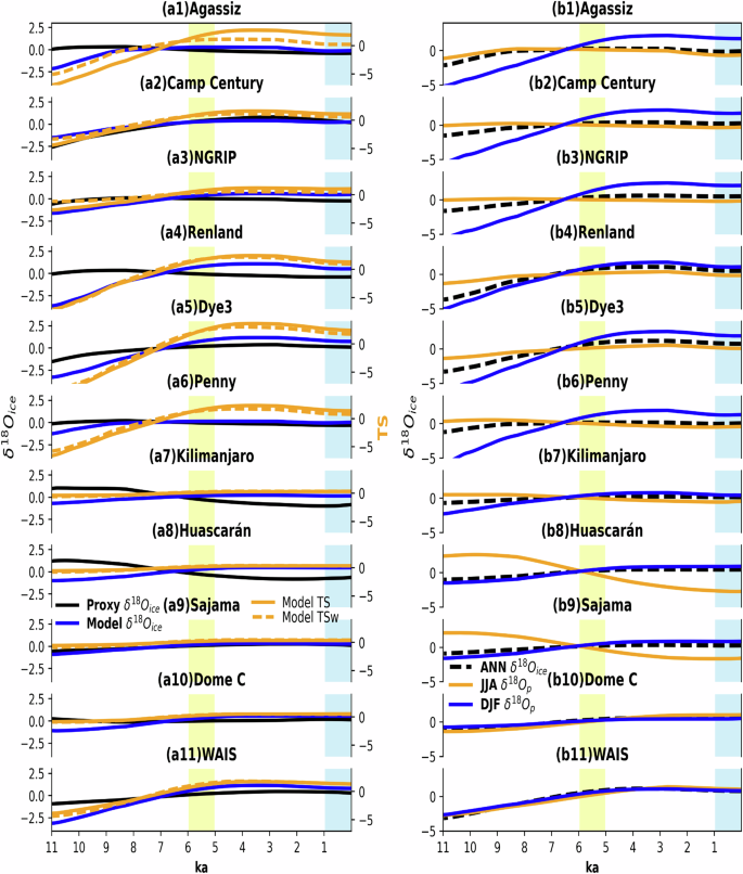
The leading reconstruction component (long-term trend) of the MSSA (see Methods) for the time series of annual (a1-a11) proxy δ18Oice (‰; black: left axis), model δ18Oice (‰; blue: left axis), model temperature (°C; dashed orange lines are for arithmetic annual mean ({T}_{s}^{{uw}}); solid orange lines are for annual mean weighted by monthly precipitation ({T}_{s}^{{pw}}): right axis). b1-b11 show the leading reconstruction component of the MSSA for model δ18Op during JJA (orange) and DJF (blue). Model annual model δ18Oice is included for reference (dashed black line, identical to the blue line in a1-a11). The eigenvalues, or variance contributions, of the MSSA leading mode are 50% for proxy δ18Oice, 66% for model annual δ18Oice, 71% for model JJA δ18Oice, and 71% model DJF δ18Oice. The geographic location of each ice cores is shown in Fig. 1f.
Antarctica
The model partially reproduces the evolution of Antarctic δ18Oice throughout the Holocene. The model δ18Oice for Dome C in the East Antarctic shows a gradual isotopic enrichment in the early-to-mid Holocene and then a stabilization in the late Holocene (Fig. 1p: blue line; Table 1). In contrast, proxy δ18Oice reaches its maxima in the early Holocene (11 ~ 9 ka), followed by a decrease during 9 ~ 7 ka (Fig. 1p: black line). The early Holocene maxima in the proxy is partially attributed to changes in δ18O in ocean surface waters (δ18Osw) due to decreasing ice sheet volume during the final deglaciation and the gradually intensified AMOC (Fig. 1e: black line) removed heat from the high southern latitudes51. The model δ18Oice does not produce the early Holocene maxima at Dome C, probably due to inaccurate boundary conditions and a biased model response to ice volume and meltwater forcing. For the WAIS Divide in West Antarctica, the model reproduces an increase in δ18Oice as suggested by the proxy in the early-to-mid Holocene (Fig. 1q) but shows a mismatch in the late Holocene when model δ18Oice value continues to increase while δ18Oice first stabilizes and then decreases. This may be explained by model bias in response to local insolation change, a point that will be discussed later in this section.
Unlike in Greenland, where the seasonality of precipitation is important in driving annual δ18Oice and temperature evolution, the influence of precipitation seasonality in Antarctica is negligible48,52. This is seen in the close resemblance of model δ18Oice evolutions among different seasons (Fig. 2 b10-b11) and the similarity in model annual ({T}_{s}^{{uw}}) and ({T}_{s}^{{p}_{w}}) evolutions (Fig. 2 a10-a11: comparing dashed and solid orange lines). Thus, only ({T}_{s}^{{uw}}) is used when referring to surface temperature in Antarctica. The model ({T}_{s}^{{uw}}) follows δ18Oice throughout the Holocene, with a gradual warming in the early-to-mid Holocene and a warming hiatus in the late Holocene. A compilation of proxy δ18Oice from the East Antarctica plateau and coast suggests an HTM (11 ~ 9 ka) of ~1 °C compared to the PI climate (Supplementary Notes 2), while no discernible change is evident in the mid-Holocene29 (red line in Fig. S2b). In contrast, our model shows a continuous warming of 1.7 °C from 11 to 3 ka and a missing HTM at Dome C (Fig. 2a10: orange lines; Fig. S2b), driven by increased DJF insolation and CO2 concentration. For West Antarctica, independent borehole temperature records from the WAIS Divide53 (red line in Fig. S2c) suggest a gradual warming from 8 to 3.5 ka, reaching a steady thermal maximum of ~1.5 °C (compared to the PI) and ~1 °C cooling after 1.5 ka. The high-resolution seasonal temperature derived from the WAIS Divide calibrated isotope records54 indicates a dominant role of summer on the annual mean temperature during the mid-to-late Holocene (comparing orange and red lines in Fig. S2c), likely driven by local maximum insolation in December (green line in Fig. S2a)54. For comparison, our model also exhibits a weak thermal maximum (offset 1 ka to 9 ~ 8 ka) followed by a comparable warming (1 ~ 1.5 °C) from 8 to 3.5 ka and then a warming hiatus in the late Holocene (Fig. 2a11: orange lines; Fig. S2c), driven by increased mean DJF insolation during the mid-to-late Holocene.
Tropical Mountains
Direct model-data comparisons of δ18Oice over tropical high mountains are challenging because the coarse model resolution cannot resolve the small-scale isolated high mountain peaks of these ice core sites. However, since the variability of δ18Op is highly correlated with and condensed from the environmental vapor δ18O (δ18Ov)55, we treat the model δ18Ov at the height of the ice core site as an approximation of the model δ18Op, following our recent work18. To enable a direct comparison of δ18Oice between proxy and model at the same altitude, we first establish a linear relationship between the model near-surface δ18Ov and δ18Op, as these two are typically in equilibrium. Assuming this linear relationship remains constant with height, we can calculate a pseudo-δ18Op at the ice core altitude based on the model δ18Ov. This pseudo-δ18Op is then used to force the ice core PSM model, yielding the final tropical mountain δ18Oice for direct comparison. Note that the model annual mean δ18Ov is also weighted by monthly precipitation (({delta }^{18}{O}_{v}^{{pw}})) at each ice core site to mimic the δ18O in precipitation (δ18Op) and, in turn, the δ18Oice. This weighted average approach also accounts for the fact that tropical mountain δ18Oice signal may be highly biased toward wet seasons, as much of the accumulation occurs during the wet season and the reduction of snow height by sublimation and wind scour tends to modify and remove the dry season signals31,56,57,58.
In contrast to the polar regions, where the model generally reproduces the δ18Oice evolution observed in proxies, albeit with a much weaker amplitude (Fig. 1; Table 1), the evolutions of model δ18Oice throughout the Holocene are opposite to that observed in proxies from Kilimanjaro, Huascarán (Fig. 1m and n; Fig. 3c, d), and Illimani59 (gray line in Fig. 3c, but for δDice). Specifically, the model δ18Oice shows an isotopic enrichment of 0.8 ~ 1.8‰ from the early to the late Holocene, while the proxy δ18Oice exhibits an isotopic depletion of 1.5‰ (Table 1). This is surprising, given that the model is in good agreement with the proxy δ18Oice at Huascarán during the last deglaciation and is proven to be an indicator of air temperature18. Further analysis indicates that the increase in the model annual δ18Oice is largely driven by its increasing trend during the wet season or DJF (Fig. 2b8), although the dry season (JJA) exhibits a decreasing trend similar to that observed in proxies. Unlike Kilimanjaro and Huascarán, the model δ18Oice evolution aligns quantitatively with that of Sajama, a near-subtropical ice core, (Fig. 1o), exhibiting a long-term trend similar to δ18Oice at the WAIS Divide.
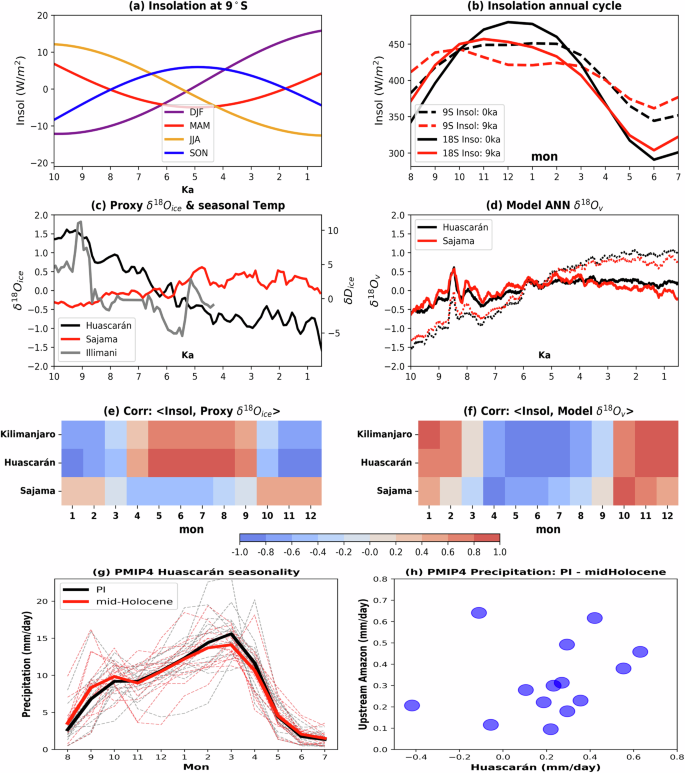
a Time series of seasonal mean solar insolation at 9°S (W m-2). b Seasonal cycle of solar insolation at 9°S (Huascarán latitude) for 0 ka (dashed black) and 9 ka (dashed red), and at 20°S (Sajama latitude) for 0 ka (solid black) and 9 ka (solid red). c Time series of proxy δ18Oice records (‰) from Huascarán (black: left axis), Sajama (red: left axis), and δDice records from Illimani59 (gray: right axis). d Time series of model annual mean δ18Ov at the ice core altitude of Huascarán (black) and Sajama (red). Solid lines are for the arithmetic annual mean (({delta }^{18}{O}_{v}^{{uw}})) and dashed lines are the annual mean weighted by monthly precipitation (({delta }^{18}{O}_{v}^{{pw}})). e Correlation coefficient between δ18Oice and 9°S solar insolation for each month throughout the Holocene at each ice core site. f Correlation coefficient between model arithmetic annual mean δ18Ov and 9°S solar insolation for each month throughout the Holocene. Note that time series in (a), (c), and (d) are shown as anomalies from the climatological mean. g Seasonality of precipitation at Huascarán derived from PMIP4-CMIP6 simulations (including the iTRACE) for the mid-Holocene (red) and PI (black). Solid lines are the results of multi-model ensembles, and dashed lines are for each model. h Annual precipitation differences (PI minus mid-Holocene) over Huascarán and upstream Amazon region derived from PMIP4-CMIP6 simulations (including the iTRACE). Each dot represents a single model.
The model annual mean temperature (we only discuss ({T}_{s}^{{uw}}) here given the similarity between ({T}_{s}^{{uw}}) and ({T}_{s}^{{p}_{w}}) in the tropics) follows the model annual δ18Oice at the same altitude, with a gradual warming of ~1.5 °C throughout the Holocene at the three tropical mountain ice core sites (Fig. 2a7-a9), which is comparable to the magnitude of the general upper-troposphere warming in the tropics (Fig. S5a and c). Despite the absence of independent temperature records reconstructed from the ice cores, the warming trend suggested by the iTRACE model does not appear to be supported by limited temperature estimates from lacustrine sediments, derived from either carbonate clumped isotopes37 or Branched glycerol dialkyl glycerol tetraethers (brGDGTs)60. These estimates suggest a likely stable temperature throughout the Holocene, albeit with about (pm)2 °C uncertainties. Furthermore, even if δ18Oice reflects the in-situ temperature change during the Holocene (as is the case during the last deglaciation), one would estimate a 0.8 ~ 1.8 °C cooling at Kilimanjaro and Huascarán from the early to late Holocene, contrasting with the warming trend suggested by the model. In contrast, an estimated 1.0 °C warming at Sajama would be comparable to the model results (Supplementary Notes 2). Our preliminary analysis reveals the challenges of rigorously estimating Holocene temperature changes and reconciling the differences among various proxies and climate models over the tropical mountains.
The Holocene Conundrum in tropical mountain ice core δ18O
Although the model tends to underestimate the δ18Oice trend in polar regions, the forcing mechanisms there are relatively straightforward: polar δ18Oice responds primarily to Holocene insolation forcing through a robust isotopic temperature effect (see above discussions). However, the forcing mechanisms of the isotopic trend observed in tropical mountain δ18Oice remain unclear and, therefore, pose the Holocene Conundrum in tropical mountain δ18Oice change. Taking the Huascarán ice core as an example (and similarly for the Illimani ice core), the present-day observations suggest a strong seasonality of precipitation at the Huascarán site (Fig. S3b6; Fig. S4b2), with a single peak from December to March and the corresponding δ18Oice and δ18Op minimum (but offset a month toward April as shown in Fig. S4c2). If we assume the Holocene δ18Oice is an indicator of annual temperature change dominated by local processes, one should expect a warming trend and an increase in proxy δ18Oice throughout the Holocene in response to increasing insolation in the wet season (DJF) (Fig. 3a) when perihelion is shifting toward austral summer. This expected warming and δ18Oice increase are produced in the iTRACE model but are opposite to the δ18Oice decrease observed in ice core records (Fig. 1n; Fig. 3c, d), raising the puzzle here. A similar case is evident in the Kilimanjaro ice core, where the seasonal cycle of precipitation shows two peaks as the Inter-Tropical Convergence Zone (ITCZ) passes over 3 °S twice a year (Fig. S3b5). Under the same assumptions, we should expect weak warming and an associated δ18Oice increase in response to a weak increase in wet season insolation (Fig. 3a), as shown in the iTRACE model instead of the long-term decreasing trend observed in Kilimanjaro proxy δ18Oice (Fig. 1m). Therefore, we raise a key question here: What drives the decrease in δ18Oice in the near-equator region, as observed in the Huascarán (9 °S), Kilimanjaro (3 °S), and Illimani (16.6 °S) ice cores? Proposing several hypotheses to these questions will be helpful in explaining the model-proxy discrepancy on tropical mountain δ18Oice evolution throughout the Holocene.
Despite a significant negative correlation (r < −0.7; p < 0.01) between solar insolation flux and proxy δ18Oice values during the wet season (DJF) (Fig. 3e), a significant positive correlation (r > 0.7; p < 0.01) between the two is found from May to September (Fig. 3e) for Kilimanjaro and Huascarán (and also Illimani). This suggests one explanation (Hypothesis I): that the seasonality of precipitation may shift gradually from DJF to JJA or SON throughout the Holocene, assuming proxy δ18Oice serves as a signal of the local temperature during the wet season. In other words, decreasing SON (or JJA) insolation during the mid-to-late Holocene may drive a decreasing δ18Oice associated with a cooling trend. This hypothesis seems to be supported by a shift of the insolation maxima from DJF toward SON at 9 °S in the early Holocene compared to the PI (Fig. 3b: comparing black and red dashed lines). Correspondingly, we examine the precipitation seasonality changes over the tropical Andes from iTRACE and PMIP4-CMIP6 models. However, most models indicate minimal changes in the seasonality of precipitation from the mid-Holocene to PI, consistently showing a wet season during DJF (Fig. 3g). Similarly, the seasonality change of the model δ18Ov over Huascarán is not evident (Fig. S3b6 and c6). This suggests that the temperature signal during the wet season may not be sufficient to explain the Holocene δ18Oice change observed in proxies. In contrast, the possible mechanism behind the δ18Oice changes in the Sajama ice core appears to be more straightforward. The insolation seasonality at 20 °S changes less over time (Fig. 3b: comparing black and red solid lines) and the Sajama δ18Oice may be constantly biased toward DJF (wet season) with an increasing trend due to possible warming in response to increasing insolation (Fig. 3e).
It is crucial to emphasize that the aforementioned hypothesis of seasonality changes (Hypothesis I) refers specifically to the δ18Oice signal associated with wet season or precipitation events. We also note the importance of the vapor-snow exchange process (mostly through snow sublimation) in post-deposition fractionation (increasing δ18Oice values) and thus altering the annual mean δ18O signal, especially in precipitation cessation or intermission periods26,61,62. This suggests a second explanation of forcing mechanisms (Hypothesis II) that tropical mountain δ18Oice may preserve temperature signals not only for the wet season (and precipitation events) but also for the dry season (and precipitation cessation) if the vapor-snow exchange occurs when snow is deposited and metamorphosed into ice. Although this hypothesis cannot be directly corroborated due to the absence of high temporal resolution observations in both δ18Oice and near-surface δ18Ov, we propose an alternative way to test Hypothesis II, that is, by comparing the proxy δ18Oice records with model δ18Ov in arithmetic annual mean (({delta }^{18}{O}_{v}^{{uw}})). This simple approach includes model δ18Ov signals from both precipitation events and precipitation intermissions. It’s interesting to see that the magnitudes of ({delta }^{18}{O}_{v}^{{uw}}) increase are much weaker than that of ({delta }^{18}{O}_{v}^{{pw}}) throughout the Holocene (and even a weak depletion in the late Holocene is observed: Fig. 3d) because ({delta }^{18}{O}_{v}^{{pw}}) tends to be biased toward the wet season (DJF) when solar insolation increases. The closer similarity between ({delta }^{18}{O}_{v}^{{uw}}) and δ18Oice throughout the Holocene suggests that climate signals during precipitation intermissions and dry season (when dry season cooling throughout the Holocene is driven by decreasing insolation) are also important in determining the annual δ18Ov and may influence the final δ18Oice values. However, it is important to note that strong sublimation or wind scour may remove the snow surface layer containing a dry season signal, as observed on glaciers from Cerro Tapado56, Sajama63, and Quelccaya58. As a result, δ18Oice values may be constantly biased toward the wet season. Although detailed observations from field campaigns and snow pit measurements for the Huascarán ice core are not available, instrumental observation from the nearest GNIP (Global Network of Isotopes in Precipitation) site Marcapomacocha (11.4 °S; 4400 m) indicates that over 90% of the annual precipitation falls between October and the following April. Consequently, minimal precipitation during the dry season may lead to significant sublimation and isotopic information loss at the Huascarán ice core location. If this is the case, then Hypothesis II, which incorporates the temperature signal from the dry season, may not be a feasible explanation.
The proposed Hypotheses I and II are based on the assumption of an isotopic temperature effect, which requires a forcing to drive a cooling trend to explain the decreasing δ18Oice observed in proxies. However, the expected cooling trend does not seem to be supported by most independent paleoclimate proxies. Additionally, we note significant uncertainties and inconsistencies among the different proxies. For instance, the expansion of the Quelccaya ice cap margin, inferred from the radiocarbon-dated rooted plants, suggests a cooling transition from the mid-Holocene to PI36, while quantitative temperature reconstructions from lake sediments show a relatively stable temperature throughout the Holocene37,60. This implies that different proxies may have different sensitivity to temperature change, warranting further investigations. We also note that the proposed mechanisms—either changes in precipitation seasonality or temperature signals from both dry and wet seasons—may be unrealistic to achieve (as detailed above). Moreover, the relatively smaller magnitude of the tropical temperature response driven by orbital precession during the Holocene, compared to a stronger response driven by CO2 and ice sheets during the last deglaciation, may result in a relatively stronger tropical precipitation response during the Holocene64 (Fig. S5a and b). Therefore, the role of precipitation or upstream moisture/monsoon signal in affecting the Holocene δ18Oice may be important. This suggests a third explanation: that the proxy δ18Oice may reflect local or upstream hydroclimate signals (Hypothesis III). The decreasing trend in Kilimanjaro, Huascarán, and Illimani δ18Oice may be explained by a local precipitation increase or depleted incoming δ18Ov linked to stronger South American Monsoon41,43,65 (and larger upstream rainout) in response to increasing insolation and stronger convective diabatic heating in the wet season (notably in DJF)42. In other words, if Hypothesis III is correct, an increasing trend in precipitation (dominated by wet season) throughout the Holocene over the tropical Andes and/or upstream Amazon basin would be expected. However, we note that the precipitation increase or South American Monsoon intensification seems to have a latitudinal-dependent, time-varying pattern as suggested by multiple independent proxy reconstructions. Specifically, the decrease in coupled calcite and fluid inclusion δ18O collected from Cueva del Tigre Perdido42 (at 3 °S), and the significant decrease in authigenic calcite δ18O observed in lakes Pumacocha and Junin37,40,44,66 (at 11 °S), began around 9 ~ 10 ka. The water level of Lake Titicaca (at 16 °S) began rising around 6 ka, following a dry period during the early-to-mid Holocene40,67. Thus, the proxies suggest large uncertainties in hydroclimate change during the early-to-mid Holocene. In contrast, there is a greater consensus regarding the increase in precipitation over the tropical Andes after the mid-Holocene. This is further supported by the decreasing Huagapo Cave δ18O37, the advances of the Yanacocha Huagurucho glacier (50 km away from Lake Junin)68, and the increase of the upstream Amazon humid forests and vegetations implied from pollen records69. Despite the complexity of the Holocene hydroclimate, time series patterns of stalagmite and lake carbonate δ¹⁸O are largely consistent with those observed in the Huascarán ice core, even quantitatively.
Our iTRACE model shows an increase in annual mean and wet season precipitation from 7.5 to 3ka for Huascarán (Fig. S6b: blue line). However, the model δ18Oice at the Huascarán ice core altitude does not exhibit a decreasing trend, as would be expected under the amount effect mechanism. Most climate models from PMIP4-CMIP6 also confirm a noticeable increase in annual precipitation over the tropical Andes (Huascarán) and across the Amazon from the mid-Holocene to PI (Fig. 3h), aligning with observations from paleoclimate proxies discussed above. Nevertheless, since the increased precipitation or intensified South American Monsoon are evident only during the mid-to-late Holocene, this wet trend cannot fully explain the observed rapid decreasing in Huascarán δ18Oice during the early Holocene (10 ~ 7ka). At present, we are unable to corroborate whether and to what extent changes in hydroclimate contributed to isotopically depleted incoming vapor δ18Ov and/or local δ18Op during the mid-to-late Holocene. In future work, we can incorporate water-tagging code into a high-resolution iTRACE model capable of resolving high mountain topography to further detect the hydrological footprint of Andes 18Oice and, thereby better assess the validity of this hypothesis.
Possible model deficiencies
The iTRACE model may have deficiencies in simulating the tropical climate, as evidenced by the δ18Oice mismatch between the model and data from Kilimanjaro, Huascarán, and Illimani. This model-data discrepancy is unlikely to result from seasonality, as the model well reproduces the seasonality of precipitation, δ18O, and temperature at all GNIP sites in the tropical mountain regions (Fig. S4). Here, we propose three possible deficiencies in the iTRACE model: the coarse model resolution, unrealistic boundary conditions, and poleward energy transport bias. Specifically, the coarse model resolution largely smooths the topography, making it impossible to resolve the high tropical mountains and the corresponding terrain climate effects. The absence of the topographic effect may cause bias in simulating the local response/trend of near surface δ18Ov and δ18Op over the high mountain peaks due to unrealistic condensation processes. Missing sub-grid physics of clouds and precipitation in a coarse model may lead to a weak response in local δ18Op. In addition, the iTRACE simulation for the Holocene prescribes vegetation based on the PI period instead of using realistic land boundary conditions or coupled dynamic vegetation. The possible low vegetation bias throughout the Holocene may cause relatively reduced convection and moisture recycling over the Amazon basin70, leading to a positive trend bias in δ18Ov transported from the Amazon basin to the Andes. In addition, the model lacks consideration of the latitudinal variation of atmospheric methane content that is intricately linked to vegetation changes and may also influence regional temperatures in the tropics. Furthermore, model cold temperature biases in mid-high latitude land areas (particularly in the North Hemisphere) during the early-to-mid Holocene may also contribute to the cold temperature biases over the tropics, thereby explaining part of the positive trend bias in δ18Op (and δ18Oice) throughout the Holocene, due to the interconnection of low and high latitudes through atmospheric poleward heat transport (see more details in the follow-up paper). Finally, we note that the ice core PSM we use involves several assumptions and simplifications (see Methods). Additional post-condensation processes, such as sublimation and vapor-snow exchange in snow and firn, could further alter the δ18Oice values and may impact the direct comparison between the model and ice core records16,58,71.
Conclusions
In this study, we directly compare δ18Oice records from Greenland, Antarctica, and the tropical mountains with our isotope-enabled transient simulations of the Holocene climate, using the iCESM model combined with an ice core PSM. This provides valuable insights into Holocene temperature variability and, thereby some implications regarding the Holocene Temperature Conundrum. Our analyses show that:
-
(1)
In response to the boreal summer insolation decrease, an early Holocene maximum in Greenland δ18Oice is followed by a decreasing trend during the mid-to-late Holocene and a 2 ~ 3 °C cooling, with a temporal slope of 0.3 ~ 0.55‰/ °C. The model simulates a much weaker magnitude of the early Holocene peak in δ18Oice and the subsequent decreasing trend by a factor of 2 to 4 at most Greenland ice core sites.
-
(2)
Antarctica exhibits a potential west-east heterogeneity in δ18Oice evolution. Driven by an increase in DJF insolation, the West Antarctica ice core, WAIS Divide, shows a gradual increase in δ18Oice from 11 ~ 2 ka, corresponding to ~1.5 °C warming estimated from the borehole temperature, with a temporal slope of ~0.8‰/ °C. The model δ18Oice shows an overall increasing trend throughout the Holocene and partially reproduces the δ18Oice variability observed in proxies.
-
(3)
Tropical mountain ice cores from Kilimanjaro, Huascarán, and Illimani exhibit δ18Oice evolution similar to those in Greenland (notably the Renland site), with a ~ 2‰ decrease in proxy δ18Oice and a possible 0.8 ~ 1.8 °C cooling from the early to the late Holocene, assuming that δ18Oice serves as a proxy of in-situ temperature. We highlight that the forcing mechanisms driving the decreasing trend in tropical mountain proxy δ18Oice are unclear. Several hypotheses or explanations are proposed. Hypothesis I: If the temperature signal dominates, the seasonality of precipitation may gradually shift from DJF to SON/JJA, although this is unlikely; Hypothesis II: Temperature signals during precipitation intermissions and the dry season (in addition to precipitation events and the wet season) may also be important in determining changes of annual δ18Ov and δ18Oice; and Hypothesis III: If precipitation or the upstream moisture signal dominates, increased precipitation over the upstream areas or the local Andes may lead to depleted incoming δ18Ov and/or local δ18Op, though it is likely only during the mid-late Holocene.
Based on the above discussion, realistic interpretations of the tropical mountain δ18Oice composition during the Holocene could involve a combination of both temperature and hydroclimate signals, as no single factor can fully explain it so far. Our study highlights this challenging issue and calls for further investigation by the paleoclimate community in the future. Finally, despite the contrasting behavior between the model simulation and observations in tropical mountain δ18Oice during the Holocene, the likely model-data consistency in the tropical sea surface calcite δ18O72 (and likely the near-surface δ18Ov) makes the inconsistency in the upper troposphere δ18Ov even more puzzling (Fig. S6. Supplementary Notes 3).
Methods
iCESM Model and iTRACE Simulations
We use the state-of-the-art Community Earth System Model version 1.3 (iCESM) that incorporates stable water isotopes in the atmosphere, ocean, land, sea ice, and river runoff components73. The atmosphere component is the Community Atmosphere Model (CAM5.3)74 and is on a 2.5° longitude and 1.9° latitude finite-volume grid with 30 hybrid vertical levels. The land component is the Community Land Model (CLM4)75, with the same horizontal grid as the atmosphere and 10 vertical soil levels. The ocean component is the Parallel Ocean Program (POP2)76, and the sea ice component is the Los Alamos Sea Ice Model (CECE4)77 with nominal 1 ° displaced-pole grids and 60 vertical levels. The iCESM simulates the preindustrial and present-day climate well78. In addition, iCESM successfully captures the general observed features of precipitation isotopes in the present climate73,79 and climate of the last deglaciation over the Asian monsoon80, the high latitudes81, and the tropical South American monsoon regions82.
Using iCESM, we conducted a transient climate simulation (iTRACE) of the evolution of climate variables and water isotopes (δ18O and δD) during the Holocene (11 ~ 0 ka). The Holocene simulations start from 11 ka of the previous iTRACE simulations for the last deglaciation80 and are integrated into the present following the strategy of the previous transient simulation TRACE-21ka83. More details on the iTRACE setup are described in He et al.80. Our transient simulation incorporates water isotopes, making it feasible for a direct model-proxy data comparison on the δ18Oice and a comprehensive analysis of climate variability over the polar regions and tropical mountain areas. The iTRACE model has been shown to reproduce the variability of δ18Op observed in speleothem records across the Pan-Asian monsoon region80 as well as ice core records over Greenland81, Antarctica84,85, and the tropical Andes18 during the last deglaciation. Our transient simulation during the Holocene is forced by all four forcing factors, referred to as the all-forcing isotope-enabled transient climate experiment (iTRACE). The forcings include ice sheet volume and ocean bathymetry based on the ICE-6G reconstruction86, solar insolation flux, GHG concentrations (including CO2, CH4, and N2O retrieved from Lüthi et al.87, Petit et al.88, and Schilt et al.89, respectively), and meltwater flux converted from the reconstructed sea-level changes, following the strategy of He et al.80 No volcanic forcing is considered in our simulations. Aerosols, dust, and vegetation types over land are prescribed based on the PI period.
PMIP4-CMIP6 models
To understand possible forcing mechanisms of δ18O over tropical mountains, we refer to the latest multi-model mid-Holoence and PI simulations provided by the Palaeoclimate Model Intercomparison Project component of the latest phase of the Coupled Model Intercomparison Project (PMIP4-CMIP6). Fourteen models are selected for analysis. The PMIP4-CMIP6 mid-Holoence simulations are driven by specified orbital forcing and a realistic atmospheric GHG concentration level at 6 ka90. The CO2 concentration is ~20 ppm lower in the mid-Holocene compared to the pre-industrial (PI, 1850CE). All other forcings are the same as in PI control experiments.
Proxy system model for ice core δ18O
A proxy system model (PSM) is a forward model encoding mechanistic understandings of the physical and geochemical processes through which climatic information is recorded and preserved in proxy archives71. Integrating the ice core PSM model with the output from a climate model enables direct model-data comparison by bringing climate models into proxy space. The ice core PSM used in this study is PRYSM16. The input variables for the ice core PSM include annual δ18Op, surface temperature, pressure, and precipitation (for calculating accumulation rate) from the iTRACE model output. A key component of the ice core PSM involves calculating the compaction and diffusion processes within the firn and solid ice. Compaction is a function of the initial density profile, which is assumed to remain fixed over time in this model. This is applicable to relatively stable climate periods without rapid climate changes (e.g., the Holocene). Annual precipitation accumulation rates are used to calculate the depth-age profile. The extent of diffusion downcore depends on permeability or density profile and is commonly described by the diffusion length, which represents the average vertical displacement of a water molecule. Meanwhile, the corresponding δ18Oice profile, altered by diffusion, is calculated step-wise. Further details of the ice core PSM can be found in Dee et al.16.
We note two missing processes in this ice core PSM that may affect the direct model-data comparison. First, the total thinning of the ice core layers at each depth is not adequately accounted for. Second, the model does not incorporate diffusion in solid ice, which is driven by isotopic gradients within the lattice of the ice crystals. Both of these factors may lead to an overestimation of the low-frequency amplitude of the model δ18Oice in the middle and deeper sections of the ice core. Although diffusion in solid ice is much slower than diffusion in firn, the diffusion length in solid ice increases nonlinearly with rising ice temperature in the deeper parts of the core, making this effect significant and not negligible91. Despite the simplifications of the ice core PSM, our comparison between the model δ18Oice and δ18Op still shows reasonable features (Fig. S7). The high-frequency variability in δ18Oice is attenuated compared to that of δ18Op. When the air temperature at the ice core location is similar, lower precipitation or accumulation rates lead to a larger diffusion length and, consequently, stronger smoothing of the high-frequency δ18Oice variability. In addition, δ18Op and δ18Oice exhibit a very similar long-term trend throughout the Holocene (Fig. S7), suggesting that ice core diffusion has a minimal impact on the low-frequency variability and long-term trend.
Multi-channel singular spectrum analysis
Singular Spectrum Analysis (SSA) is a nonparametric technique designed to extract meaningful information from nonlinear and noisy time series without requiring prior assumptions. Multi-channel SSA (MSSA), a natural extension of SSA, applies to time series comprising vectors or spatial maps, allowing for better consideration of correlations among multiple time series. MSSA has been widely utilized in climate science, as detailed in Ghil et al.92. Prior to applying MSSA, we calculate anomalies and resample the time series using a 50-year bin, ensuring that all the 11 time series have the same number of timestamps (N = 220) over the Holocene. The window size L is set to 55, satisfying the standard criterion 1 < L < N/2. The results remain largely consistent when L is adjusted within a reasonable range. The eigenvalues derived from MSSA represent the power associated with the extracted modes. The statistical significance of each reconstruction component is evaluated using Monte Carlo methods with 1000 iterations. For each iteration, an AR(1) time series is randomly generated based on the same coefficients and variance as the original time series. A reconstruction component is statistically significant if its eigenvalue or variance contribution exceeds the 95th percentile of the eigenvalues or variance contributions obtained from the Monte Carlo experiments. Since this study focuses on long-term trends rather than high-frequency variability, the analysis focuses exclusively on the leading reconstruction component from MSSA, which captures the mode of the long-term trend and is statistically significant.

Responses