Vegetation optimal temperature modulates global vegetation season onset shifts in response to warming climate

Introduction
The timing of the start of the vegetation growing season (SOS) is highly sensitive to climate change and strongly impacts ecosystem processes1,2,3. Climate warming has profoundly altered the timing of SOS globally. In turn, changes in SOS influence the duration of ecosystem carbon uptake and consequently affect the exchange of carbon, water, and energy balance between the land surface and atmosphere, as well as food production4,5,6,7,8. Moreover, shifts in SOS also have implications for species interactions, such as plant-pollinator relationships, potentially disrupting ecological synchrony and leading to considerable effects on biodiversity9. Over the past thirty years, satellite and ground-based observations showed an earlier SOS in boreal and temperate forests at mid-high latitudes of the Northern Hemisphere (NH)3,10,11, while a delayed SOS has been observed in subtropical and tropical ecosystems near the equator12,13,14. These divergent SOS shifts have profound and contrasting impacts on the global carbon cycle. Investigating different responses of SOS to the changing climate is necessary for improving our understanding of climate-vegetation interactions.
Numerous studies on land surface phenology reported an earlier SOS in the Northern Hemisphere (NH), particularly for the boreal and temperate forests in the mid-high latitudes. Nevertheless, the magnitudes of such shifts differ spatially and temporally. For example, the average shift in SOS in NH was estimated at −0.28 days yr-1 from 1982 to 1999, but it was only −0.02 days yr-1 during the 2000–2008 period15. An overall earlier SOS of around −0.50 days yr-1 was observed in western Central Europe during the period 1982–2011, while the shift of SOS in the Tibetan Plateau was much faster, with −1.04 days yr-1 during the same period16,17. Compared to the NH, studies on subtropical and tropical ecosystems are much fewer. Most available evidence suggests a delayed trend in SOS over the past thirty years for these ecosystems18,19,20. More than 60% of Africa’s vegetated areas showed a trend of delayed SOS12. The delay rate was different between northern and southern Africa, with a spatially averaged rate of 0.08 days yr-1 estimated for northern Africa while 0.24 days yr-1 was found for southern Africa14. Similar to Africa, SOS trends in South America mostly presented delay during 1982–201021,22. Vegetation in the tropical zone of southeastern China also showed a trend of delayed budburst and flowering dates during 1981-200513.
Temperature is considered a dominant factor in controlling the variability in the SOS17,23,24. Warming temperature contributed to earlier SOS for around 98.5% of boreal and temperate ecosystems across the NH during 1982-2016, with the strongest impact in Western Europe and Western North America (around -5 days/°C)23. Compared to the boreal and temperate ecosystems in NH, the impacts of the warming climate on the delayed SOS in subtropical and tropical ecosystems are more complicated and less clear. Although changes in precipitation and winter chilling, induced by the warming climate, can partially explain the apparent delayed trends of SOS in subtropics and tropics, these factors are limited to specific regions and particular conditions. For example, cumulative precipitation triggers vegetation green-up in (semi-)arid regions, and a reduction in precipitation delayed SOS25. However, precipitation showed only minor effects on inter-annual variations of SOS in some tropical regions, and even delayed SOS was associated with increased precipitation26. The fluctuations and irregularity in precipitation patterns complicate the attribution of delayed SOS trends to precipitation. Recent studies in northern tropical zones, such as subtropics and tropics of southeastern China, suggested that a decreased winter chilling induced by a warming climate was insufficient to break bud dormancy, becoming a crucial factor in delaying leafing or flowering13. Nevertheless, this chilling requirement is not universal. Plants in regions with consistently high temperatures, such as the tropics near the equator, do not require chilling for dormancy breaks and budburst. The current limitations of our understanding of mechanisms underlying SOS responses to warming climate contribute to uncertain predictions regarding the impacts of global warming on ecosystem dynamics and carbon cycling.
This warming-induced shift toward an earlier SOS in boreal and temperate ecosystems has been explained in two main ways. From a long-term perspective, most plants in boreal and temperate ecosystems require the accumulation of a certain amount of heat to trigger the onset of vegetation growth3. Global warming allows plants to reach this heat requirement earlier in the season, leading to an earlier SOS. From a short-term perspective, because photosynthetic capacity increases with temperature up to an optimal temperature, plants experience increased photosynthesis as temperature rises towards the optimal temperature27. For subtropical and tropical ecosystems instead, the local ambient temperature has been above the optimal temperature for vegetation growth, which leads to declined photosynthetic capacity28. Although the temperature is generally considered as being high enough to not limit vegetation growth in subtropical and tropical ecosystems29, the impacts of excessive temperature (higher-than-optimal temperature) on phenology cannot be ignored. We hypothesize that the relationship between optimal temperature for vegetation growth (({T}_{{opt}})) and the growing season temperature (({T}_{{gs}})) are responsible for the response of SOS to the warming climate.
We first evaluated long-term trends of satellite-derived SOS across the globe using the Global Inventory Modeling and Mapping Studies (GIMMS) Normalized Difference Vegetation Index (NDVI) for 1982–2015. Then we explored the effects of temperature on SOS temporal variations by excluding the confounding effects of other climatic variables (precipitation and radiation). The ({T}_{{opt}}) and ({T}_{{gs}}) were employed to analyze the relationship between SOS and temperature. ({T}_{{opt}}) was defined as the daily mean air temperature at which NDVI reaches maximum value across the entire 34-year study period. The ({T}_{{gs}}) represents the averaged seasonal temperature (See Materials and Methods).
Results
Spatial pattern of SOS shifts
SOS shifted substantially in most regions of the world during the 1982-2015 period, with a spatially inconsistent manner (Fig. 1a). SOS showed earlier trends in 58.9% of the vegetated areas, with 19.0% exhibiting statistically significant (p < 0.05). In contrast, delayed SOS was found in 41.1% of the vegetated areas, with 9.0% showing statistically significant linear delayed SOS trends over time (Fig. 1b). The significant earlier SOS primarily occurred in mid-high NH, with exceptions noted in central North America, northeastern China, and the Qinghai–Tibetan Plateau (Fig. 1a). The greatest shift towards earlier SOS, more than 1.0 days earlier per year, were primarily detected in northern Europe. The delayed trends were notably observed across South America, Africa, and North America. The greatest delays in SOS, where SOS was delayed over 1.5 days yr-1, were mainly found in South America and southern Africa.

a Spatial pattern of temporal trends in SOS from 1982 to 2015. b Distribution of the SOS tends for the vegetated areas. Gray areas represent pixels without significant trends.
Relationships between SOS and temperature
Around 81.3% of the vegetated areas experienced increasing trends in the pre-season temperature (({T}_{{ps}})), and the increases were significant at p < 0.05 level for 31.7% of the vegetated areas during the period 1982-2015 (Supplementary Fig. 1). Increase in ({T}_{{ps}}) does not necessarily lead to an earlier SOS, as illustrated by the correlation between ({T}_{{ps}}) and SOS in Fig. 2a. It reveals divergent responses of SOS to ({T}_{{ps}}) when excluding co-variate effects of pre-season precipitation (({P}_{{ps}})) and pre-season radiation (({R}_{{ps}})), as indicated by the opposite signs of partial correlation coefficients between SOS and ({T}_{{ps}}) (({R}_{{sos_}{T}_{{ps}}})). Specifically, the ({R}_{{sos_}{T}_{{ps}}}) was negative in 66.3% of the vegetated areas, with 42.7% of the vegetated areas being significantly negative at p < 0.05 level (Fig. 2a). These negative correlations were primarily observed in the boreal and temperate ecosystems (mid-high latitudes of NH), suggesting that higher ({T}_{{ps}}) benefits earlier SOS. Alongside the negative ({R}_{{sos_}{T}_{{ps}}}), positive correlations between SOS and ({T}_{{ps}}) were found in subtropical and tropical ecosystems near the equator, predominately located in South America, Africa, India, and scattered locations in Australia and China (Fig. 2a). These positive correlations imply a delay in SOS with increasing ({T}_{{ps}}) in these regions. Although the correlations between SOS and ({P}_{{ps}}) as well as ({R}_{{ps}}) were also significant in some regions, the impacts of ({P}_{{ps}}) and ({R}_{{ps}}) were less prevalent compared to ({T}_{{ps}}). The ({P}_{{ps}}) and ({R}_{{ps}}) significantly impacted (including significant positive and negative impacts) only 15.8% and 18.4% of the vegetated areas, respectively (Supplementary Fig. 2). This pattern holds true regardless of the products of the climatic factors. For example, similar results were found when CHIRPS-precipitation was employed instead of ERA5-precipitation. (Supplementary Fig. 4).
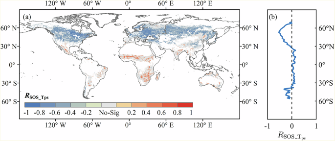
Significance was set at p < 0.05. a Spatial distribution of ({R}_{{sos_}{T}_{{ps}}}). Gray areas represent non-significant areas. b Latitudinal variations of the significant ({R}_{{sos_}{T}_{{ps}}}) averaged by each 1°-latitude.
At the latitudinal scale, a negative ({R}_{{sos_}{T}_{{ps}}}) was found approximately from 25°N northwards, consistent with the northern temperate zone (Fig. 2b). A positive correlation was mainly observed from 25°N to 40°S, corresponding to subtropical and tropical zones. Towards the extreme south (from 40°S southwards), a negative correlation was found.
Optimal temperature and growing-season temperature
We used ({T}_{{opt}}) to elucidate the divergent responses of SOS to temperature. The average ({T}_{{opt}}) over the global vegetated area was estimated to be 18.8 °C ± 7.9 °C, with maximum values close to 30 °C mainly appearing over tropical regions and minimum values near 5 °C prevail at high latitudes and in mountainous regions (Supplementary Fig. 6). Here we further evaluated the spatial pattern of the temperature differences between ({T}_{{gs}}) and ({T}_{{opt}}) (ΔT = ({T}_{{gs}}) – ({T}_{{opt}})). A negative ΔT indicates that the seasonal air temperature for vegetation growth is below the optimal growing temperature (({T}_{{gs}}) < ({T}_{{opt}})). Conversely, a positive ΔT means that the seasonal air temperature exceeds the optimal growing temperature (({T}_{{gs}}) > ({T}_{{opt}})). Approximately 63.3% of the vegetated areas exhibited negative ΔT, primarily located in North America, Eurasia, and small occurrences in South America and southeastern Africa (Fig. 3a). In contrast, a positive ΔT was found in 35.2% of the vegetated areas, predominantly in Africa, India, Australia, and eastern South America. On the latitudinal scale, approximately from 60°N to 25°N, which almost coincides with the boreal and temperate zones, we observed that ({T}_{{gs}}) was consistently lower than ({T}_{{opt}}) by around 5 °C. Conversely, spanning from 25°N to 40°S, which corresponds to subtropical and tropical zones, ({T}_{{gs}}) slightly exceeded the ({T}_{{opt}}) by approximately 1.5 °C. Further south from 40°S, we observed a conversion again with ({T}_{{gs}}) falling below ({T}_{{opt}}). This latitudinal variations in ΔT aligned with the latitudinal variations in ({R}_{{sos_Tps}}), suggesting that higher temperature led to earlier SOS when the ΔT was negative, but delayed SOS when ΔT was positive (Fig. 2bvs. Figure 3b).
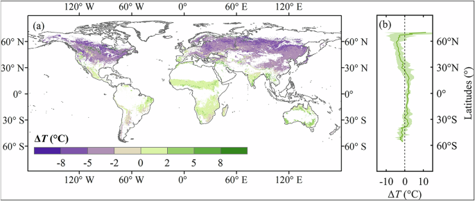
a Spatial distribution of the ΔT. b Latitudinal variations of ΔT averaged by each 1°-latitude.
Impacts of ΔT on ({{{boldsymbol{R}}}}_{{{boldsymbol{SOS}}}{{rm{_}}}{{{boldsymbol{T}}}}_{{{boldsymbol{ps}}}}})
We further analyzed the spatial variations of ({R}_{{SOS_}{T}_{{ps}}}) for regions associated with positive ΔT (ΔT > 0) and negative ΔT (ΔT < 0) over the 1982–2015 period. Figure 4a shows that SOS responded negatively to ({T}_{{ps}}) in most of the regions with negative ΔT, while positively to ({T}_{{ps}}) in regions with positive ΔT. Specifically, in 84.2% of the regions where ΔT < 0, ({R}_{{SOS_}{T}_{{ps}}}) was negative, with 61.6% showing significance at p < 0.05 level (Fig. 4b). The negative correlations between SOS and ({T}_{{ps}}) were strong and stable around -0.6 for a ΔT range of −9°C to −5°C. However, as ΔT from −5°C approaches 0 °C, i.e., when ({T}_{{gs}}) gets closer to the ({T}_{{opt}}), the influence of temperature on SOS becomes less pronounced, as evidenced by the increase in ({R}_{{SOS_}{T}_{{ps}}}) values from -0.57 at ΔT = −5 °C to −0.10 at ΔT = 0 °C (Fig. 5b).
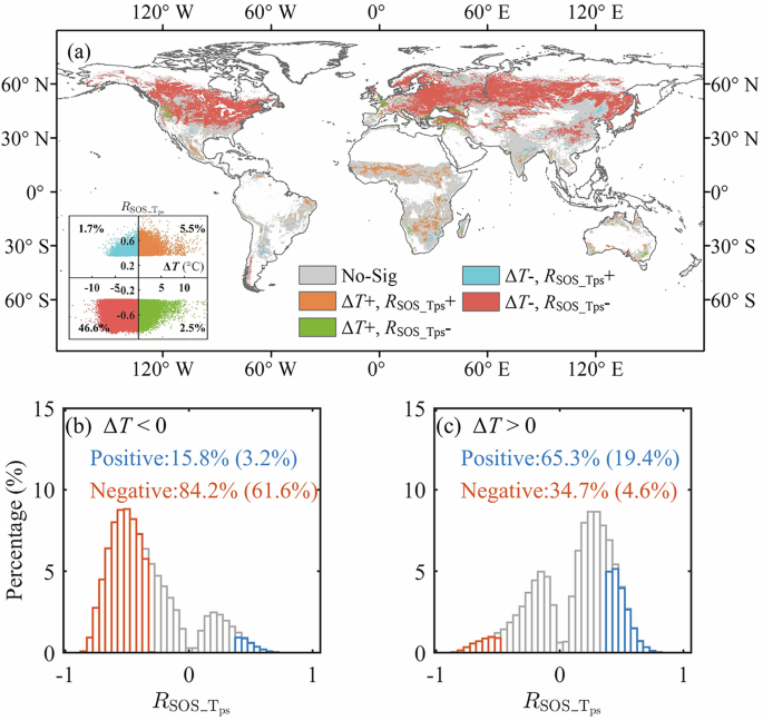
a Spatial distribution of relationships between ΔT and ({R}_{{SOS_}{T}_{{ps}}}). The insert scatter plot shows the overall distribution of relationships between ΔT and ({R}_{{SOS_}{T}_{{ps}}}), with each point representing a spatial unit on the map. Histograms of SOS trends in two climatic scenarios, where ΔT is positive (b) and ΔT is negative (c). Orange represents significant negative ({R}_{{SOS_}{T}_{{ps}}}); while blue represents significant positive ({R}_{{SOS_}{T}_{{ps}}}). The absence of near-zero correlations is explained by the fact that we derived the duration of pre-season based on maximum correlations between SOS and climatic variables (see Materials and Methods).
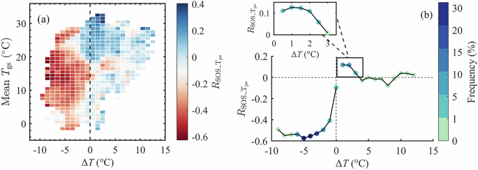
a({R}_{{SOS_}{T}_{{ps}}}) in different ΔT and mean annual growing-season temperature (({T}_{{gs}})) bins. Each climate bin is defined by 1 °C intervals of ΔT and mean annual ({T}_{{gs}}) between 1982 and 2015. The dashed line in (a) represents the climate condition when ΔT = 0. b Spatial variations of ({R}_{{SOS_}{T}_{{ps}}}) with gradients of ΔT. ΔT is divided into bins of 1 °C each. The colors represent the pixel density. The dashed lines in (b) represent the climate condition when ΔT = 0 and ({R}_{{SOS_}{T}_{{ps}}}) = 0, respectively. The inset sub-plot depicts the spatial variations of ({R}_{{SOS_}{T}_{{ps}}}) within the ΔT range of 0 °C to 3°C. Here, ΔT bins are defined at 0.5 °C intervals.
Conversely, in regions where ΔT > 0, ({R}_{{SOS_}{T}_{{ps}}}) was primarily positive (65.3% of ΔT > 0 regions), with 19.4% significant at p < 0.05 level (Fig. 4c). The significant positive correlations were primarily in areas between 25°N and 40°S. (Fig. 4a). Nonetheless, we still observed that 4.6% of ΔT > 0 regions exhibited significant negative ({R}_{{SOS_}{T}_{{ps}}}). These pixels were predominantly concentrated in regions with mean ({T}_{{gs}}) ranging from 15°C to 20°C (Fig. 5a). These areas include western North America, western Europe, southwestern Africa, and southern Australia (Fig. 4a). Within regions experiencing positive ΔT, the positive correlations between SOS and ({T}_{{ps}}) weakened from 0.12 to 0.00, as ΔT increased from 1 °C to 3 °C. This signifies a diminishing role of temperature in impacting SOS changes when ({T}_{{ps}}) exceeds ({T}_{{opt}}) and continues to diverge from ({T}_{{opt}}). The spatial patterns of ({R}_{{SOS_}{T}_{{ps}}}) variations for areas with ΔT exceeding 3 °C were inconclusive due to the limited number of pixels.
Discussion
The earlier shift of SOS in boreal and temperate ecosystems over the past three decades, along with global warmin,g has been well documented15,20,30. Our study confirms that SOS negatively responded to higher ({T}_{{ps}}) (i.e., earlier SOS with increasing ({T}_{{ps}})) in boreal and temperate ecosystems during the 1982-2015 period. Meanwhile, we also noted prevalent delayed SOS in subtropical and tropical ecosystems, and SOS positively responded to warmer ({T}_{{ps}}) (Fig. 1 and 2). Although ({P}_{{ps}}) and ({R}_{{ps}}) also contribute to regulating SOS shifts, their influences were less pronounced compared to ({T}_{{ps}}) (Supplementary Fig. 2). The temporal changes in precipitation exhibit irregularities and larger fluctuations, making the relationship between SOS and precipitation elusive31. Radiation may affect the SOS changes, but the magnitude of the effect is generally minor32, given the minimal temporal variability in radiation. In our study, we revealed that only a small portion of vegetated areas, notably 15.8% and 18.4% of the vegetated areas, displayed statistically significant relationships between ({P}_{{ps}}) and ({R}_{{ps}}) with SOS (Supplementary Fig. 2), respectively. In contrast, ({T}_{{ps}}) explained temporal variations in SOS in a substantially larger portion of the vegetated areas (51.7%).
To explain the divergent responses of SOS to warming, we introduce ({T}_{{opt}}) and(quad {T}_{{gs}}), of which the difference serves as a critical environmental variable for explaining the ({T}_{{ps}})-SOS relationship. We show that rising temperature led to an earlier SOS in the regions where ({T}_{{gs}}) is lower than ({T}_{{opt}}), whereas warming delayed SOS in the regions where ({T}_{{gs}}) exceeds ({T}_{{opt}}). Note that the SOS in this study was defined as the date when NDVI first exceeds 50% of seasonal satellite NDVI amplitude in the green-up phase (see Materials and Methods), rather than the leaf onset for plants. The SOS derived from satellite data using 50% threshold typically occurs later than the timing of leaf onset, which makes the SOS strongly affected by the photosynthesis and growth rate during the growing season. Generally, photosynthesis is most efficient at temperatures around ({T}_{{opt}}). Rising temperature towards the optimum increases the rate of enzymatic processes involved in photosynthesis33. This increased efficiency can accelerate vegetation growth, leading to an earlier SOS. In contrast, when ({T}_{{gs}}) exceeds ({T}_{{opt}}), increasing temperature directly influences photosynthetic process, making vegetation encounters a decline or inhibition in photosynthetic rate with warming due to decreased Rubisco enzymatic activity, which can potentially result in delayed SOS. Although water availability primarily limits SOS changes in subtropical and tropical ecosystems (Supplementary Fig. 9), temperature also has indirect impacts on photosynthesis via water cycle. First, elevated air temperature does limit canopy photosynthesis by controlling stomatal closure as a higher temperature usually comes with a higher vapor pressure deficit (VPD)34. Second, increased temperatures accelerate soil water evaporation, reducing soil moisture content. In water-limited ecosystems, reduced soil moisture availability can restrict plant water uptake, which in turn impairs photosynthesis35. Third, warming-induced water stress could suppress canopy photosynthesis through partial hydraulic failure (hydraulics) by cavitation36. These imply that plants in subtropical and tropical ecosystems, which are primarily limited by water availability, do not benefit from warming. Instead, they may even experience heat stress or photosynthetic inhibition, thereby resulting in delayed SOS. Therefore, the impacts of ({T}_{{opt}}) and ({T}_{{gs}}) on photosynthetic capacity can modulate the responses of SOS to warming.
It is unclear whether SOS will continue to occur earlier with future global warming. Many phenology studies have observed linear trend of earlier SOS with increasing temperatures in boreal and temperate ecosystems of NH37,38,39. However, some studies also suggested that SOS responses to climate warming may be nonlinear2,40,41, specifically, the response of SOS to warming may become less pronounced. Some existing explanations have been explored, such as the divergent responses to daytime and nighttime warming42, co-limitations of chilling and forcing13, or decreasing effects of increasingly high temperature43. Our study provides a potential explanation for the changes in SOS responses to warming. A space-for-time substitution in which observed spatial gradients are translated into temporal changes leads to the rudimentary prediction that the trend of earlier SOS will weaken as temperature rises towards ({T}_{{opt}}). When rthe ising temperature exceeds ({T}_{{opt}}), the response of SOS to warming will reverse to positive responses (i.e., warming delayed SOS). It suggests a potential future where delays in SOS become more widespread, while earlier shifts in SOS occur to a lesser extent.
Given the joint control of ({T}_{{gs}}) and ({T}_{{opt}}) on the responses of SOS to temperature, we suggest that ({T}_{{opt}}) should be considered in phenology models. This integration contributes to reducing uncertainties in phenology projections and simulations of land-atmosphere interactions under ongoing climate warming. Currently, many models rely on fixed temperature thresholds as a switch to control the timing of phenology events2. These models may overestimate the shifts of earlier SOS in boreal and temperate ecosystems with ongoing climate warming if the ({T}_{{opt}}) controlling is ignored. Our findings suggest that SOS responses to temperature are more complex and depend upon the difference between ({T}_{{gs}}) and ({T}_{{opt}}). Ignoring the ({R}_{{sos_}{T}_{{ps}}})– ΔT relationship, especially when ({T}_{{gs}}) goes beyond ({T}_{{opt}}) under future warming scenarios, can lead to inaccuracies in predicting SOS changes. The prediction of SOS changes associated with climate warming has considerable effects on ecosystem structure and function. Shifts in SOS can lead to cascading impacts on biodiversity. For instance, it can affect the synchrony between plant phenology and the life cycles of dependent species, such as herbivores, pollinators, and migratory birds, which rely on specific timing for food availability9,44. If further global warming causes the earlier shifts in SOS to decelerate or even reverse in the future, many interacting species may shift their life cycles at different rates or in varying directions, further disrupting this synchrony45. Such changes could alter species interactions and potentially impact community composition and ecosystem resilience. Additionally, SOS serves as a crucial indicator for food production, as it is closely linked to optimal sowing times. Shifts in SOS can disrupt traditional agricultural practices, potentially leading to reduced yields and compromised food security46. By utilizing phenological time windows (Greenup to Dormancy) for yield prediction, it can not only improved model accuracy but also facilitated earlier and more reliable crop forecasts47. Furthermore, many studies have demonstrated that global warming initially benefits greater ecosystem CO2 uptake by extending the carbon uptake period due to earlier SOS30,48,49. Our results suggest that as ({T}_{{gs}}) approaches and exceeds ({T}_{{opt}}) under climate warming, future rate of earlier SOS shift may decelerate or even reverse. Globally averaged surface air temperature over 2081–2100 is projected to rise by 0.2 °C–1.0 °C in the low-emissions scenario (SSP1-1.9) and by 2.4 °C – 4.8 °C in high-emissions scenario (SSP5-8.5) compared to the recent past (1995–2014)50. It implies that the increase in carbon uptake driven by earlier SOS may slow down or even stop in most regions in the future. Considering ({T}_{{opt}}) in phenology models could improve the accuracy of future predictions regarding SOS shifts and their consequences of global warming on ecosystems, including biodiversity, food production, and carbon cycling.
Our study highlights the importance of joint control of ({T}_{{gs}}) and ({T}_{{opt}}) on modulating SOS shifts under climate warming. By incorporating ({T}_{{opt}}) into models, we can potentially improve the accuracy of future predictions in SOS shifts and carbon cycle progress. However, it is worth noting that ({T}_{{opt}}) in our study was derived from historical satellite observations of NDVI at ecosystems and was assumed to be constant over time, which brings potential limitations. First, NDVI-based ({T}_{{opt}}), derived from ecosystem-level observations, may not directly capture the optimal temperature for specific leaf-level physiological processes like photosynthesis. For example, the ({T}_{{opt}}) values derived from more direct leaf-level measurements of photosynthetic parameters like ({V}_{{cmax}}) and ({J}_{max }) typically occur in 30–40 °C temperature range51. However, NDVI-based ({T}_{{opt}}) values at ecosystem-level are generally lower, mostly occurring in the range of 15–30 °C. The differences may originate from scale (leaf-level vs. ecosystem-level) and mechanistic responses. The ecosystem-level NDVI-based ({T}_{{opt}}) encompasses multiple ecological constraints such as canopy structure, water availability, and VPD. For example, under high-temperature conditions, increased atmospheric VPD and decreased soil moisture can induce stomatal closure, limiting photosynthesis and carbon assimilation at the ecosystem scale28. In contrast, leaf-level measurements of photosynthesis, used to determine the temperature response curve of ({V}_{{cmax}}) and ({J}_{max }) are usually conducted in absence of water stress. Additionally, we observed a dependence of NDVI-based ({T}_{{opt}}) on climate (e.g., NDVI-based ({T}_{{opt}}) in warmer climate was higher than that in colder climate), implying the acclimation process of vegetation at ecosystem-level. The acclimation process may change the shift the ({T}_{{opt}}) based on NDVI. By contrast, the mechanistic temperature dependence of ({{{rm{V}}}}_{{{rm{cmax}}}}) and ({J}_{max }) is a fundamental biochemical property and does not change with geography and long-term acclimation. Second, it is well-documented that plants possess the ability to thermally acclimate to changing climate conditions, suggesting the potential changes in ({T}_{{opt}}) over time as temperatures rise52,53. This thermal acclimation is also evident in the spatial pattern of ({T}_{{opt}}), as ({T}_{{opt}}) in warmer regions trends to be higher for vegetation growth than ({T}_{{opt}}) in colder regions (Supplementary Fig. 6b). The thermal acclimation of ({T}_{{opt}}) may alleviate the negative impact of future warming on SOS. Finally, it is imperative to consider the influence of other environmental factors on SOS shifts, such as precipitation and radiation. Global warming can impact precipitation patterns by modifying atmospheric circulation, which may lead to alterations in the timing, intensity, and distribution of rainfall. This is especially relevant in water-limited ecosystems where timely precipitation is essential for vegetation emergence. Similarly, global warming can influence radiation patterns by altering cloud cover, atmospheric composition, and seasonal photoperiod dynamics, further affecting SOS. The stronger effects of precipitation and radiation on SOS may make SOS shifts more complex and variable.
Materials and Methods
Climate datasets
Gridded monthly precipitation, air temperature, and radiation data for 1982 to 2015 were obtained from the ERA5-Land monthly averaged data, developed by the European Centre for Medium-Range Weather Forecasts (ECMWF), with a spatial resolution of 0.1°. The air temperature, converted from Kelvin (K) to Celsius (°C), is the temperature at 2 m above the land surface. The radiation data, which we transformed from Joules per square meter (J m-2) to kilowatt-hours (kW·h), is the monthly averaged amount of solar radiation (also known as shortwave radiation) reaching the earth surface. The precipitation, in mm/day, was aggregated to monthly totals (mm/month). Besides the ERA5 dataset, we also utilized the Climate Hazards Group Infrared Precipitation with Stations (CHIRPS) dataset over the same period (1982–2015) to further assess the robustness of the correlations between SOS and climatic variables. Compared to ERA5, a reanalysis dataset built primarily on model simulations with observations, CHIRPS integrates infrared satellite observations to provide more accurate precipitation estimates in areas with sparse ground-based weather stations54. However, its spatial coverage is limited to the region between 50°S and 50°N. Therefore, the main results shown in this paper are derived from the globally comprehensive ERA5 dataset.
NDVI dataset and pre-processing
We utilized the third-generation NDVI3g from the GIMMS group which provides a long-term dataset to derive the vegetation phenology spanning from 1982 to 2015. The GIMMS NDVI was generated at the spatial resolution of 8 km with approximately 15-day (two composites per month) temporal resolution. For data quality control, we excluded pixels identified as cloud-covered or snow-covered based on the product quality flags in the NDVI dataset. Subsequently, the resulting missing values were filled by linear interpolation. To suppress noise due to aerosols and solar elevation angles, we smoothed the NDVI time series with the Savitzky-Golay (SG) filter. The half-width of the smooth window was set to 4, and a third-degree polynomial was used for fitting. Additionally, 20 iterations were employed. To match the spatial resolution of climate datasets, we resampled the NDVI data to a spatial resolution of 0.1°.
Retrieval of the vegetation phenology
To focus on the areas with vegetation and clear seasonality, we applied the following criteria to exclude certain pixels. First, sparse vegetation and deserts were excluded by filtering out areas with a mean annual NDVI value lower than 0.115,25. Second, pixels with a mean coefficient of variation (CV) of the NDVI values during a year less than 0.1 were excluded as the growing season in these pixels cannot be optically retrieved55. Last, to further ensure the suitability of pixels for phenology extraction using NDVI in this study, we incorporated the European Space Agency Climate Change Initiative (ESA CCI) Land Cover (LC) product to remove bare areas and areas with sparse vegetation and evergreen forest cover. Moreover, the irrigated cropland areas were also removed from this study, as for those areas phenology may have a less direct link to climate due to human activities. To minimize the potential effects of land-cover type changes on phenology analysis, we specifically focused on pixels with consistent land-cover types throughout the period from 1992 to 2015, as determined by the long-term CCI-LC product. The global land cover types are shown in Supplementary Fig. 8.
Our analysis focused on vegetation areas exhibiting a distinct single growing season. Thus, we excluded vegetated areas with bimodal or multimodal NDVI seasonality from this analysis. We first employed a two-year window size to average the NDVI time series and to obtain a mean two-year NDVI curve for each pixel, considering that growing cycles in some areas can span two calendar years. Vegetated areas exhibiting bimodal or multimodal seasonality were then identified based on following criteria: (a) the presence of four or more peaks in the average NDVI curve, (b) the NDVI values from the peaks all exceed the mean NDVI, and (c) the valleys among the peaks should be lower than the mean two-year NDVI.
Considering that vegetation growing cycles vary greatly across the world and that the vegetation growing season in the Southern Hemisphere (SH) and Northern Hemisphere (NH) are opposite, we extended the annual NDVI time series by half a year in both directions (before and after) for each calendar year. This method was employed to ensure at least one full growing season cycle of vegetation for each studied calendar year. As an illustration, two sample points representing NH and SH were randomly extracted to present the extraction of phenology metrics from the NDVI time series (Fig. 6). To accurately retrieve SOS, the NDVI time series were first interpolated to daily temporal resolution after applying SG filter. We then used the local peak values, and the valley values in the NDVI curve to extract the vegetation green-up and senescence phases in each corresponding year. We used a minimum distance criterion of 250 days between each peak (or valley) to fit a whole length of the growing season, requiring the corresponding peak NDVI values (or valley NDVI values) to exceed (or fall below) the mean annual NDVI. Additionally, only when the valley points were recognized both before and after the peak point, the time series regarded as including a complete growing cycle of the current year. As shown in Fig. 6, a threshold of 50% was employed to extract both the SOS and the end of the growing season (EOS). The 50% threshold was selected in this study because that it is commonly used55,56,57 and generally corresponds to the moment of greatest increase in greenness58. Moreover, the 50% threshold is robust to noise and variability in NDVI time series, making it effective in regions with complex vegetation dynamics. SOS was defined as the date when NDVI first exceeds 50% of seasonal NDVI amplitude during the green-up phase. Similarly, EOS was defined as the date when NDVI first falls below 50% of the amplitude in the senescence phase. The amplitudes of the green-up and senescence phases may be different because the green-up and senescence valley values may differ. For this study, the EOS was only used to determine the vegetation growing season duration, a parameter used in the calculation of ({{{rm{T}}}}_{{gs}}), given that the purpose of this study was to understand the global responses of SOS to temperature.
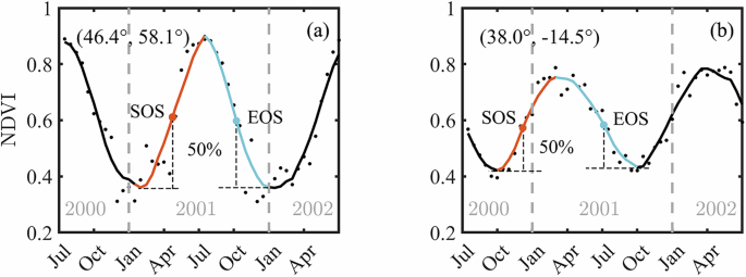
a An example of NDVI time series in the northern hemisphere. b An example of NDVI time series in the southern hemisphere. Based on minimum and maximum NDVI values, a 50% amplitude threshold is applied to retrieve the start of the growing season (SOS) and the end of the growing season (EOS). Black dots denote the raw NDVI, and solid lines represent the filtered NDVI. The orange and blue lines indicate the green-up and senescence phrases, respectively. The grey dashed lines in Fig. 6 represent divisions of each calendar year.
Calculation of the optimal temperature
Building on the methods for defining ({T}_{{opt}}) outlined in28, we determined ({T}_{{opt}}) for vegetation growth by examining the temperature response curve of GIMMS NDVI (Supplementary Fig. 7). Firstly, to maintain a consistent temporal resolution, the 15-day NDVI and monthly temperature were both interpolated to daily resolution. Subsequently, for each pixel, we grouped the temperature data into 1 °C temperature bins and grouped the corresponding daily NDVI throughout the entire study based on the temperature bins they fell within. The 90th percentile of the NDVI data with each temperature bin was defined as the response of NDVI to further remove outliers and natural variability due to other potential influences than temperature, such as clouds. Afterward, the moving averaged values of three temperature bins were calculated to develop the temperature response curve of NDVI. The ({T}_{{opt}}) was determined as the temperature at which NDVI was maximized. Additionally, the mean ({T}_{{gs}}) was calculated by averaging the daily temperatures during the growing season from 1982 to 2015. The SOS and EOS were utilized to determine the growing season duration.
Analysis
To identify temporal trends in SOS, we employed simple linear regression at each pixel. Given that precipitation, radiation, and temperature may all have effects on SOS variability, we performed per-pixel partial correlation analyses to isolate the effects of precipitation, radiation, and temperature on SOS variations over time. Since SOS variability highly associated with the climatic variables in the preceding months24,59, we analyzed the impacts of pre-season climatic variables on SOS changes. To determine per-pixel the optimal length of the pre-season for which accumulated precipitation, accumulated radiation, and average temperature had the largest influence on SOS changes, we calculated the partial correlation coefficients between SOS and these three climatic variables (i.e., ({T}_{{ps}}), ({P}_{{ps}}), and ({R}_{{ps}})) during the 1, 2, and 3 months preceding the month of multiyear averaged SOS over 1982-2015, respectively (Supplementary Figs. 3 and 5). Here, we constrained the pre-season length to be lower and equal to three-months, in analogy with previous studies that found that the length of the pre-season for vegetation responses to climate does generally not exceed this time window60,61. Based on the various pre-season lengths we used ERA5 data to extract the pre-season climatic variables. In addition, we employed CHIRPS-precipitation data in place of ERA5-precipitation to assess the robustness of the partial correlation between SOS and climatic variables. During the statistical analysis process, to more accurately estimate the proportion of different categories within vegetated areas, we computed the actual areas occupied by specific category instead of simply counting the number of pixels. Specifically, we calculated the actual land cover areas at a 0.1° spatial resolution for each latitude band. This is necessary because the conversion from geographical coordinates (like latitude and longitude) to projected coordinate systems can distort area measurements, particularly at higher latitudes. For example, actual land cover areas represented by each pixel (or grid cell) become smaller toward the poles in geographical coordinates. This distortion can be considerable when simply counting the frequency of pixels, leading to inaccurate estimates of actual land cover extent.
Reporting summary
Further information on research design is available in the Nature Portfolio Reporting Summary linked to this article.


Responses