Multidecadal drought impacts on the Lower Colorado Basin with implications for future management

Introduction
Megadrought conditions in the Colorado River Basin (CRB; Fig. 1a) over the past two decades associated with climate change1 have resulted in Lakes Powell and Mead, the two largest reservoirs in the US, dropping from 90% of capacity in Jan 2000 to a record low at ~25% of capacity in Nov 2022–Mar 2023 before rebounding slightly to ~35% after inflows in mid 2023–2024 (Supplementary Table 2). The main contributors to the declining reservoirs were Lower Basin overuse and declining Colorado River flows during 2000–2023 (15.4 km3/yr 12.5 million acre feet/yr, maf) at ~18% below the 20th century average (Supplementary Table 6)2,3. Current U.S. annual allocations of the Colorado River total 18.5 km3 (15 million-acre-feet [maf]), including 9.2 km3 (7.5 maf) each in the Upper and Lower basins. The Lower Basin allocation is divided up into 59% to California (5.4 km3, 4.4 maf), 37% to Arizona (3.5 km3, 2.8 maf), and 4% to Nevada (0.4 km3, 0.3 maf). By the 1944 treaty the US is obligated to deliver another 1.85 km3 (1.5 maf) to Mexico each year. Allocations are based on a 1922 Compact, federal laws, a Supreme Court decree, and the treaty with Mexico (including Minute 323), which collectively overallocate the river.

This map illustrates the Upper and Lower Colorado River Basin, along with naturalized flow at Lees Ferry (km3/yr, 2002–2024, Supplemental Table 6), mean annual precipitation (P, km3/yr; 2002–2024; Supplementary Table 3b), runoff (Roff, km3/yr 2002–2024; Supplementary Table 5b), surface water (SW) and groundwater (GW) water withdrawals (WW) (km3/yr, 2000–2020, Supplementary Table 11). The Active Management Areas that receive CAP water (Phoenix, Pinal, and Tucson) are indicated, highlighting key groundwater management regions. Two cross sections are presented: A–A’ in the upper right and B–B’ in the lower right illustrate topographic and geological variations across the Plateau and alluvial basin physiographic provinces of the Lower Basin57.
Colorado River management agreements expire in 2026, including the 2007 Interim Guidelines and the 2019 Drought Contingency Plans. Thus, the seven states and 30 tribes that share the Colorado River, along with the federal government and Mexico, are currently negotiating new rules that will govern the operation of reservoirs post 2026. Among other outcomes, these new rules will dictate the conditions under which the Secretary of the Interior will declare shortage conditions in the Lower Colorado River Basin (LCRB). Arizona represents ~70% of the LCRB land area and includes 22 out of the 30 Indian Tribes (generally with reserved rights to water supply from Arizona’s allocation, 1908 Supreme Court Decision). Arizona is particularly vulnerable to Colorado River water shortages declared in the LCRB because of reliance on the Central Arizona Project (CAP) canal (530 km long) which delivers 57% of Arizona’s Colorado River water entitlement (2.0 out of 3.5 km3 allocated (1.6/2.8 maf) into central Arizona, including Phoenix, Pinal, and Tucson areas. Central Arizona is junior in priority to all California uses and also junior to Arizona Colorado River diverters along the Colorado mainstem above Yuma, including Fort Mojave and Colorado River Indian Tribes4. CAP water deliveries are critical to sustainable water management in Central Arizona, which has little or no access to renewable surface water (SW) supplies but large quantities of groundwater (GW)5.
Water management in the CRB has evolved over the past century with some of the major agreements described in Supporting Information (SI), Section 3. There are many parallels between water management in the CRB and in the California Central Valley6, with GW depletion in the early to mid-1900s followed by stabilization of GW levels in many regions with SW imports (Central Valley and State Water Projects and CAP aqueduct). Both the CRB and the Central Valley use SW transfers to support switching from GW to SW irrigation (termed GW Savings Facilities [GSFs] in Arizona and ‘in lieu recharge” in California) and managed aquifer recharge (MAR) using spreading basins (termed Underground Storage Facilities [USFs] in Arizona)6,7. Because of the high cost of the CAP aqueduct (~$5 billion) and inability of agriculture to repay it’s expected share of those costs to the Federal Government, irrigators in Central Arizona gave up their contractual water rights to municipalities and Native Americans and therefore are most vulnerable to shortages8. In addition, the much lower cost of GW pumping in Arizona relative to treatment and delivery of CAP water resulted in a “pump and replenish” paradigm where GW continued to be pumped and was later replenished by CAP renewable SW recharge of depleted aquifers, often at a location distant to the pumping9,10. One recent example shows that the estimated costs of constructing and operating a SW treatment plant to use Colorado River water directly was ~1000 times more expensive than pumping GW and replenishing it using MAR based on spreading basins (SI, Section 3). The first ever shortages in the LCRB were declared in 2022 and 2023 resulting in less direct (MAR) and indirect recharge (GW savings facilities and additional incidental recharge from SW irrigation)11, highlighting the difficulty of replenishing pumped GW when reductions in Colorado River CAP deliveries occur.
Many previous studies have been conducted on hydroclimatic issues in the CRB, ranging from snow studies in the UCRB12, climate extremes/change impacts13, megadrought conditions14, and SW accounting15. The UCRB accounts for about 85% of the surface flow in the basin and has been impacted by long-term climate trends, as shown by variability in precipitation and runoff (Supplementary Tables 3–6). Warming and drying trends could have greater impacts on Colorado River flow than currently assumed with possible additional flow declines of up to 20% by mid-century1,13.
A detailed SW budget of the basin revealed the dominance of irrigated agriculture in the region, with irrigated cattle feed crops accounting for 46% of all direct water consumption from 2000 to 2019 whereas municipal, commercial, and industrial sectors accounted for 18% of total water use15. Data on annual consumptive uses and losses were compiled by the Bureau of Reclamation16,17. Previous studies of terrestrial total water storage (TWS) data from the Gravity Recovery and Climate Experiment (GRACE) satellites tracked changes during 2002–2015 and attributed the TWS declines to reductions in reservoir, soil moisture, and GW storage18,19. GW-level trends were analyzed from monitoring data in previous studies20. A total of ~70 aquifers were mapped in the Basin and Range province in the LCRB that extend to depths of up to 3 km (Fig. 1c, Fig. S2). Regional GW flow models have been developed for most of the highly exploited aquifers in the Lower Basin21,22,23. Depletion of GW was estimated to be 105 km3 from 1900 to 2008 based on GW models and GW level monitoring data24. Widespread subsidence and fissuring were recorded in many of the GW basins in the LCRB linked to aquifer overexploitation and more recently based on Interferometric Synthetic Aperture Radar (InSAR) data25.
The objective of this work was to conduct a comprehensive assessment of past and current water resources accounting, linking climate, SW, and GW to help guide future management strategies in light of likely future shortages on the Colorado River. The analysis focused on the LCRB; however, water from the UCRB feeds the LCRB and data for the UCRB are provided for context. This study differs from many previous studies in comprehensively assessing a wide variety of data sources, including data on TWS anomalies (TWSAs) from GRACE satellites, monitored reservoir storage, modeled soil moisture storage, GW level monitoring, regional GW modeling, subsidence data from InSAR satellites, and water budget accounting from state agencies. This study differs from a recent SW budget accounting and crop water use study15 in considering GW systems and using a wider variety of data sources. Harmonizing the various data sources in this study should provide a detailed understanding of the linkages and feedbacks between climate and water resources management and improved assessment of strategies toward more sustainable management in the future. The results of this analysis should provide a much deeper understanding of the interactions between SW and GW to assist water managers in successfully navigating the challenges of decadal drought, climate change, renegotiation of reservoir operating rules, and competing uses in overallocated river and aquifer systems. Renegotiation of water management agreements for post 2026 operations highlights the timeliness of this work.
This paper proceeds as follows. Section 1, Introduction, sets the stage for this effort including some of the key policy issues. Section 2, Results, provides information about how the ongoing drought has impacted a number of key water metrics. These metrics are Water Storage and Variability and Water Use, and GW Level Monitoring, Regional GW Modeling and Subsidence). Section 3, Discussion, provides commentary on Adaptation to Climate Extremes and Water Scarcity and Implications for Future Water Management. Section 4 provides overall Conclusions. Section 5 covers Methods including data sources. The Supplemental Information provides data source locations and links, acronyms, water governance, aquifers, and additional figures and tables.
Results
The UCRB has higher precipitation and runoff than the LCRB with Lees Ferry at the boundary between the two and naturalized flow averaging 15.8 km3/yr (2002–2024) corresponding to the GRACE period (Fig. 1 map, Supplementary Table 6). Geologic cross sections show the Colorado Plateau (Fig. 1), including Mesozoic sedimentary rocks underlain by Paleozoic sandstone and carbonates and crystalline bedrock and alluvial basins (Fig. 1). A total of 71 aquifers have been delineated in the LCRB that are up to 3 km deep, bounded by faults, and filled with sediments underlain by sedimentary and volcanic rocks and crystalline bedrock (Fig. 1B-B’).
Water storage variability
GRACE data show that TWS declined less in the UCRB (11 km3) than in the LCRB (45 km3) over the 22.2 yr period from the beginning of GRACE data in April 2002 through June 2024 (Fig. 2c, Table 1). The large depletion in the LCRB exceeds the capacity of Lake Mead (~32 km3) by ~40%, the largest reservoir in the US. There is substantial interannual variability with TWSA in the UCRB that is correlated with the drought index from the US Drought Monitor (USDM; R = 0.80) (Supplementary Table 8b). The UCRB shows drought in the early 2000s followed by shorter droughts after 2010. TWSA variability is also linked to precipitation with peaks in 2005, 2010, 2015, 2019 and rising in 2023 (Supplementary Table 3a). The relationship between TWSA and UCRB snow water equivalent is also evident with highest snow values in 2017, 2019, and 2023 (Fig. 2a). Similar patterns are found in runoff in the UCRB, peaking in 2005, 2011, 2017, 2019, and 2023 (Supplementary Table 5a). The drought pattern in the LCRB is similar to that in the UCRB but more persistent through time showing gradual TWS decline after 2011 with partial recovery in 2023 (Fig. 2b). The correlation between GRACE and USDM data is less in the LCRB (R = 0.68) than in the UCRB (Supplementary Table 8b). Linkages between TWSA and precipitation are also more subdued in the LCRB and runoff is very low and temporally invariant in the LCRB (Supplementary Table 5a). Long-term naturalized discharge at Lees Ferry between the UCRB and LCRB shows large interannual variability over the past several decades (Fig. 2b).
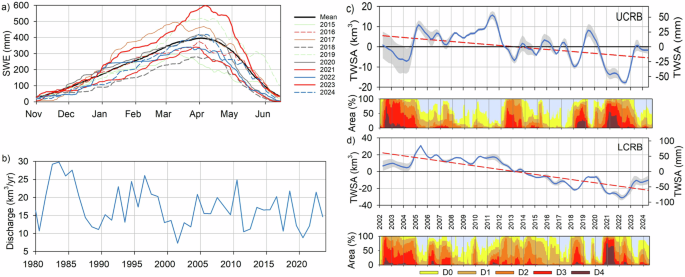
a Snow water equivalent variability in the recent 10-year period (2015–2024) (Supplementary Table 4), b naturalized discharge at Lees Ferry on the Colorado River between the UCRB and LCRB (Supplementary Table 6), and c, d GRACE Total Water Storage Anomaly (TWSA) in the UCRB and LCRB (Supplementary Table 7) and US Drought Monitor intensity (Supplementary Table 8). Linear trends in TWSA are shown by the dashed red line with trend values of −0.51 km3/yr in the UCRB and −2.0 km3/yr in the LCRB (Supplementary Table 10b). There is substantial interannual variability with TWS in the UCRB remaining fairly stable through 2011, declining sharply to 2013 during intense drought, and then stable and rising in 2019 followed by a rapid decline in 2019–2022 with a return to pre-2021 levels in 2023–2024. (D0, abnormally dry; D1, moderate drought; D2, severe drought; D3, extreme drought, D4, exceptional drought).
Reservoir storage is dominated by Lake Powell in the UCRB and Lake Mead in the LCRB (Fig. S3b). The linear storage trend in Lake Powell totaled −4.9 km3 over the GRACE period (22.2 yr: 2002–2024) (Table 1). Storage declines were ~2× greater in Lake Mead, totaling −9.7 km3. The two reservoirs have been jointly managed since 2007 but storage time series in the two reservoirs are poorly correlated (r = 0.4), a not unexpected result given the reservoir management rules. Soil moisture storage change based on GLDAS models during the GRACE period was greater in the UCRB (−5.7 km3, 22.2 yr period) than in the LCRB (−2.4 km3) (Table 1, Fig. S3c).
In the UCRB, the linear trend in TWS depletion (11.3 km3) over the GRACE period can be generally accounted for by changes in reservoir and soil moisture storage (summed linear declines 10.5 km3) suggesting minimal GW storage change (Table 1, Fig. S3). In contrast, in the LCRB, the linear trend in TWS depletion (45 km3) greatly exceeds the sum of reservoir and soil moisture storage depletion (~12.2 km3). The large residual (−27 km3) in the LCRB over the 22.2 year period likely reflects GW depletion from pumping and reduced recharge during drought (Table 1, Fig. S3d).
Water use
Water withdrawal or use (irrigation + municipal), including SW and GW, averaged 3.0 km3/yr (2.4 maf/yr) in the UCRB and 7.2 km3/yr (5.9 maf/yr) in the LCRB over the period of record (2000–2020), dominated by irrigation which accounted for 95% of total water use in the UCRB and 77% in the LCRB (Table 1, Fig. 3a). SW accounted for 98% of irrigation water in the UCRB whereas SW and GW contributed about equally to irrigation in the LCRB. The water use data are similar to the GRACE satellite data with no GW depletion in the UCRB consistent with SW-sourced irrigation. The analysis is more complicated in the LCRB with SW- and GW-sourced irrigation and differences between water use (diverted SW or extracted GW) and consumption (evapotranspired water). Water use has remained fairly stable over the past two decades in both the Upper and Lower Basins (Fig. 3b). SW irrigation in the UCRB is located along river valleys and in the LCRB is located along the mainstem Colorado River below Hoover Dam in Arizona and California (Fig. S1). Irrigation from SW and GW sources is also concentrated in the Phoenix and Pinal County areas in Central Arizona. Prior to the CAP, these Central Arizona areas were mostly supplied by GW pumping with the exception of some SW from the Salt River Project System (includes Verde River) in the Phoenix area and from the Upper Gila River in Pinal County. Other areas outside of Central Arizona have also had GW-dependent agriculture and in recent years some of this agriculture has expanded to take advantage of no limits on GW pumping (e.g., Riverview Dairy in Cochise County and Saudi Arabia farms in La Paz County)26,27,28. Irrigation efficiency (water consumption/water withdrawal) is generally low, ranging from 55 to 60% in both basins (Supplementary Table 11), mostly reflecting inefficient flood irrigation, which accounted for ~70% of irrigation in UCRB and LCRB in 2015 (Supplementary Table 12). The low irrigation efficiency indicates that as much as 35–40% of the water that is withdrawn from the source is returned to the Colorado River in the UCRB for rediversion, and recharges GW in the central part of the LCRB.
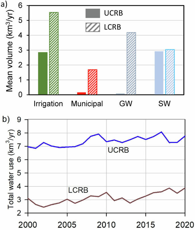
a Mean annual water volume (2000–2020) for irrigation and municipal sectors and corresponding water sources (GW groundwater, SW surface water) for the Upper and Lower Colorado River basins (UCRB, LCRB); b temporal variability in total water use (SW +GW withdrawals) in the UCRB and LCRB (Supplementary Table 11). Data source: USGS HUC 12 data.
Groundwater level monitoring
Analysis of GW level monitoring focused on the LCRB because GW use in the UCRB was limited and previous analysis suggested stable GW level trends19. GW levels are well correlated with GRACE GW storage in the LCRB (R = 0.94; Supplementary Table 13b) demonstrating the ability of GRACE to monitor regional GW storage. To convert GW levels to GW storage, GW levels need to be multiplied by the storage coefficient. A regional estimate of the storage coefficient or specific yield was based on the slope (0.11) of GRACE GW storage versus GW levels in the LCRB (Supplementary Table 13b) which is equivalent to an average specific yield of 11% across the LCRB aquifers that include alluvial basin aquifers and regional Paleozoic sedimentary aquifers across the Colorado Plateau (Fig. 1b).
GW level monitoring data (2000–2023) show large spatial variations in GW level trends in the different LCRB aquifer basins in response to water sources (GW, SW) and intensity of water use (Fig. 4). Some areas are characterized by high GW use with no access to SW (Fig. 4g) (e.g., Willcox and Douglas basins in the southeast), resulting in the largest decline in GW levels (cumulative ~11 m, 2000–2023). In contrast, in the Active Management Areas (AMAs: Phoenix, Pinal, and Tucson) that received Colorado River water through the CAP aqueduct, GW levels rose by an average of ~3 m (Fig. 4d). Areas of moderate GW use (GW use <recharge rates) are characterized by an average decline of ~3 m (Fig. 4b) Regions with predominantly SW use near the Colorado Mainstem also show minimal GW level change (Fig. 3c). The Plateau region (N Arizona, Little Colorado River Basin) occupies ~40% of the LCRB area but is minimally developed and shows limited GW level decline (~0.8 m) that is primarily attributed to reduced recharge during the recent multi-decadal drought (Fig. 4e). The GW level compilation represents average hydrographs from available data for each basin. The data were not spatially averaged and may be biased toward conditions in the most heavily monitored areas, which are also areas with the most wells and the most exploited.
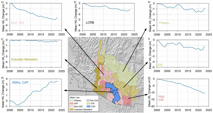
Trends in GW levels from monitoring data in the a overall LCRB extent, b regions with moderate or low GW usage (GW extraction<recharge rates), c regions near or dominated by the Colorado River, d AMAs (Active Management Areas) that receive Central Arizona Project [CAP] water, e Plateau region, f basins dominated by perennial streams (SW), and g GW-dependent regions where GW extraction exceeds recharge. Summary data are provided in Supplementary Table 13. The names of the subbasins in each category are provided in Supplementary Table 14.
It is difficult to estimate median water table depths in each basin because of large variability from basin edges to centers and over time. Reported median water table depths from 1891 to 2024 range from ~3 m in basins that are traversed by perennial streams to ~60 m in the AMAs to 120 m in the Plateau Region (Fig. S4).
Regional groundwater modeling
The regional GW models also provide information on changes in GW storage and other water budget components since the early 1900s; however, in this analysis we focus on 1940–2020 which includes the period with greatest depletion in the mid-1900s and is covered by regional models of all the major exploited GW areas (Fig. 5). The models were calibrated to monitored GW levels, stream baseflow, and estimated water-budget components. They repsresent the best estimates of GW storage change because of those constraints. The modeled aquifers represent about half of all of the aquifer area in the LCRB (Fig. S5). The main source of natural recharge in the region is infiltration along mountain fronts and stream losses, particularly flood flows. Recharge in the central Arizona basins also includes MAR, mostly from CAP deliveries that is discussed more in Section “Adaptation to climate extremes and water scarcity”. Incidental recharge should be accounted for and represents infiltration of excess irrigation (i.e., irrigation application that exceeds crop consumption) from SW and GW sources. Output from the aquifers is dominated by GW pumpage for irrigation, followed by baseflow to streams, and riparian ET (Fig. 5a). Storage trends varied across basins and over time (Fig. 5b). Pumpage of GW in all of the modeled aquifers totaled ~260 km3 (~210 maf; 1940–2020), about 4× greater than the aquifer storage depletion (~65 km3, ~53 maf) (Supplementary Table 15). The large difference between pumpage and storage depletion is attributed to capture related to stream leakage during the early period with perennial streams switching to ephemeral status, decreasing riparian ET with deepening GW levels, and increasing SW irrigation related to CAP.
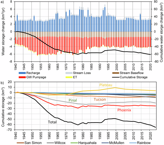
a Time series of GW budget components and cumulative GW storage change summed over all AMAs. b cumulative GW storage for each regional GW model (Phoenix, Pinal, Tucson, San Simon, Willcox, Harquahala, McMullen, Rainbow, Plateau). Data are provided in Supplementary Table 15.
The cumulative decline in GW storage varied over time and was greatest from the 1940s through mid-1970s as pumpage more than doubled from ~2.0 km3/yr in the early 1940s to an average of ~4.8 km3/yr in the 1950s through mid 1960s (Fig. 5a). Stabilization and slight increases in GW storage after this time reflect reduced pumpage (1980s–2010, ~2.7–3.3 km3/yr by decade), wetter periods in the late 1970s, early 1980s, and early 1990s as shown by almost doubling of recharge from an average of ~3.5 km3/yr in the 1940s through 1950s to 6.5–7.7 km3/yr during the wetter periods.
The modeled water budgets vary across the GW basins with the largest volumes in the Phoenix AMA, followed by the Pinal County area south of Phoenix (Fig. S6, Supplementary Table 15). Storage depletion in the Phoenix area occurred primarily from ~1940 to 1960, averaging ~1 km3/yr with pumpage peaking at 2.5–~3 km3/yr in the 1950s. This period was followed by fairly stable storage related to reduced GW withdrawals partially due to urbanization, increased recharge including from flood flows during late-1970s through late 1990s, and use of SW from the Colorado River (CAP) for MAR and replacement of GW irrigation beginning in the late 1980s. Similar results, but delayed trends with later SW deliveries, occurred in the Pinal County area with aquifer depletion occurring mostly from 1940 to mid 1970s. GW depletion in the Tucson area was much less than that in the Phoenix and Pinal county areas during 1940–2005. Significant CAP MAR began in Tucson in ~2000 which allowed the city to utilize its renewable Colorado River supplies through a GW pump and replenish scheme. GW models for aquifers outside of central Arizona show continuous depletion through present with lower magnitudes (Supplementary Table 15). Examples include GW depletion in Harquahala totaling ~3.0 km3 (1940–2020), McMullen: 4.7 km3, Rainbow: 2.4 km3; San Simon: 4.1 km3, and Willcox: 8.4 km3.
Simulated storage change in all of the models during 2002–2023 (−12.9 km3) represents only about 40% of the GW storage change from GRACE for this period (33.0 km3) (Supplementary Tables 13b and 15). Assuming the models are reasonably accurate representations of water budgets, the difference between GRACE and modeled GW storage change is attributed to storage loss in unmodeled basins. These unmodeled basins are not heavily exploited for GW resources; therefore, the unmodeled storage loss likely results primarly from reduced recharge during the drought. Much of the storage loss may have occurred in the Plateau and highland areas of central Arizona and western New Mexico. The simlutions for those areas did not include calibration to obserations after ~2010 and likely overestimate recharge rates during the drought.
The regional models were used to assess the reliability of the projected 100 yr Assured Water Supplies for Phoenix and Pinal AMAs within the context of all supplies and demands29,30. Results for the Phoenix AMA show projected depletion exceeds the 300 m (1000 ft) threshold depths or bedrock depths along the margins of the basin where the aquifer is thin. The unmet demands represent ~4% of the total demand over the projected 100 yr period (2022–2121). The agriculture sector represents ~26% of the total projected demand from all sectors. The modeled storage loss is ~48 km3 (~39 maf) with an average GW level decline of ~55 m (185 ft) across the AMA by 2121. In the Pinal AMA, agriculture is projected to be the dominant GW user (60% of total demand from all sectors) with projected unmet demand comprising ~10% of total projected 100 yr GW demand from all sectors. GW storage is projected to decrease by 34 km3 (27.5 maf) with an average GW decline of almost 100 m (~320 ft) across the AMA. Doubling the GW depth would double the pumping costs from energy required for increased lift, neglecting well deepening or changing pumps31. It is not clear if agriculture will be able to support the increased pumpage costs with declining GW levels. The increased GW storage loss in the projection period is attributed to increased pumping demand, moving from agricultural to urban sectors, decreased agricultural recharge, and reduced artificial recharge.
Subsidence
Overexploitation of GW induced aquifer-system compaction and land subsidence, which were extensive across many alluvial basins in the LCRB. For example, the Pinal AMA GW model simulated compaction ranging from ~15 to 20% of total GW storage depletion from the 1930s, indicating permanent loss of aquifer storage32. Long-term historical subsidence ranged from ~5.5 m in the western portion of Phoenix near Luke Air Force Basin (1957–1991), 4.9 m in Eloy, Pinal County (1952–2018), and 3 m in Willcox Basin (1969–2023) (Fig. S7).
Data from InSAR provide a regional picture of more recent subsidence (2010–2023) in the LCRB (Fig. 6, Supplementary Table 16). The Willcox basin (4950 km2 area) in southeastern Arizona showed the greatest net subsidence in the LCRB, up to 1.2 m in the area of maximum subsidence over the past ~15 years (2010–2024). GW level hydrographs near areas of maximum subsidence in the Willcox Basin ranged from 20–40 m. Earth fissures are also widespread in the Willcox Basin because of differential compaction associated with varying depths to basement rock, particularly near the margins of the basin25. Subsidence in San Simon Basin to the east of the Willcox Basin was also widespread, related to large GW level declines (≤~50 m). Intensive subsidence and fissuring in Willcox and San Simon basins are attributed to large GW level declines (20–50 m). Thick clays are mapped in the the internally drained Willcox Basin that has an ephemeral lake or playa towards the center and in San Simon Basin and represent the dominant compressible unit. There is no access to SW in either the Willcox or San Simon basins. Intensive subsidence with fissuring was also recorded in McMullen Valley northwest of Phoenix (0.9 m, 2010–2024), linked to large GW-level declines (≤~50 m), thick and extensive silt and clay, and lack of access to SW.
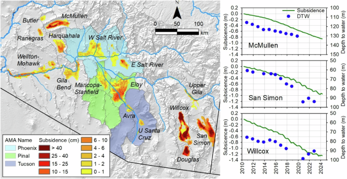
Map of land subsidence based on InSAR data from 2010 to 2023. Data for the Upper Gila (Safford Basin) and Lower Gila (Welton-Mohawk area) are only available for 2017–2021. Time series of subsidence trends and water-table depths on right in areas of maximum subsidence in McMullen, San Simon, and Willcox basins. Data are provided in Supplementary Table 16.
Recent subsidence in the remaining basins (Phoenix, Pinal, and Tucson) is mostly residual (0.1–0.3 m) and attributed to delayed drainage of thick compressible clays linked to historical GW depletion (Fig. 6). Subsidence was recorded near Scottsdale in the E Salt River Valley within the Phoenix area (up to ~0.2 m, 2010–2021). Reduction in CAP Colorado River SW deliveries for irrigation with the recent drought has resulted in a resumption of GW withdrawals in some regions which will likely cause renewed aquifer compaction and land subsidence. With reduced CAP Colorado River SW deliveries and resumption of GW withdrawals, future rates of land subsidence may be similar to those recorded prior to SW delivery in basins that continue to be dominated by irrigated agriculture. Urbanized agricultural areas should experience lower rates of land subsidence without SW deliveries compared to rates that occurred prior to urbanization. Inelastic GW storage depletion linked to subsidence is projected to be ~15% of total storage depletion in the Pinal AMA29. Aquifer compaction/subsidence was only considered in the Pinal AMA model; however, the Phoenix and Tucson AMAs have also experienced subsidence. Maximum subsidence rates in the agricultural areas of the Phoenix AMA are similar to those of Pinal AMA; therefore, subsidence could be a limiting factor in the Phoenix AMA also. Use of MAR has allowed Tucson to reduce GW withdrawals in the primary well field, minimizing GW level declines and subsidence. While water budgets have been projected for the next 100 yr in Phoenix and Pinal areas29,30, subsidence associated with projected depletion and impacts on infrastructure may limit future water availability.
Discussion
Adaptation to climate extremes and water scarcity
Various approaches have been deployed to resolve spatiotemporal disconnects between water supply and demand in the LCRB. Basic approaches include reducing demand (conservation), diversifying supplies, and storing and transporting water. Water demand reduction is seen in the regional GW models; annual irrigation pumpage decreased from a mean of 4.6 to 4.8 km3 (1940 to early 1950s) to 2.6 km3 (2010–2020) averaged over all of the modeled basins (Fig. 5). Irrigated agriculture declined in recent decades (2005–2020) by 17% (Tucson AMA, 2012–2020) and 25% (Phoenix AMA, 2005–2020)21,23. Voluntary fallowing programs have been noted in the LCRB23. Irrigation non-expansion areas have been established in Harquahala, Hualapai, and Joseph City to preclude any further increases in water withdrawal for irrigation. Douglas Basin was recently converted from irrigation non-expansion area to AMA status. Expansion of urban areas may be linked to water demand reduction because urban areas use less water on average per km2 than irrigated areas. The largest increase in urbanization was recorded in the Phoenix area, ~790 km2 (Supplementary Table 17), but much of the urbanization has been on vacant desert land, not existing irrigated agricultural land, which would increase GW pumping and overall demand33,34. Reductions in Phoenix AMA agricultural demand have been completely replaced by increased urban and industrial uses.
Additional renewable water supplies are extremely limited35. Wastewater has been reused for USFs and GSFs, totaling ~1.7 km3, mostly in the Phoenix area (1989–2019; Supplementary Table 18). However, much larger wastewater volumes have been used for other purposes (e.g., Palo Verde nuclear power plant cooling). Stormwater has also been captured in Arizona with over 50,000 dry wells installed in Phoenix36,37.
Water transport and storage are important mechanisms deployed to adapt to climate extremes and scarcity and reflect the interconnection between SW and GW as Colorado River water is transferred to Central Arizona and some stored in depleted aquifers. Transfers of Colorado River water through the CAP aqueduct began in 1985 totaling 0.44 km3 up to 1989 (Fig. 7). Arizona enacted laws to allow for the “banking” of Colorado River water in central Arizona aquifers to provide for future urban development, replenish municipal GW use, and mitigate against the impact of Colorado River shortages. Water banking in central Arizona occurs in two ways: through MAR spreading basins at “Underground Storage Facilities” (USFs) and through delivery of Colorado River water to irrigators who switched from GW to SW at “Groundwater Savings Facilities” (GSFs)7 (Fig. 7). The Arizona Water Banking Authority manages MAR in the majority of facilities11. The GW thus recharged at a USF and/or saved at a GSF becomes a “Long-Term Storage Credit” (LTSC) that conveys a legal right to pump GW that can be used or sold. LTSCs are routinely created, “recovered” (pumped back out), and sold. Cumulative net storage for 1989–2019 was 10.5 km3 (8.5 maf, 67% for USF and 33% for GSF) assuming 37% of GSFs recharge GW (Table 1, Fig. 7). LTSCs may overestimate water storage by a factor of ~1.7 as they assume 100% of the GSF increases GW storage (9.3 km3) whereas the GW models estimate that ~37% of the GSF recharges the aquifer (3.5 km3). Net cumulative incidental recharge that was non-GSF SW was 14.2 km3 (11.5 maf, 1985–2019), 35% greater than USF and GSF combined (Fig. 7). These data highlight the importance of incidental recharge from SW irrigation in the basin in addition to USFs and GSFs. The total of ~25 km3 represents ~5× the annual water demand in the central Arizona AMAs. This water accounting only reflects water transfers through the CAP, SW/GW switching, and waste water irrigation but excludes GW pumping for irrigation, municipal and industrial sectors; hence, the discrepancies between these volumes and those reported from GW modeling.
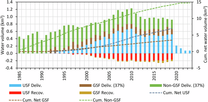
Water deliveries for Managed Aquifer Recharge (MAR) sites (USF) totaled over the Active Management Areas (Phoenix, Pinal, and Tucson AMAs). Water deliveries for agricultural use (GSF and non-GSF designated). USF underground storage facilities, GSF GW savings facilities, Deliv. Deliveries: 37% of deliveries are assumed to equal the incidental recharge rate, Recov. recovery, Cum. cumulative. Data are provided in Supplementary Table 18.
There are many parallels between the adaptive strategies used in Arizona to those deployed in California to address climate extremes and water scarcity6,7. GW overexploitation in California during the early to mid-1900s was partially addressed by water transfers from the humid North to the semiarid South through large aqueducts (Central Valley and State Water projects) and Colorado River water to southern California. California was required to reduce its annual use of Colorado River water from 6.4 km3 (5.2 maf) to 5.4 km3 (4.4 maf) once Arizona began diverting its allocation through the CAP. California accomplished this reduction through the 2001 Quantification and Settlement Agreement. This agreement relied extensively on transfers of Colorado River water from agricultural to urban uses to minimize harm to municipal users impacted by the 1 km3 (0.8 maf) reduction in Colorado River water deliveries. California also has a program to bank SW using spreading basins and in lieu recharge (switching from GW irrigation to SW irrigation). GW levels have partially recovered in many areas of California.
Implications for future water management
Analysis of historical data shows the value of different management strategies over the past three decades, particularly in the LCRB in Arizona; urbanization, replacement of some agricultural GW use with use of Colorado River water and related incidental recharge, and MAR combined to stabilize GW levels in central Arizona. Future GW levels will depend on the balance between water supplies, SW and GW, relative to demands and the ability to resolve spatiotemporal disconnects between supplies and demands. Future SW supplies will vary with climate extremes/change and regulations on Colorado River water distributions. Methods of potentially addressing the disconnects are addressed below.
About 85% of the Colorado River flow is derived from the Upper Basin. Therefore, climate and snow conditions in the UCRB are critical for determining SW flows in both the UCRB and LCRB. Pervasive drought conditions over the past couple of decades have been extremely challenging1,2. Projected supplies from the Colorado River are highly uncertain but most studies project future flow declines38. River discharge has decreased by ~9% per degree warming, which is attributed to increased ET linked to snow loss and reduced reflection from solar radiation13. Some studies project additional declines in Colorado River flow by 2050 ranging from ~10 to 20% relative to 2000–20201,13. However, a recent study indicates that precipitation, rather than temperature, is the primary driver of flow in the CRB, accounting for ~80% of decadal variability in historical flow at Lees Ferry (boundary between UCRB and the LCRB)39. This study projects larger precipitation induced flow variability (−25 to −40%) at Lees Ferry (2026–2050) relative to variablity based on temperature alone and greater recovery odds for water resources when simulations are conditioned on the 2000–2020 initial drought state.
The recent declared shortages of Colorado River water (2022–2024) impacted CAP Colorado River deliveries into Central Arizona because of its junior priority. However, most municipal water providers in the AMAs do not rely directly on the use of Colorado River water at surface water treatment plants for subsequent delivery as tap water (Supplementary Table 18b), but rather operate on a paradigm of either “pump and replenish” (balancing GW pumpage with later SW replenishment of depleted aquifers) or, similarly “recharge and pump” (balancing prior aquifer recharge with later pumping). The result is that Colorado River shortages entail little impact to GW pumpers in the short term. Over the long term reduced CAP Colorado River deliveries will decrease critical replenishment of the aquifers and thus GW depletion and related subsidence will resume. The “pump and replenish” paradigm can also be problematic if the two are not co-located because they may be hydrologically disconnected40. The GW banking rules in Arizona are, unfortunately, based on AMA wide averages and allow pumping and replenishment anywhere within the AMA. Future efforts should ensure that the pumping and replenishment areas are hydrologically connected41.
To partially address the recent Colorado River shortages, the Federal Government has made large investments ($4 billion) in various efficiency efforts. Some of these funds are used to line irrigation canals; however, unlined canals serve as a source of GW recharge. Much of the funding has gone towards paying farmers, tribes, mining companies, cities, and private water companies to forgo short-term use of Colorado River water so that it can be left in Lake Mead, an effort called “System Conservation.” These efforts, unfortunately, are only temporary resolutions of the recent multi-decadal imbalance problem caused by overuse and declining flows. Only more permanent reductions in demands will help solve this imbalance. In addition, storing water in depleted aquifers, rather than in Lake Mead, would reduce losses due to ET. Augmenting with desalination of brackish groundwater could also potentially alleviate water shortages; however, data on brackish groundwater resources are limited and extraction from below the freshwater zone (~300 m) would result in both depletion of hydraulically connected freshwater and exacerbate subsidence problems42.
GW provides a buffer to spatiotemporal variability in SW supplies but is being depleted within the LCRB, mainly Arizona, largely due to irrigated agriculture37. GW basins west of Phoenix could be used to supplement water supplies in Central Arizona4. These GW basins are near the CAP aqueduct (e.g., Harquahala, McMullen, and Butler) and, with additional infrastructure, could function as batteries if recharged with Colorado River water during wet periods using additional spreading basins and serving as sources of water during droughts for urban use with water transfers through the CAP canal.
Although Arizona’s 1980 Groundwater Management Act generally disallows GW depletion for municipal uses in central Arizona, irrigated agriculture and industrial uses were grandfathered in and continue to pump GW without replenishment. As a result of these and other allowed uses of GW without replenishment in the Phoenix and Pinal AMA areas, suburban growth outside of the boundaries of municipal water providers with a State-determination of a 100-year Assured Water Supply can no longer proceed based on GW43. The 2023 Phoenix AMA study projected over the next 100 years an annual imbalance of 0.59 km3/yr (0.48 maf/yr), large cumulative water level declines averaging almost 60 m (200 feet) throughout the basin and a loss of 49 km3 (40 maf) out of an estimated 160 km3 (130 maf) in the Phoenix AMA30. In the 2019 Pinal AMA study, 55 km3 (45 maf) is removed from the aquifer over 100 years, and water levels are projected to fall over 150 m (500 feet) in some locations29. The projected demands include 25% for irrigation in the Phoenix AMA and 60% in the Pinal AMA. Some studies suggest that agricultural acreage should be restricted, such as in Arizona’s Irrigation Non-expansion Areas (INAs). With irrigation being the dominant water use in Arizona, any process that reduces irrigation water demand would be beneficial for improving water management, including purchasing and extinguishing irrigation water rights, land fallowing, urban expansion onto irrigated land, and changing crop mixes to less water intensive crops44. Various water transfers are also being considered, including transferring mainstem Colorado River sernior water rights45, and a recent agreement (April 26, 2024) allowing tribes to lease Colorado River water allocations to users outside of tribal land46. Examples of increasing irrigation efficiency and transfers from agriculture to urban sectors occurred in California in the early 2000s when they reduced their use of Colorado River water by ~0.9 km3 (5.8 km3 [2002] to 4.9 km3 [2003]).
Preliminary proposals from both the Upper and Lower Basins for post 2026 operations would impose large (1.8 km3, 1.5 maf) cuts in Colorado River SW deliveries in the Lower Basin at most reservoir levels, cutbacks that would fall heavily on the CAP47,48.
Conclusions
The Colorado River Basin has been subjected to pervasive drought conditions during the past two decades associated with climate change. Much greater declines in total water storage (TWS) occurred in the Lower Basin (45 km3) than in the Upper Basin (11 km3) based on GRACE satellite data (2002–2024). While reservoir and soil moisture storage can almost completely account for the TWS declines in the Upper Basin, the large residual in the Lower Basin (~27 km3) is attributed to GW storage depletion. Monitoring data reveal large spatial variability in GW levels in Arizona that covers ~70% of the LCRB area and has the highest rates of water use, with the greatest declines in basins where agriculture is irrigated by only GW with no access to SW, such as Willcox and San Simon basins (~11 m cumulative decline, 2000–2023). Conversely, increases in GW storage, as indicated by an average GW level rise of ~3 m, occurred in the central Arizona Active Management Areas that have access to renewable Colorado River SW through the Central Arizona Project (CAP) for irrigation, municipal, and industrial uses and, critically, recharge.
Regional GW modeling provides long-term context showing intensive GW depletion in the 1940s to 1970s and the importance of wet periods during the late 1970s through late 1990s that supplied increased rates of recharge and reduced GW storage losses. Expanding conjunctive use of SW and GW with delivery of Colorado River water through the CAP and expansion of urbanization onto agricultural lands has also helped reduce GW depletion in past decades in central Arizona. Recent InSAR satellite data (2010–2024) show that land subsidence resulting from aquifer-compaction is most intense in basins relying totally on GW (e.g., Willcox and San Simon basins) but is low in central Arizona AMAs with deliveries from the Colorado River.
Total GW storage in the central Arizona AMAs has not changed substantially since about 1980 through a combination of increased recharge during late-1970s through early 1990s from wet climate periods, managed aquifer recharge (MAR), GW savings facilities (switching from GW to SW irrigation), incidental recharge from increased inefficient irrigation of Colorado River or Salt, Verde, and Gila river water, wastewater irrigation, and reduced irrigated agriculture. Estimated GW storage from MAR and GW savings facilities (GSFs) totaled 10.5 km3 (1989–2019) and incidental recharge from non-GSF agriculture totaled 14.2 km3. The total of ~25 km3 represents ~5× the annual water demand in the central Arizona AMAs. These adaptation strategies, including MAR and GSFs, provide a template for other regions to manage GW resources more sustainably. Extraction of this stored GW, including recovery of long-term storage credits, without future replenishment, because of projected reductions in Colorado River deliveries and resulting reduced recharge, would almost certainly cause a resumption of storage loss and eventually lead to renewed subsidence. Shortages on the Colorado River now and into the future will negatively impact aquifers in central Arizona because less water will be available for recharge for MAR and at GW savings facilities and because irrigators will likely revert to GW to grow crops, a harmful combination of more pumpage and less recharge. Future projections over the next 100 yr for Phoenix and Pinal AMAs assume 25–60% irrigation demand and allow GW-level declines to depths of ~300 m; however, it is not clear whether irrigation will be able to afford the increases in pumpage costs to these depths and/or if subsidence might limit GW extraction. Some of the GW assigned to irrigation could be transferred to municipalities to partially address water shortages.
This comprehensive assessment of a variety of data sources highlights the importance of wet climate cycles, conjunctive use of SW and GW, MAR, inefficient SW irrigation recharging GW, and other strategies adopted to manage water resources more sustainably. Arizona’s central role and unique vulnerabilities to the large water losses in the LCRB are apparent. Long-term sustainable GW use in Arizona is threatened by likely future Colorado River shortages that will reduce both SW and GW availability in the populated central part of the state.
Methods
Total water storage anomalies from GRACE and GRACE-FO satellite data
Data from GRACE and GRACE-FO were derived from three primary processing centers in this study, including The University of Texas Center for Space Research (CSR,http://www.csr.utexas.edu/grace/)49, NASA Jet Propulsion Lab (JPL, http://grace.jpl.nasa.gov/mission/grace/)50, and the German Research Centre for Geosciences (GFZ, http://www.gfz-potsdam.de/grace/)51. GRACE data are available from April 2002 (launch of GRACE mission) and June 2024. The most recent GRACE data include release 6 (RL06). These centers differ in their data generation processes; however, they incorporate a consistent processing protocol that includes the replacement of the C20 and C30 coefficients with estimates from satellite laser ranging52, optimization of the geocenter motion C21 coefficients53, and correcting the glacial isostatic adjustments based on ICE6G-D model54. The basin-weighted average of the TWS was derived as a raw time series, and gaps within and between the solutions were inferred using Bayesian state space models55. For this analysis, the time series components (i.e., long-term trend, annual, semi-annual, and residuals) were parameterized and 20,000 samples were generated over the existing and missing epochs using Markov Chain Monte Carlo (No-U-turn sampler)56. The median of the posterior distributions for each component was then recombined to represent a gap-free TWS anomaly (TWSA) from 2002 through 2024. Long-term TWS anomalies for each GRACE solution were calculated using STL (Seasonal Trend Decomposition) decomposition. The ensemble mean was calculate based on long-term TWS anomalies from all three soluitons. The standard deviation was calculated from the three soluitons. A linear model was fit to the ensemble mean and interannual variability in TWSA was calculated by subtracting the mean from the long-term variability in TWSA.
GWSA changes were also estimated from GRACE TWSA as a residual after subtracting changes in reservoir storage and soil moisture storage from TWSA (Supplementary Table 10). Data on SMS were derived from the Global Land Data Assimilation System (GLDAS) models (NOAH and CLSM) (Supplementary Table 9). Long-term variability in soil moisture storage was calculated using STL analysis.
Water use data
Water use data were obtained from the USGS HUC-12 monthly data for the UCRB and LCRB for 2000–2020 for irrigation, municipal, and thermoelectric power plant sectors (Supplementary Table 11). The data include water withdrawals (diversion from SW and extraction of GW) and consumption (ET). Net recharge from irrigation was calculated by subtracting water consumption from water withdrawal. Irrigation efficiency is based on consumption divided by withdrawal. Data on irrigation technologies were obtained from the US Geological Survey 2015 database (Supplementary Table 12).
Water budgets for active management areas
Water budgets for Active Management Areas (AMAs, Phoenix, Pinal, and Tucson) were compiled from Arizona Dept. of Water Resources for 1989–2019 (link). The budgets include Underground Storage Facilities (USFs) with water sourced from CAP, other SW, wastewater, and spills for USFs and CAP, SW, and wastewater for GSFs. Non-GSF deliveries of SW for irrigation are also included. Water recovery from USFs and GSFs are reported and net USF and GSF storage estimated. Incidental recharge from non-GSF SW irrigation applications was compiled and incidental recharge from this source was estimated to be 37% of the delivery, based on the percentage of SW irrigation that is recharged from Arizona Dept. of Water Resources estimates used in their GW models.
Composite groundwater level and storage hydrographs
Composite groundwater-level hydrographs for the period 2000–2023 were developed for GW basins in Arizona within the LCRB, including the Plateau using data from the Arizona Department of Water Resources Groundwater Site Inventory (GWSI). Data were categorized into several groups based on GW use and physiography, including basins with little or no GW use (No GW), basins with moderate GW use (Mod. GW; use is less than average annual natural recharge rates), basins with high GW use (High GW, use greater than average annual natural recharge rates), basins dominated by SW use (SW, those along major perennial streams including the Verde, Salt, and Gila rivers), basins receiving large amounts of Central Arizona Project (CAP) water (Phoenix, Pinal, and Tucson AMAs), basins along the main stem of the Colorado River (Colorado Mainstem), and basins within the Colorado Plateau (Plateau, Fig. 4, Supplementary Table 13).
The original ADWR GWSI records were filtered to isolate winter observations by compiling depth to water observations made during November through March of each year, removing flagged data such as recently pumped wells, nearby pumping wells, and obvious data entry errors, and removal of wells with no records of winter observations during periods of 10 years or more. Water-level records at 2683 wells remained after data filtering. Multiple winter observations during any year were averaged. Data for years missing winter observations were linearly interpolated based on adjacent years that had observations. No water-levels were extrapolated based on missing records at the beginning and end of the 2000–2023 period. This procedure produced an approximate annual water-level record during 2000–2023 for 2683 wells, although many wells were missing early and late records. Records of changes in GW levels were calculated from the earliest available observation at each well. Changes in GW-level records were averaged for each year and for each basin category to produce an average hydrograph for each basin category. The data were further filtered to remove observations greater than 2 standard deviations from the mean observed annual change for each basin category. Hydrographs for the basin categories were weighted based on the category aquifer area to produce an average-annual hydrograph representing records within the State of Arizona. An average-annual hydrograph for the LCRB was estimated by assigning the hydrographs for the Arizona categories to basins in adjacent states of California, Nevada, Utah, and New Mexico and area weighting the resulting average-annual hydrographs.
The estimated annual LCRB hydrograph during 2003–2023 was used along with GRACE GWSA to estimate average aquifer specific yield for the LCRB (Supplementary Table 13b). An average-annual GW-level change volume for the aquifers in the LCRB was estimated based on a geologic map representing aquifer areas. The geologic map is based on surface exposures resulting in aquifer areas that are likely biased toward a greater area of aquifer than actually occurs in the subsurface. The average-annual GW-level change volume in the LCRB for the period of GRACE data was correlated with GRACE GWSAs to estimate the average aquifer specific yield of 0.11 (corr. coeff. = 0.89; Supplementary Table 13b).
Annualized water budgets based on groundwater flow models
Simulated GW budget outputs from nine MODFLOW GW models were compiled (Supplementary Table 15). The spatial extents of the models represent 51% of the LCRB aquifer area defined as the extent of Tertiary and Quaternary alluvial deposits and other aquifers including sedimentary rocks of Paleozoic age. The simulated water-budgets were derived from output files detailing the rates of each budget component for each stress period (constant rates of recharge and withdrawals) or time-steps within stress periods ranging in frequency from days to years. Simulated budgets were available for each model beginning no later than 1951. The models simulated estimated conditions of recharge and withdrawals were available through at least 2016 and to as late as 2022 in different models. Later times were based on projected or estimated conditions. The compiled data include simulations through calendar year 2023.
Each model included stress periods of lengths ranging from multiple years to as short as two seasons per year. These data were annualized (calendar year) for each model by interpolation so that all of the model budgets could be compared at a standard time period.
The models include most of the major agricultural and urban areas that rely on GW for supply in the LCRB. The only major GW use basin this is not included in the models is the Gila Bend sub-basin which lies adjacent to the Phoenix AMA. Other areas of local substantial GW use for irrigation include Ranegras Plain, Butler Valley, Hualapai Valley, and Yuma Basin in Arizona, Animas Valley in New Mexico, Blythe basin in California, and Las Vegas Valley in Nevada. However, GW use in these few basins is a small portion of the overall GW use in the LCRB.
In addition to variations in GW withdrawals and incidental recharge, each of the models simulate variations in local natural recharge rates through mountain front and stream channel recharge. Each of the models include periods where net GW use is greater than recharge rates resulting in simulations of GW storage loss. The N ARizona GW Flow Model (NARGFM) is the only model that has sufficiently high recharge rates that exceed GW withdrawal rates. Simulations of GW storage change in the NARGFM model are primarily related to variations in recharge rates.
Land use change
Land use change was estimated for the period 2001–2021 for the Upper and Lower Colorado River Basins and the Arizona AMA and non AMA basins from the National Land Cover Data (NLCD; Fig. S1, Supplementary Table 17). A total of 17 land use categories were simplified into 10 categories (barren, crops, developed, forest, grassland, pasture, shrubland, water, wetlands and irrigated).

Responses