A 50-spin surface acoustic wave Ising machine

Rapid and energy-efficient solvers of combinatorial optimization problems are essential for numerous applications within finance¹, circuit design², drug discovery³, operations⁴, and scheduling⁵. Many combinatorial problems are nondeterministic polynomial time (NP)-hard, or NP-complete, problems⁶ with a time-to-solution parameter that scales exponentially with problem size (N) when solved with classical von Neumann architectures. Although approximations and heuristic methods⁷ allow for significant acceleration, the exponential scaling represents a monumental challenge from both hardware and algorithm perspectives. Fortunately, solving these problems can be effectively accelerated by mapping them onto analog Ising machines with a phenomenological scaling relation (propto exp (csqrt{N}))⁸.

Analog Ising machines (IM) have experienced dramatic progress in the recent decade, with a large number of successful implementations⁸ that can be separated into two main architectures: (i) physical arrays of Ising spins^{9,10,11,12,13,14,15,16,17,18,19}, and (ii) time-multiplexed Ising machines^{20,21,22,23,24,25,26,27,28,29} based on propagating phase-binarized pulses. While IMs based on the physical array architecture provide the fastest time-to-solution parameter in simulations^9,10,13, their computational capacity is strongly hampered by their limited connectivity due to interconnection problems. The connectivity bottleneck was removed by the optical Coherent Ising machine (CIM) that pioneered a time-multiplexed architecture where Ising spins are represented by propagating light pulses. Time-multiplexing allows for all-to-all connections between spins via external analog or digital schemes and allows CIMs to successfully demonstrate continuous growth in the number of supported spins from 4 to a record 100,000 spins^20,21,22,27. Nevertheless, despite this impressive scalability, CIMs remain limited to laboratory demonstrations due to their large physical size, high power consumption, poor temperature stability, and cost.

These issues were partially addressed in the design of a Spinwave Ising Machine (SWIM)^30,31 where the Ising spins were represented by spinwave radio pulses propagating at orders of magnitude slower speeds of km s⁻¹. Their reduced speed and low central frequency allowed for dramatic miniaturization to mm dimensions and significantly improved frequency stability. Here, we further push the concept of IMs based on solid-state collective excitations by demonstrating a time-multiplexed surface acoustic wave (SAW)-based Ising machine (SAWIM). The main limitation of the number of spins in SWIM was the nonlinearity of the spinwave dispersion³² that leads to a non-constant delay time within the spinwave generation bandwidth and significant pulse broadening towards the end of the delay line. In contrast, the SAW dispersion is intrinsically linear over a wide range of frequencies and amplitudes, which removes any significant broadening of the propagating SAW pulses. Moreover, while having a significantly smaller phase accumulation than in CIMs, SWIMs still suffer from thermal instability due to the large temperature coefficient of demagnetization for the YIG film at room temperature. SAW delay lines based on lithium niobate (LiNbO₃) have a relatively small temperature coefficient of the delay time which is more than two orders of magnitude smaller than in YIG delay lines. Altogether, the use of SAWs opens a path for miniature, thermally stable, low-power, and low-cost time-multiplexed Ising machines with all-to-all connectivity solving large-scale arbitrary combinatorial problems.

Surface acoustic waves

Surface acoustic waves, first described by Lord Rayleigh³³, are a family of well-studied mechanical waves³⁴ that propagate along the surface of a solid material and are confined to a depth of about one wavelength. SAW devices typically employ piezoelectric materials, such as lithium niobate (LiNbO₃), as this allows for straightforward electrical transduction. The propagation of SAWs along a delay line can be described using a simple wave equation:

where v is the phase velocity of the surface wave, u(x, t) the displacement, and S(x, t) a source term representing e.g., an interdigital transducer (IDT)^35,36,37. The very simple and linear SAW dispersion, v = 2πf/λ, where f is the frequency and λ the wavelength, ensures that microwave SAW pulses propagate without broadening³⁸. Their minimum duration is hence directly defined by the SAW bandwidth.

The surface acoustic wave Ising machine

Figure 1 A shows a schematic of the SAWIM. The core is a SAW delay line with a 12 μs delay time, a total deviation of Δτ_delay =  45 ns, and a 3-dB bandwidth of 100 MHz. In terms of dispersion, a total delay deviation of 45 ns accounts for only 0.0000167% of nonlinearity. Since Δτ_delay is significantly smaller than the 103 ns of separation between the pulses, it cannot cause significant spreading of the propagating pulse to cause their overlapping. Moreover, after each circulation, the pulses are shaped with a radio-frequency (RF) switch back into 103 ns of duration. Altogether, this allows for the excitation and detection of microwave pulses of 103 ns duration without dispersion-related distortions. However, the resonance mechanism of phase-sensitive amplification requires at least 10–20 periods per pulse, which imposes a stronger limitation of 30–60 ns on the minimum pulse duration. Thus, the maximum number of artificial Ising spins supported by the main ring circuit is 100–200, assuming a 50% duty cycle. To simplify the measurement and the feedback circuit, we use a radio-frequency to intermediate frequency (RF/IF) Gain and Phase Detector AD8302, which has a phase output response time of 50–70 ns. For unambiguous readings from the phase detector, we allowed a pulse duration of 100 ns, which further reduces the number of spins to 58, where 50 spins are fully interconnected Ising spins, and the remaining eight propagating SAW pulses are used for an additional delay needed for the measurement and feedback system.

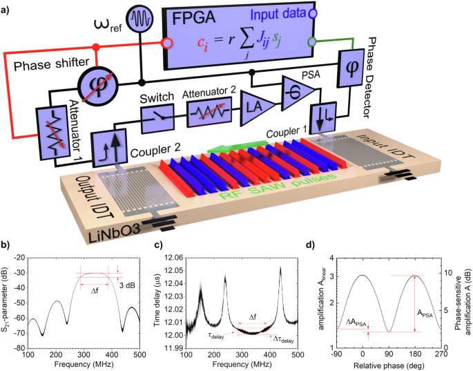
a SAWIM schematic: LiNbO₃ is a substrate of the SAW delay line. Coupler 1 is used to deflect −15 dB of the propagating RF pulses to a Phase Detector. PSA is a parametric phase-sensitive amplifier. LA is a microwave linear amplifier. Attenuator 2 is used to control the overamplification in the loop. The switch forms 58 RF propagating pulses within 12 μs round trip time in the loop and has a control square signal with a frequency of 4.829 MHz and a 50% duty cycle. ω_ref is a reference signal of 320.118 MHz that is used by PSA, phase detector, and phase shifter. FPGA is a digital measurement and feedback block that performs matrix multiplication between the vector of spin values s_j and coupling matrix J_ij and controls coupling pulses with the c_i vector. The phase shifter has two states 0° and 180° and controls the phase shift of the coupling pulses according to the sign of the c_i vector. Attenuator 1 controls the amplitude of the coupling pulses according to the magnitude of the c_i vector. Coupler 2 injects the coupling pulses into the propagating RF pulses with −15 dB of attenuation. Output and input interdigital transducers (IDTs) are used to excite and receive propagating surface acoustic waves. b Measurement of S₂₁ of the LiNbO₃ delay line. Δf = 100 MHz is the acoustic wave spectral bandwidth measured at −3 dB. c The frequency-dependent delay time of the SAW delay line. τ_delay = 12 μs is the average delay time over Δf with a total deviation of Δτ_delay = 45 ns. d Amplification of the parametric phase-sensitive amplifier as a function of the relative phase between the propagating RF pulses and the reference signal ω_ref = 320.118 GHz, with a phase sensitivity of A_PSA =  6.1 dB.

Full size image

The first step in designing a SAWIM is to ensure the stable formation of circulating RF SAW microwave pulses in the multi-physics ring circuit consisting of the delay line and the peripheral electronics. The SAW delay line has 30 dB of attenuation, which is easily compensated for by linear and phase-sensitive amplifiers. According to the Barkhausen stability criterion, the total phase accumulation in the ring circuit must be an integer multiple of 2π, which is ensured by a proper choice of the reference frequency ω_ref (see Supplementary Note 1 and Supplementary Fig. S1 for the circuit design and the Barkhausen criterion). To realize bi-stable Ising spins, the propagating SAW pulses are phase-binarized using a phase-sensitive amplifier (PSA) (see Supplementary Note 2 and Supplementary Fig. S2 for the implementation of the PSA^{39,40,41,42,43,44,45}). It is important to note that microwave PSAs, similar to optical PSA, can have multiple peaks in their phase-sensitive characteristic, allowing the implementation of spin system simulators beyond the Ising model such as hyperspin machines^46,47. Additionally, phase-sensitive amplification can potentially be implemented directly in the delay line using traveling wave excitation sources^48,49,50, which could further miniaturize the system.

Once stable circulating SAW pulses have been established, they have to be interconnected to realize an Ising machine with a particular Ising Hamiltonian. We have designed a measurement and feedback block (MFB) based on a field-programmable gate array (FPGA) similar to the one used in a 100-spin CIM²². The system includes a −15 dB coupler (Coupler 1) to siphon off a −15 dB portion of the circulating signal, which is then fed to an RF/IF Gain and Phase Detector AD8302, an 8-bit analog-to-digital converter (ADC) AD9280, a Xilinx Spartan-6 XC6SLX9 FPGA with a matrix multiplication block, a phase shifter block, and an attenuator HMC472 (Attenuator 1). Finally, another −15-dB coupler (Coupler 2) injects the feedback coupling pulses (c_i) back into the main ring. An FPGA and ADC are clocked with a signal having the same frequency of 4.829 MHz but with a phase shift of 90° as compared to the control signal for the RF switch. This ensures that the phase of the propagating RF pulses is measured at their centers. Currently, we binarize the phase detector signal s_i to +1 and −1 values. However, we note that since the ADC has 8 bits of resolution, the phase signal can be processed with finer resolution.

The energy of an arbitrarily coupled array of N phase-binarized SAW pulses is proportional to the corresponding Ising Hamiltonian⁵¹,

where s_i = ±1 corresponds to in-phase/out-of-phase states of the phase-binarized pulses, J_ij is an arbitrary interconnection/coupling matrix, and h_i is an individual local bias field. J_ij controls the coupling between spin s_i and s_j by adding a coupling pulse proportional to the saturated amplitude and phase of s_i to a propagating pulse s_j. The same spin configuration s_i represents the maximum number of cuts in a MAX-CUT problem:

A specific MAX-CUT problem can be mapped onto the SAWIM by adjusting the pairwise coupling terms J_ij. The MFB calculates the necessary amplitudes and phases for the feedback coupling pulses (c_i) proportional to J_ij, an adjustment coefficient r, and the instantaneous spin state via:

The matrix multiplication ({sum }_{j=1}^{N},{J}_{ij}{s}_{j}) gets done within one cycle of the FPGA clock. Additional delays in the ADC, the digital attenuator, and the phase shifters introduce an additional four cycles of delay. In total, it takes five cycles of digital clock or five pulse repetition cycles, which fits into the propagation time of eight unused spins.

In contrast to CIMs which use pulsed coupling signal, we inject a constant signal with modulated phase and amplitude according to c_i values into the circulating RF pulses picked up with an output SAW IDT. Then, the combined signal gets modulated with an on/off RF switch into RF pulses. This removes any concern about the timing of the injection of the coupling signal. Note, that both digital attenuators are clocked with the signal of 4.829 MHz frequency and −90°s of the phase shift as compared to the control signal for the RF switch, which ensures that the change in attenuation happens when the RF switch is closed.

In our experiments, the coupling matrices J_ij have unitary coefficients. However, since the SAWIM is based on time-multiplexed oscillators with feedback, the value of the total coupling pulse combined from all the interconnected pulses to a single pulse should not exceed 20–30% of the saturated amplitude of the circulating pulses as it would lead to over-coupling between RF SAW pulses and potentially chaotization of the oscillatory circuit. To ensure optimum amplitudes of the coupling pulses, an adjustment coefficient r is introduced. On the other hand, when the total coupling pulse is less than 2–3% and has a negative phase, the necessary switching of the pulse will not happen due to over-amplification of the circulating pulses in the ring circuit. These limitations can be avoided when solving MAX-CUT problems by keeping the smallest amplitude of the coupling pulses above the switching threshold of 2% and limiting the maximum amplitude below a top threshold of 30%. We note that for more complex problems, such as the Traveling Salesman Problem⁵² and the Channel Assignment Problem⁵³, where the couplings between Ising spins should have a higher resolution, special mapping protocols might need to be established.

Thermal stability

We emphasize that implementing a time-multiplexed Ising machine with circulating SAW microwave pulses leads to a principally different level of thermal stability that is 4–5 orders of magnitude higher than in CIMs and 1–2 orders of magnitude higher than in the analogous SWIM. This dramatic improvement is explained by a confluence of several factors. The central carrier frequency in CIMs is in the 200 THz frequency range while the SAWIM carrier frequency is just 300 MHz. Second, despite the vastly different carrier frequencies, the round trip in the CIM and the SAWIM is almost the same: 24.7 μs and 12 μs, respectively. It leads to a vast phase accumulation in the CIM on the order of 10¹² degrees. In comparison, the SAWIM phase accumulation is six orders of magnitude smaller. This directly impacts the thermal stability via the temperature coefficient of delay (TCD) which translates to the resulting phase accumulation coefficient P_acc,TCD. Phase accumulation coefficient accounts for 1.7274 × 10^7 ∘C⁻¹ for CIMs but only 102.492 ^∘C⁻¹ for SAWIM, i.e., the values for CIM and SAWIM differ by 1.6854 × 10⁵ times which explains the superior thermal stability of SAWIM. (see Supplementary Note 3 and Supplementary Fig. S3 for details). Consequently, while the 100,000-spin CIM requires both a precise thermostat system with  ± 0.01^∘C accuracy and a phase-locked loop (PLL), the SAWIM can operate at room temperature without any temperature control and phase-locking systems. Moreover, SAWIM demonstrates a high signal-to-noise ratio (SNR) of the circulating RF pulses allowing mapping of combinatorial problems with finer resolution of the coupling coefficients (see Supplementary Note 4 for details on the SAWIM SNR).

We note that despite a similar design and smaller total phase accumulation of SWIM, the thermal stability of SAWIM is still 28 times better due to a large temperature coefficient of the delay time in YIG, 9729 ppm ^∘C⁻¹, which is 133 times higher than in the SAW delay line.

Moreover, due to the difference in carrier frequencies, SAWIM demonstrates a much better efficiency in terms of carrier periods per spin and spin duty cycle. While it is sufficient to have a few periods of oscillation for a wave package pulse to define an Ising spin, the first CIM spins had about 1 × 10⁶ periods, and the latest 100,000-spin CIM, with 30 ps light pulses, has about 6000 periods, while the pulse repetition period even in the latest CIM is limited to 200 ps mainly due to an FPGA bottleneck. Thus, the duty cycle in the latest CIM is 15%, while in SAWIM it can be increased up to 50%.

Finally, the total power consumption of the demonstrated SAWIM active blocks adds up to just 1.82 W and can potentially be further reduced to less than 0.5 W (see Supplementary Note 5 for details on the SAWIM power consumption). Its thermal stability, low power consumption, and benchtop design make SAWIM a commercially feasible contender for combinatorial solvers.

Computational performance

We demonstrate the principle of operation of our Ising machine and the main dynamical properties with MAX-CUT Ising problems with J_ij = −1, 0 and no Zeeman term, h_i = 0. We note that a Zeeman term can be successfully implemented with an additional injected signal, similar to CIM and SWIM^31,54. In Fig. 2a, b we show two random graphs, A and B, for two MAX-CUT problems with the corresponding chessboard representation of the J_ij matrices, where the black pixels correspond to J_ij = −1. Matrix A has N = 50 vertices, ∣E∣ = 301 edges, and a density of d = 0.2457, whereas matrix B has 50 vertices, 262 edges, and a density of 0.2139. The time traces for the phase detector signal and the microwave pulse amplitude are taken from the phase detector and are shown in Fig. 2c, e for matrix A, and in Fig. 2d, f for matrix B. In Fig. 2c–f, s we introduce a break in the scale and zoom in on single RF pulses to visualize the carrier signal and show that there are approximately 30 periods of carrier frequency per pulse. The time traces in Fig. 2e, f are colored according to the amplitude of the phase detector signal. As can be seen, the RF pulses in Fig. 2e, f have similar shapes, and both have uniform phases, thus making them the ideal equivalent of an Ising spin.

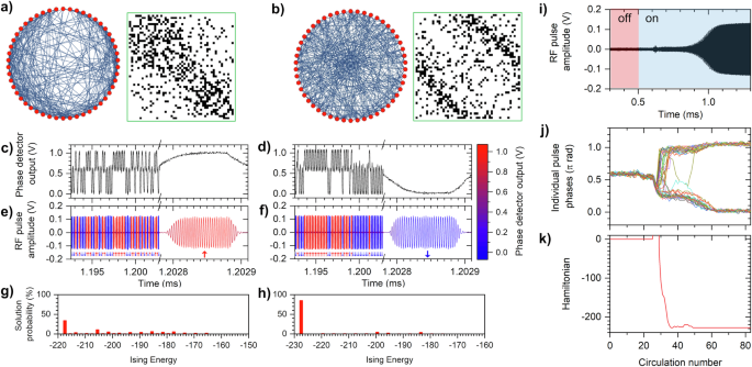
a, b Graph and chessboard representation of the solved MAX-CUT problems a Graph A and b Graph B. Red circles represent nodes. Dark blue lines represent edges. c, d Time traces of the phase detector output for Graph A and Graph B. e, f Time traces of the signal of RF pulse amplitude obtained from coupler 1. The time traces are colored according to the amplitude of the phase detector signal. The inset arrows demonstrate the corresponding up/down orientation of each quasi-spin. The data in (a–f) corresponds to an optimum solution of the MAX-CUT problems. g, h The solution probabilities as a function of Ising Energy. i Time traces of the SAW pulse amplitudes at the beginning of the computation process. During the first 200 μs from 0.3 till 0.5 ms, the overall loop gain is below −20 dB and there are only thermal fluctuations. At 0.5 ms the additional attenuation is switched off, and the system becomes active as the overall amplification in the small signal regime becomes 2 dB. j Temporal evolution of the individual discrete phase values of all 50 spins. k Temporal evolution of the Ising Energy of the Hamiltonian. The data in (i–k) corresponds to the random matrix B.

Full size image

For consecutive computations, we turn the amplification in the SAWIM loop on and off (see Fig. 2i) by an additional digital attenuator (attenuator 2) and control the supply of the linear amplifier with a square signal having a 10-ms period and a 95% duty cycle to ensure that between computation cycles the SAW echo pulses completely decay (see Fig. 2i, j).

We can see from Fig. 2j that most changes in the spin states happen already when the amplitude of the pulses is relatively small and the SNR is low so the effective temperature of the system can be considered high. Since the amplitude of the coupling pulses depends only on the spin configuration when the circulating spins have small amplitudes, the effective coupling is strong. Consequently, as the amplitude of the circulating pulses gradually increases, the effective coupling decreases, at the same time, the SNR increases and the equivalent temperature of the system decreases, and hence, the spin state freezes in local or global minima. Thus, the initial growth of the amplitude due to the amplification provides a natural annealing schedule, which can be tuned by e.g., compression gain of the amplifier. We note that controlling the SNR in the system may allow for ultrafast statistical sampling which is of interest for machine learning tasks with analog time-multiplexed Ising machines⁵⁵. In our implementation, switching the system on and off multiple times allows for the search for the global minimum of Ising Energy. This simple annealing method was chosen for the mere task of minimizing the Ising energy in our proof-of-principle SAWIM demonstration. In principle, more complex methods and systems suggested for CIMs can also be applied to improve the probability of finding a global minimum. For example, error-correction algorithms and chaotic amplitude control^56,57.

Finally, Fig. 2k shows the corresponding temporal evolution of the Hamiltonian. The solution probabilities for matrices A and B are shown in Fig. 2g, h. In both cases, the state with the highest probability corresponds to the optimum Hamiltonian, 34% of H = –218 for matrix A and 85% of H = –228 for matrix B.

Here, for demonstration, the single run time T_single-run is 10 ms, chosen simply because of the limitations of our basic data transfer protocol of the FPGA data acquisition system that we use for statistical benchmarking. This can be greatly improved with modern FPGA design techniques as done in CIM. In principle, the single run time can be reduced to 624 μs without reducing the success probability. First, it takes only two round-trip circulation periods to fully damp any high-order transit echoes in the SAW delay line, and therefore, the reset time can be reduced from 200 μs to 24 μs. Second, it takes 600 μs for the system to reach a near-saturation amplitude at which the effective temperature is significantly reduced and the spin state freezes (see Fig. 2j). Nevertheless, for consistency of the results, we calculate the system parameters for a value of 10 ms for a single run and only mention the possibility of reducing it down to 624 μs. Thus, taking into account the SAWIM computational schedule and power consumption of 1.82 W, the required energy to obtain a single solution for a 50-spin MAX-CUT problem is 18.2 mJ.

To compare our system with the 100-spin CIM, we characterize the probability of finding a ground state for Möbius ladder graphs of different sizes (8–50). We use 5000 system runs of 10 ms each to accumulate the statistics. Similarly to the CIM, the ground state probability starts to decay from 100% at a graph size of 12. The distributions of the solutions by the Hamiltonian states for 8-spin, 16-spin, 32-spin, and 50-spin MAX-CUT problems are shown in Fig. 3b–e. Compared to the 100-spin CIM, the ground state probabilities for graph sizes from 28 to 50 are slightly higher, which we attribute to better phase stability in the system, as well as differences in the strength of the coupling between artificial Ising spins.

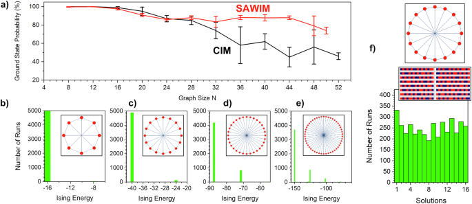
a Ground state probability and its standard deviations for Möbius ladder graphs of size N were obtained from 5000 consecutive runs of SAWIM and the corresponding data for 100-spin CIM extracted from Fig.3 of ref. ²² was obtained with 100 runs for each point. Error bars show standard deviation. b–e Distributions of the solutions by Ising energy of the system Hamiltonian for 8-spin (b), 16-spin (c), 32-spin (d), and 50-spin (e) Möbius ladder graphs. The insets show the corresponding graph configuration. Red circles represent nodes. Dark blue lines represent edges. f Distribution of the solutions by the states with the Ising Energy of −40 for a 16-spin (c) Möbius ladder graph. The inset shows the corresponding graph configuration and all 16 possible spin states.

Full size image

An important property of the Ising machine is the identity of the artificial spins, their coupling strengths, and the absence of any preferred direction for any spin, potentially arising from parasitic global or local Zeeman terms. To confirm that the SAWIM has no such bias, we performed 5000 runs with a 16-spin Möbius ladder graph coupling scheme. Due to the symmetry of the Möbius ladder graph, there are 16 states with the same ground state energy –40 (see the insets of Fig. 3c, f). It can be seen from Fig. 3f that the distribution of all the solutions by 16 possible states is mostly uniform. It confirms that the SAW Triple Transit Echo (TTE) level is low, and that there are no unintended couplings between the nearby circulating SAW pulses. Additional experiments confirming the absence of any preferred direction for any spin using the system runs with zero coupling matrix can be found in Supplementary Note 6 (see Supplementary Fig. S4).

To comprehensively benchmark our system with a standard set of MAX-CUT problems, we have chosen BiqMac lib. We generated 10 random J_ij matrices for each interconnection density from 0.1 to 0.9 with a step of 0.05. The matrices were generated by issuing the command rudy -rnd_graph n d s using Rinaldi’s graph generator rudy, where n = 50 is the number of vertices, d ∈ {0.10, 0.15, . . . , 0.90} represents the density, and s is a random seed that varied from 1000 to 1009 for each of the densities. In total, we benchmarked SAWIM with 170 different MAX-CUT problems. To gather statistics, we used 500 runs for each MAX-CUT problem with a corresponding J_ij matrix. To find the global minimum of Ising energy for each matrix, we used the standard Monte Carlo method implemented in the Matematica software with 20,000 runs. There were only two matrices out of 170 whose minimum Ising energy found by SAWIM differed from the global minimum. Most importantly, the difference between the found local and global minima is only 2%. Figure 4 shows an average success probability as a function of density. Since for many combinatorial problems approximate solutions can also be accepted and a more important parameter is the success probability and the time-to-solution parameter, we also present in Fig. 4 the success probabilities of obtaining a solution that is within χ% of the optimal (maximum cut) solution. As expected for such size of the combinatorial problem, the success probability for an exact solution varies between 1.2% and 9%. In comparison, for the 100-spin CIM, the success probability for an exact solution is below 6% for densities between 0.1 and 1. However, similar to CIM, for a SAWIM 99%-accurate solution, the success probability increases sufficiently. We note that in SAWIM, the success probability for the approximate solution grows and reaches its maximum at the density of 0.9, while in 100-spin CIM, there is a significant drop in success probability at this density for all values of approximate accuracy.

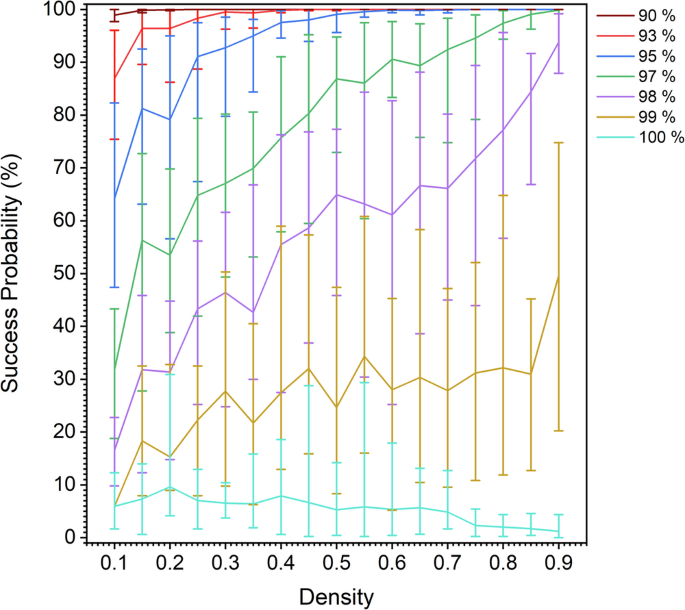
Success probability of obtaining a solution that is within χ% of the optimal (maximum cut) solution where χ is (90,93,95,97,98,99,100)% shown as the lines with the corresponding color (brown, red, blue, green, purple, yellowish-brown, and cyan). Error bars show standard deviation. We note that 100% corresponds to an exact solution, while 9{x}% corresponds to an accumulated number of solutions with relative values from 9{x}% to 100%.

Full size image

Optimal coupling

As suggested in ref. ⁵⁸, there exists an optimum coupling strength for oscillator-based IMs: if the coupling is too weak, the system does not reach a stable solution; if the coupling is too strong, non-optimal, local minima might hinder the IM from reaching its ground state. Since the SAWIM is constructed with electronic microwave amplifiers, which are intrinsically nonlinear, there is an optimum level of coupling between spins when the probability of the optimum solution is maximal. To verify the applicability of this theoretical prediction to time-multiplexed Ising machines, and particularly to our SAWIM, we introduced a numerical toy model, where each time-multiplexed Ising spin can be considered as a separate weakly nonlinear oscillator with a delay in a feedback loop. The evolution of the complex amplitude a_j of the jth spin, can be described by the following equation⁵⁹, which has been demonstrated to be applicable to time-multiplexed IMs³⁰:

where δp_j,τ = (p_j(t − τ) − p_s)/p_s, τ = τ_delay is a delay time along the loop, Γ₀ describes losses, ω₀ is the resonance frequency, K the gain, β_r the positive coefficient of the gain compression, β_i the nonlinear frequency shift, and p(t) = ∣a(t)∣² the power of oscillations with an operating point at p_s. The right-hand side of Eq. (5), (xi (t)={K}_{e}{exp }^{i{omega }_{e}t}{a}_{j}^{* }+kappa {sum}_{i}{J}_{ij}{a}_{i}/| {a}_{i}|), contains signals from the outer loops, i.e., the synchronization signal at the double frequency ω_e ≃ 2ω₀ and couplings from other spins, where κ is a coupling coefficient. For the simplicity of calculations, we chose the following parameters: ω₀/2π = 1.0, ω_e/2π = 2.002, τ = 10.0, Γ₀/2π = 4.0 × 10⁻², β_r = 2 × 10⁻², β_i = 1.0 × 10⁻⁴, K/2π = 4.0 × 10⁻², K_e/2π = 6.0 × 10⁻³.

The results of the calculations are shown in Fig. 5a. As expected, low values of the coupling strength make the probability of reaching the ground state negligibly small, whereas for strong coupling the IM exhibits an elevated risk of getting stuck in local minima, which also reduces the probability of finding the optimal solution. Thus, our calculations emphasize the need to find optimal coupling strengths, in agreement with ref. ⁵⁸.

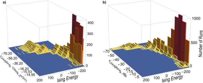
Distribution of the solutions at the states with different Ising energy: a for the numerical model, b produced by the hardware SAWIM. The additional attenuation of coupling strength is indicated with the labels on the left side. The inset in the middle shows the graph and chessboard representation of J_ij coefficients of the matrix B. The results are presented for 1000 runs per coupling attenuation.

Full size image

To corroborate these results with experiments, we performed a series of SAWIM runs with different global attenuation of the coupling strengths. Fig. 5b. shows how the distribution of the Ising energy of the solutions of the MAX-CUT problem defined by matrix B changes with coupling strength. The top distribution corresponds to zero coupling, resulting in random spin configurations with a wide Gaussian distribution of the Ising energies. As the coupling strength increases, the distribution width narrows sharply, and the mean rapidly moves to lower energies. At −11 dB of attenuation, 100% of the solutions are optimal at −228. However, when the coupling strength is attenuated by 5 dB, the distribution of the solutions again spreads to higher Ising energies, but now with a more scattered, non-Gaussian, distribution, reflecting how the system gets stuck in a few local minima. We note that 100% probability for an optimal solution can only be obtained for a limited number of random matrices and that a particular matrix B is chosen for demonstration purposes only.

We then benchmarked the success probability as a function of coupling strength with a set of 10 MAX-CUT random optimization problems with density 0.5 generated with Biq Mac lib that we used for our general benchmarking. Fig. 6a shows an averaged success probability of obtaining a solution that is within χ% of the maximum number of cuts for the benchmarking matrices. In the case of a 99%-accurate solution, the success probability reaches 83.3% and the corresponding time-to-solution parameter improves from 597 ms to 25 ms. A 99%-accurate time-to-solution (TTS) parameter is defined as TTS₉₉ = T_single-runln(1 − 0.99)/ln(1 − T_single-run) where T_single-run is 10 ms. Figure 6b, c shows the maximum and the minimum success probability for all the matrices. In order to visualize the evolution of the success probability we show separately in Fig. 6d–f success probability for 99%-, 98%- and 95%-accurate solutions for each benchmarking MAX-CUT problem. As can be seen from Fig. 6d there are matrices for which 99%-accurate solutions can be achieved. We note that an optimum level of relative attenuation is individual for every matrix. The details on the solution distribution for different attenuation levels for each benchmarking matrix can be found in Supplementary Note 7 (see Supplementary Fig. S5–S14).

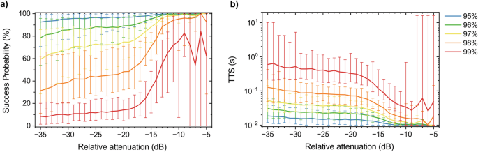
a Success probabilities and b TTS, time-to-solution parameters as a function of relative attenuation for solution qualities (95, 96, 97, 98, 99)% shown as the lines with the corresponding color (blue, green, yellow, orange, and red). Error bars show standard deviation and indicate variability for matrices of different seed numbers. The results are obtained with ten random Biq Mac matrices. We note that for a solution of a certain quality 9{x}%, we take all the solutions whose MAX-CUT values are above 9{x}% of the global maximum, i.e., 9{x}% till 100%.

Full size image

Thus, our experiments confirm that the time-multiplexed SAWIM has an optimum global coupling strength at which the stability of the ground state is maximized, reaching a 100% success probability. Although this level is individual for every matrix, on average at a relative attenuation level of −6 dB the success probability of obtaining 99%-accurate solution for MAX-CUT problems reaches 84%.

Scalability

We demonstrated our 50-spin SAWIM using a 50-mm long SAW delay line with a 12-μs delay, which could theoretically accommodate up to 200 spins. To further scale up the number of spins, one could explore various directions, such as increasing the delay time, increasing the central frequency (f), and reducing the SAW pulse width. As acoustic losses exhibit a f² dependence, lower central frequencies can result in 1 ms and even 10 ms delay time^60,61,62; operating at 100 MHz with a delay time of 1–10 ms could hence make the number of spins approach 10⁴–10⁵. On the other hand, low frequencies and long delay times lead to a corresponding increase in the time-to-solution, and, therefore, the use of SAW delay lines operating at the GHz range is of interest for high-speed solutions. SAWs can be excited and propagate efficiently with acceptable losses at frequencies up to 4–6 GHz^63,64, which would allow for 2–3 ns SAW pulses, and with μs-delay times could also reach thousands of equivalent Ising spins.

Once the maximum number of spins per delay line has been reached, one may explore the use of multiple delay lines, either in series or as parallel loops with individual linear and phase-sensitive amplifiers. In the case of series interconnection, the use of intermediate electronic or integrated SAW PSAs^48,49,50 would keep the SNR of the propagating SAW RF pulses similar to the present study, and the temperature stability would also remain the same, as the intermediate PSAs correct the phase of the circulating RF pulses. The advantage of series interconnection is the possibility of using a single MFB system. In this case, the time-to-solution parameter will rise in proportion to the circulation time. In contrast to the series interconnection scheme, the system of parallel loops would keep the time-to-solution mostly proportional to the circulation time of a single loop, at the cost of multiple MFBs. Using a combination of these approaches, the SAWIM hence has the potential for scalability up to 10⁴–10⁵ spins, while retaining its advantageous high-level temperature stability and high dynamic range.

In order to make our projections realistic and objective, we present an example design and SAWIM number of spins based on the delay line parameters reported in ref. ⁶¹. The referred SAW delay line has a central frequency of 85 MHz, 65 MHz of bandwidth, and 0.907 ms of delay time. Given the central frequency and the bandwidth, the suggested delay line can easily accommodate 15,419 RF pulses with five periods of central frequency corresponding to 15,419 equivalent Ising spins. The losses of 60 dB can be easily compensated with a cascade of modern microwave amplifiers that consume as little as a few mW^65,66. Connected in series, seven such delay lines will accommodate more than 100,000 equivalent spins. In this case, the temperature coefficient of phase accumulation ϕ_accum TCD for each delay line is only just 2.206° × 10³ °C⁻¹ which is still almost four orders of magnitude better than in CIMs.

Finally, in the current implementation, SAWIM starts from a random configuration and finds a local or global minimum that belongs to the same attraction basin. We note that since SAWIM has the same architecture as the latest CIMs and, therefore, can operate under the minimum gain principle²³ optimizing the search algorithm and potentially improving the time-to-solution parameter. The amplification in the loop can be gradually increased with voltage-controlled analog or digital attenuators giving enough time for the system to start up at the lowest energy state corresponding to the Ising Hamiltonian’s minimum state.

Performance comparison with other Ising machines

In order to evaluate the SAWIM position within a wide class of physical Ising machines, we benchmarked our SAWIM with other state-of-the-art implementations of Ising machines (Fig. 7). We have picked relevant metrics that affect the throughput of the system (connectivity, time-to-solution), system energy efficiency (system power consumption and energy required to reach solution) and energy efficiency per spin, system stability (the requirement of cryogenic systems and thermostats, coherence times for spins), system size and potential for scalability (connectivity, scalability of the success probability and projected number of spins). For a wide-scale comparison, we included in the benchmarking the state-of-the-art commercially available solution D-Wave 2000Q quantum annealer, containing 2048 qubits^13,67, and a noisy mean-field annealing algorithm running on an NVIDIA GeForce GTX 1080 Ti GPU⁶⁸. To highlight solutions based on different physical principles but having a high potential for CMOS integration, we considered a discrete-time memristor-based hybrid analog-digital accelerator implementing a Hopfield neural network (mem-HNN)¹² and an Ising Hamiltonian solver based on coupled stochastic phase-transition nano-oscillators¹⁴. The last four IMs are from the same class of time-multiplexed Ising machines: a 2000-node Coherent Ising Machine²¹, a state-of-the-art 100,000 spin Coherent Ising Machine²⁰, an alternative simplified optoelectronic CIM²⁹, a large-scale multi-wavelength optoelectronic CIM²⁸ and, finally, SAWIM. The SAWIM has a comparable or even better time-to-solution parameter relative to the first four candidates with the potential of a sufficient increase in the number of spins inherent for time-multiplexed systems.

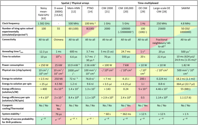
Note that favorable, average, and less advantageous values are highlighted in green, yellow, and red, respectively. ^aOscillation frequency of phase-transition oscillators. ^bProjected number of artificial spins according to the potential in scalability and taking into account mainly technical limitations in the physical carrier system ^cIn ref. ^{70 d}Several delay lines with different delay bits allow mapping onto optoelectronic CIM only a limited number of MAX-CUT problems but an all-to-all interconnection scheme with an FPGA system is also possible similar to 100,000-spin CIM, OE-CIM, and SAWIM. ^eMostly limited by the data acquisition interface and potentially can be reduced by 3–5 orders of magnitude. ^fFive hundred microseconds is the time to reach saturation in propagating SAW RF pulses. Since the amplitude of the coupling pulses only depends on J_ij and the phases of the propagating SAW RF pulses s_i, the settling time of 500 μs is identical to the annealing time. ^gThirty microseconds is simulation while in the experiment only 3.795 ms was achieved. ^hPower consumption and energy efficiency were simulated. ⁱPower consumption and energy efficiency were calculated for simulated PTNO IM with 100 spins without taking into account the power consumption of the control PC. ^jCoherence times for the spins in the steady state ^k,l Despite e^−N scaling of success probability for small problems, the interconnection issues at a large number of equivalents Ising spins may require the use of Chimera or sparse interconnection schemes that affect the scaling of success probability. ^oTen milliseconds corresponds to a single SAWIM run while 24.9 ms refers to TTS_99% time-to-solution for 99%-accurate solution for a random matrix under optimal coupling. The numbers in breaks are the corresponding values calculated for the time that takes to reset and obtain the solution without pauses for data acquisition in an FPGA.

Full size image

The absence of physical delay systems in seemingly simplified optoelectronic CIMs²⁹ in fact requires a more complex FPGA control system²⁹ than in classical CIMs^20,21 which has to store the amplitude and phase of the spins with high precision that significantly limits the maximum number of Ising spins. In the case of large-scale optoelectronic CIM²⁸, the absence of a physical delay system is compensated by the use of constant delay-time delay lines that dramatically limit the variety of possible encoded problems, essentially limiting the large-scale optoelectronic CIM to laboratory demonstrations without the possibility of solving arbitrary problems.

As compared with classical CIMs^20,21, the use of a solid-state SAW delay line operating at a central frequency of 320 MHz results in high thermal stability that is by a factor of 1.6854 × 10⁵ better than in CIMs^20,21. In contrast to the 100,000-spin CIM²⁰ and the large-scale optoelectronic CIM²⁸, this allowed for operation without a PLL. However, for even higher stability in larger and commercial SAWIM systems, we anticipate using simple PLL circuits.

Our SAWIM demonstrator has a power consumption of just 1.82 W and an energy efficiency of 55 solutions per second per watt, which is comparable with the 2000-spin CIM²¹ and several orders of magnitude better than D-Wave’s quantum annealer, while still having all-to-all connectivity and scalability potential. To consider the difference in the number of supported equivalent Ising spins, we introduce in our benchmarking two additional metrics—energy-to-solution per spin, and energy efficiency per spin. Regarding energy efficiency per spin, the current proof-of-concept SAWIM is still considerably less efficient than large-scale CIMs due to its small number of spins. However, we believe that if up-scaled, the SAWIM energy efficiency per spin can surpass that of CIM due to the possibility of reducing the single run time by orders of magnitude with the use of higher central frequency, faster repetition rate, and, most importantly, increased thermal stability that allows operating without a power-hungry thermostat system. However, due to the O(N²) scaling of the power consumption for the FPGA-based matrix multiplication scheme, the FPGA power consumption will be the major contribution for large-scale time-multiplexed Ising machines with the number of spins above 10⁴−10⁵.

Finally, SAWIM is smaller than most systems and has a good prospect for further system miniaturization due to the compatibility of SAW technology with standard CMOS fabrication⁶⁹.

We have demonstrated the design of a time-multiplexed surface acoustic wave Ising machine. The SAWIM has a circulation time of 12 μs and a time-to-solution parameter of 10 ms with the prospect of further reduction to 624 μs for 50-spin MAX-CUT problems, consuming only 18.2 mJ to compute a single solution. We have benchmarked our SAWIM using different size Möbius ladder graphs and random MAX-CUT problems of different densities from Biq Mac lib. We demonstrated that SAWIM has a comparable computational accuracy while having 4–5 orders of magnitude better thermal stability than CIMs. We have also demonstrated the importance of an optimized coupling strength at which the probability of the 99%-accurate solution reaches 84%. The SAWIM consumes just 1.82 W of power and has significant potential for further power reduction. Our work presents a versatile, low-power, fast, and cheap microwave-based time-multiplexed Ising machine platform, with the potential for significant miniaturization and dramatic improvement of temperature stability as compared to CIMs. The high SNR and dynamic range of coupling strength will allow for the implementation of high-resolution coupling matrices, enabling the mapping of more complex problems, such as the traveling salesman problem, the nurse scheduling problem, and channel allocation problems. Finally, we presented a clear scalability pathway and a detailed example of increasing the number of spins over 100,000 while still having almost four orders of magnitude better thermal stability as compared to 100,000-spin CIM which promises a high potential for commercialization.

Sample

The lateral dimension of the SAW waveguide is 50 × 10 mm². The microwave-to-acoustic wave transducers are silver IDTs. The substrate is lithium niobate.

Electrical measurements

The group delay presented in Fig. 1c was obtained from phase-delay measurement of the S-parameters using a vector network analyzer. The S-parameters were measured across a wide range of frequencies starting from 100 MHz to 500 MHz with a resolution of 10 kHz and 40,000 points. The group delay is calculated as the negative derivative of the phase shift with respect to the frequency. This calculation was performed using a built-in function of a vector network analyzer Rohde & Schwarz ZNB 40. The time delay plot was smoothed with an FFT filter with 10-point integration.

The phase-sensitive amplification curve was extracted from the envelope of an amplified signal with constant amplitude and frequency detuned from the reference signal frequency by 10 MHz. The frequency detuning introduced a continuous phase drift with a period of 1 μs, which allowed a smooth phase-sensitive amplification curve to be extracted. The details on the design of the phase-sensitive amplifier can be found in Supplementary Note 2.