Self-reports map the landscape of task states derived from brain imaging
Introduction
Variation in psychological states plays a prominent role in the health, well-being, and productivity of members of society1. Descriptions of psychological states are made possible by the uniquely human capacity for introspection2. For almost a century, however, uncertainty regarding the accuracy of introspection has meant that relationships identified in this way are often treated with scepticism3,4. Recent work has successfully combined data derived from introspective reports with laboratory techniques that map objective features of behaviour, establishing that when collected appropriately, introspective data can contain meaningful information regarding underlying psychological processes (for reviews, see5,6,7,8,9:). In particular, correlational studies conducted over the last two decades using experience sampling have established relationships between self-reported descriptions of experience and objective indicators of cognition, such as task performance10, changes in behaviour in daily life11,12, and covert measures of cognition derived from state-of-the-art brain imaging that describes both brain function13,14,15 and structure16. These correlational studies establish that self-reported descriptions of experiential states could, in principle, be used as a tool to complement objective descriptions of human cognition.
Our study builds on this emerging evidence to assess the accuracy with which self-reports can describe different psychological states. We used experience sampling to build a description of the states that emerge as healthy participants perform a variety of different tasks that sample a range of different underlying cognitive processes. These include (1) the ability to maintain information within working memory15,17, (2) the ability to sustain attention18, (3) the ability to exert motor control17, (4) the ability to reflect on the self and on other people19, (5) the ability to retrieve autobiographical memories20, (6) the capacity for reading20, and (7) the ability to watch movies21. Note, however, that while our study maps a wide range of different situations, it is in no way an exhaustive list of the tasks that humans can perform.
While participants completed this battery of tasks in the behavioural laboratory, we collected descriptions of their ongoing thought patterns using multi-dimensional experience sampling (mDES). mDES asks participants to describe their experience by rating their thoughts along a number of dimensions on multiple occasions (for a review see9:). Prior studies have shown that mDES is sensitive to objective indicators of cognitive function measured in the laboratory (including functional magnetic resonance imaging (fMRI)14,15,22,23, EEG24, and measures of brain structure25,26) and distinguishes activities performed in the laboratory27 and in daily life11,12. In this study, we used a battery of 16 mDES questions which are presented in Supplementary Table 1. These same mDES questions have been previously used in studies examining experience during movie watching28 and in an analysis of the links between cognition in daily life and mental health29.
Variation in introspective descriptions of experience across tasks was then compared to variation in patterns of brain activity that these tasks engage (based on prior fMRI studies from large groups of other participants, for which unthresholded maps of the tasks compared to the implicit baseline were available). To do this, we used machine learning methods to build a generative model (referred here to as ‘state-space’) of the relationship between states defined via introspection and features of brain activity. Finally, we confirmed this model in a new sample of participants using four exemplar tasks from our initial task battery that characterized key features of our ‘state-space.’
Methods
Overview of analytic approach
To map introspective descriptions of states onto objective measures of brain activity, we used a ‘state-space’ approach similar to that used in our prior studies14,28,30,31. In line with these, we used two separate multi-dimensional spaces, a 5-d ‘thought-space,’ generated by applying Principal Components Analysis (PCA) to the mDES data (Fig. 1a), into which we then projected each original mDES observation, and, a 5-d ‘brain-space,’ generated using an existing decomposition32 of resting-state connectivity data from the Human Connectome Project (HCP)21 (Fig. 1b). We projected group-level unthresholded brain maps for each of the tasks used in our study onto these dimensions, yielding a set of coordinates that describe the similarities between the whole-brain states that each task engenders. Next, we used Canonical Correlational Analysis (CCA)33 to map these two multi-dimensional spaces together, forming a ‘state-space’ that combines introspective descriptions of ongoing thought patterns during tasks with patterns of brain activity recorded in the same tasks. Finally, we evaluated the generalizability of this model by collecting new experience sampling data for a subset of exemplar tasks based on their locations in the ‘state-space’ and examined how well introspective descriptions of experience in this unseen self-report data recapitulated the location of these tasks in the initial ‘brain-space’. The current study was not pre-registered.

We used two multi-dimensional spaces: a ‘thought-space’ generated by applying PCA to introspective reports collected using mDES (see top-right for example questions) while participants performed 14 different tasks in the lab (see Methods). PCA yielded 5 dimensions, displayed as word clouds (bottom-left) in which font size indicates the importance of an experiential feature, and colour indicates polarity (i.e., features with same colour load on component in same direction; red = positive, blue = negative). These PCA dimensions form the dimensions of the ‘thought-space’ and each original mDES observation (16 items) was projected into this 5-d space. 3-d scatter plot shows the task averages of these projected scores along the first three ‘thought-space’ dimensions. b ‘brain-space’ generated using an existing decomposition32 of resting-state connectivity data from the HCP21 into which we projected 14 whole-brain, group-level unthresholded fMRI task maps, gained from different sets of individuals from prior fMRI studies. Whole-brain maps from a set of exemplar tasks used to subsequently test the generalisability of our combined ‘state-space’ in unseen data (see Methods) are shown in the top-right (Supplementary Fig. 5 presents all maps), while the dimensions derived from the HCP data are shown in the bottom-left (Supplementary Fig. 1 presents lateral and medial views). 3-d scatterplot shows the location of task maps along the first three ‘brain-space’ dimensions. Note: 3-d plot labels are jittered to prevent overlap of terms (see Supplementary Table 6 for exact task-average locations in ‘thought-space’ and Supplementary Table 3 for exact locations in ‘brain-space’).
Participants
Original sample: full 14-task battery
194 participants were recruited to complete the full 14-task battery in a behavioural laboratory. The sample size was guided by the sample sizes of prior studies in the literature that have investigated differences in ongoing thought across easy and hard task contexts22,27,34,35. This sample was drawn from the undergraduate student population at Queen’s University, Canada. The study was approved by the institutional ethics committee at the Queen’s University Psychology Department and followed all relevant ethical regulations. All volunteers provided informed written consent and received 2 course credits for their participation. Demographic information was missing for four participants due to errors in data collection. These four participants were excluded from all analyses, resulting in a final sample of 190 participants. Of these 190 participants, 164 identified as women, 24 as men, and two as non-binary or similar gender identity. Mean age of participants was 18.56 years (SD = 1.09, range = 17–24 years). All 190 participants contributed 38 mDES observations each, resulting in 7220 total observations.
Replication sample: subset of 4 tasks
101 participants were recruited to complete a subset of 4 tasks from the full 14-task battery. The sample size was guided by time and resource constraints, aiming for a minimum of 100 participants before the mid-term break. This sample was also drawn from the undergraduate student population at Queen’s University. The study was approved by the institutional ethics committee at the Queen’s University Psychology Department and followed all relevant ethical regulations. Demographic information was missing for five participants due to errors in data collection. These five participants were excluded from all analyses. In addition, one participant was removed from analyses as they were missing over half their data due to a technical error during data collection, leaving a final sample of 95 participants. Of the remaining 95 participants, 87 identified as women, 6 as men, and 2 as non-binary or similar gender identity. Mean age of participants was 18.24 years (SD = 1.05, range = 17–24 years). 94 out of 95 participants contributed 11 observations each, with one participant missing one observation due to a technical error in data collection, resulting in 1044 total observations.
Procedure
Full 14-Task Battery
Participants attended one 2-hour study session in the behavioural laboratory to complete the 14-task battery. Participants provided written informed consent before the study session began and provided their demographic information via a demographic questionnaire. Once consent and demographic information were acquired, participants completed the 14-task battery in a room alone with a computer. Participants were asked to refrain from using any technological devices (phones, smartwatches, tablets, laptops/computers) besides the computer in front of them to avoid distractions. The task battery was presented using PsychoPy336 and included the following 14 tasks, grouped into seven pairs based on task similarity: (1) Easy-/Hard-Math, (2) Finger-Tapping and Go/No-Go, (3) Self-/Friend-Reference, (4) 0-/1-Back, (5) 2-Back-Faces/-Scenes, (6) Autobiographical Memory and Reading, and (7) passive viewing of Documentary and Sci-Fi videos.
There were three task blocks per task, except for the passive-viewing (Documentary and Sci-Fi) and Two-Back (Faces and Scenes) tasks, which had two blocks each (38 task blocks total). Within each task, task blocks were randomized (except the passive-viewing tasks). Across tasks, each task block lasted ~90 s, jittered by ± 15 s. Task pairs were presented consecutively. Within task pairs, task order presentation was randomized, and the task pairs were randomized based on a unique seed generated for each participant. Written instructions were presented at the start of each task block. Immediately after each task block, participants were prompted with mDES questions about their thoughts during the previous block. The task battery took participants approximately 1.5–2 h to complete. Full code for the presentation of the 14-task battery is openly available on Zenodo: https://doi.org/10.5281/zenodo.14290073.
Shortened 4-Task Battery
The procedural details for the shortened task battery were identical to those of the full task battery, except only four tasks were presented in a randomized order across participants: (1) Hard-Math, (2) Go/No-Go, (3) Autobiographical Memory (4) Documentary. There were three task blocks per task, except for the passive-viewing Documentary task which had two blocks (11 task blocks total). The task battery took participants approximately 30–60 min to complete. Full code for the presentation of the 4-task battery is openly available on Zenodo: https://doi.org/10.5281/zenodo.14290092.
Multi-dimensional experience sampling (mDES)
Participants’ ongoing thought was measured using mDES. Each mDES probe was made up of sixteen items (see Supplementary Table 1), presented in a random order. All items were rated by participants on a continuous scale of one to ten, using the left and right arrow keys to move a marker on a screen (see Fig. 1a for examples). The marker start location was randomized for each item. When participants were satisfied with the marker position on the scale, they pressed ‘Enter’ to confirm their answer and move on to the next item. mDES probes were presented at the end of each task block. Overall, participants completed a total of 38 probes in the full 14-task battery and 11 probes in the shortened 4-task battery.
Self-/friend-reference task
This task pair was adapted from Murphy and colleagues19. Participants were required to make judgments as to whether a presented adjective applied to either to themselves (‘self-reference’) or a friend of choice (‘friend-reference’; note, in Murphy and colleagues’ study19, this condition referred to ‘another person’, rather than a ‘friend’). Participants were instructed to attend to the centre of the screen, where adjectives were presented one word at a time. Adjectives were either positive (e.g., ‘enthusiastic’) or negative (e.g., ‘insecure’). Participants had to indicate whether they would associate the word presented with the referent (self or friend) or not using the left and right arrow keys. For the ‘friend’ task, participants were instructed to think of a single friend throughout the task. Participants saw a unique list of words in each block which were counterbalanced across tasks.
Go/No-Go task
This task was adapted from Alam and colleagues18. Participants were required to either make a response (button press) or inhibit their response (no button press) depending on whether the stimulus presented was a ‘Go’ trial or a ‘No-Go’ trial. Each trial presented nonsense stimuli (scrambled word) framed in a rhombus outline for 0.75–1.25 s. Participants were instructed to focus on the slant of the stimulus’ outline. Outlines with a minor slant indicated a ‘Go’ trial, while boxes with a more significant slant indicated a ‘No-Go’ trial. In the current study, task blocks only included stimuli from the ‘hard’ condition from Alam et al.’s18 original study (slants more difficult to differentiate from each other). Participants viewed a fixation cross between trials for 0.5–1 s. Per Alam et al.18. each block contained 46–54 stimuli and consisted of 80% ‘Go’ trials and 20% ‘No-Go’ trials.
Finger-tapping task
This task was designed to mimic that of the Human Connectome project17 and adapted from a similar task used by Livesey and colleagues37. Participants were instructed to press the space bar when a black square was shown on the screen. A fixation cross appeared between square presentations. Squares were presented for 2 s, and failure to press the space bar on time was recorded as a failure. The delay between presentations was jittered, with a minimum delay being 2 s and a maximum delay being 5 s.
Passive viewing: documentary and Sci-Fi
Participants watched short clips from either the film ‘Inception’ (‘Sci-Fi’) or from the documentary ‘Welcome to Bridgeville’ (‘Documentary’). Presented clips were each 3 min and 46 s long, adapted from clips from the Human Connectome Project21. The volume of the clips was balanced to reduce large spikes in noise. Each movie presentation was interrupted at a random point after the first 15 s and before the last 15 s with an mDES prompt, with another shown at the conclusion of the clip (i.e., two MDES probes per video task).
2-back tasks: faces and scenes
This task was designed to mimic that of the Human Connectome project17. Participants indicated using a keypress whether a presented stimulus matched the one presented two trials before. In the 2-back ‘Faces’ task, presented stimuli were images of faces, while in the ‘Scenes’ task, presented stimuli were images of scenes (e.g., an outdoor garden or a living room). There were two task blocks for each 2-Back task. Each block comprised 35 trials with five instances of ‘target’ trials where a stimulus repeated two trials after its initial presentation and five instances of ‘target-lure’ trials where a stimulus repeated either 1 or 3 trials after its initial presentation. Each trial lasted 2 s, with an inter-stimulus interval of 500 ms.
Reading task
This task was adapted from Zhang and colleagues20. Participants read 15-word sentences presented one word at a time. After viewing a 1–3 s fixation cross, participants were presented with each of the 15 words 600 ms at a time.
Memory task
This task was adapted from Zhang and colleagues20. In each block, participants were asked to recall a memory upon viewing a cue-word (e.g., ‘Airport’) and to press ‘Enter’ when they had thought of one. They were then shown a fixation cross for 4–5 s. Following this, they were instructed as follows: “Now we would like you to think about this event. Please press Enter when you are ready to begin.” Participants were then shown a 20 s fixation cross, followed by mDES.
0-/1-back task
This task was adapted from Turnbull and colleagues15. Participants passively viewed non-target trials involving two different shapes (e.g., a square and a circle) presented for 0.5–1.5 s on either side of a vertical black line in the centre of the screen. After 2–8 non-target trials, a target trial occurred, where a smaller shape appeared over the line in the centre of the screen for 3.5–5 s (or until input was received) between either: a) two larger shapes in the 0-back condition, or b) two question marks in the 1-back condition. In the 0-back condition, participants indicated with a keypress whether the central shape matched the shape presented to its left or right side. In the 1-back condition, where question marks surrounded the central shape, participants indicated the central shape’s match from the previous non-target trial. A fixation cross was presented for 1–2.5 s between trials.
Easy-/hard-math task
This task was adapted from Wang and colleagues38. Participants viewed addition expressions and then indicated with a keypress which of two presented sums was correct. Each expression was presented for 1.45 s followed by two sums presented on the left and right sides of the screen for 1.45 s. In the ‘easy’ condition, expressions only involved one-digit numbers, while in the ‘hard’ condition, expressions included one two-digit number up to 19. Participants completed three blocks each of the easy and hard conditions involving 28 trials each. If the participant did not respond within 5 s, the task continued, and the response was counted as incorrect.
Task brain maps
The spatial maps summarizing brain activity in each of the 14 tasks were taken from a variety of prior fMRI studies, summarized in Supplementary Table 2. All task maps were (unthresholded) group-averaged z-stat contrast maps and contrasted the task condition against baseline. Therefore, each task map represents the group-averaged BOLD-signal in each task compared to baseline. Since the coverage of task maps differed, we created a binarized mask that removed any regions in which there were missing data in any of the task maps and applied this mask to all maps prior to the ‘brain-space’ analysis. All brain maps (including the gradient maps outlined below) used in the current study are openly available (https://doi.org/10.5281/zenodo.14112468).
Connectivity gradients: ‘brain-space’
The five connectivity gradients used in the current study were generated by Margulies et al.32, made openly available via Neurovault (cortical and subcortical): https://identifiers.org/neurovault.collection:1598. These gradients were generated by applying a non-linear dimension reduction technique (diffusion embedding) to the averaged functional connectivity matrix of the Human Connectome Project (HCP) resting state data21. These gradients explain whole-brain connectivity variance in descending order, such that the first gradient explains the most variance in the whole-brain connectivity data, the second explains the second most variance, and so on. Along each gradient, brain regions with similar connectivity profiles (to the rest of the brain) fall close together, and have similar ‘gradient values’, while regions with more distinct connectivity profiles fall further apart, and have more dissimilar ‘gradient values’39. This analysis, therefore, results in a spatial map for each gradient identified in which each parcel contains a ‘gradient value’. The first five gradients explain approximately 60% of the connectivity variance and prior studies have highlighted that the first three gradients relate to important features of cognition31,40,41. Supplementary Fig. 1a–e shows lateral and medial views of each of the brain maps representing each of the gradients and Supplementary Fig. 1f shows a radar plot representing the mean gradient values in each of the Yeo-7 networks42 for each gradient. We use these five gradients to construct the 5-d ‘brain-space’ (see Fig. 1b). These details are almost identical to those described in Mckeown et al.14.
Locating task states in ‘brain-space’
To locate the 14 task states in the 5-d ‘brain-space,’ we calculated the pairwise spatial correlations (Spearman rank) between each (masked) task brain map and each of the first five connectivity gradients described in Margulies et al.32. The code used for this process is openly available (https://doi.org/10.5281/zenodo.14112468). This analysis resulted in five correlation values for each task brain map, indicating where that brain map falls along each dimension. These correlation values act as ‘coordinates’ in the 5-d ‘brain-space’ (see Fig. 1b for a 3-d scatterplot showing the coordinates for each task state along the first three dimensions and Supplementary Table 3 for the five coordinates associated with each of the 14 tasks). To determine whether the associations between the task maps and gradient maps were above those associated with the artefactual features of the spatial maps (i.e., smoothing), we conducted a Spin test using the Neuromaps toolbox (https://github.com/netneurolab/neuromaps). See the openly available code associated with this study for further details.
Generation of ‘thought-space’
To construct the low-dimensional ‘thought-space,’ we applied PCA, with no rotation, to the mDES data from the full task battery sample (14 tasks; N = 190). PCA was applied at the probe-level in the same manner as our prior work (e.g.,11,14,27,35,43,44,45). Specifically, we concatenated the responses of each participant for each probe into a single 7220 × 16 matrix—in which each column was an experience sampling item (16 items), and each row was an mDES observation (7220 observations; 38 observations per participant). PCA was applied using the ‘ThoughtSpace’ package (https://doi.org/10.5281/zenodo.14112233), which uses scikit-learn46 for PCA computations.
To ensure that at least 50% of the total variance in the mDES data was explained by this low-dimensional ‘thought-space,’ we retained the first five components for further analysis (1st component = 21.28% explained variance; 2nd = 11.85%; 3rd = 9.16%; 4th = 6.61%; 5th = 5.89%; see Supplementary Fig. 2 for scree plot). This analysis resulted in a set of five PCA scores for each observation, indicating the prevalence of each PCA component identified for that observation (via the computation of the dot product between the component loadings of each component and the experience sampling items of that observation).
Generalizability of PCA ‘thought-space’
To establish the robustness and generalizability of the 5-d ‘thought-space,’ generated by applying PCA to mDES data from all 14 tasks, we performed a leave-one-out cross-validation analysis in which we systematically excluded mDES data associated with each task one at a time. For each iteration, we removed all mDES data related to a specific task from the original dataset (N observations = 570, apart from 2-back and passive-viewing tasks where N observations = 380), and applied PCA to the mDES data from the remaining 13 tasks. Next, we applied the trained PCA model to the held-out task data, resulting in observation-level PCA scores for the held-out task (via the computation of the dot product between the component loadings of each component from the held-out model and the experience sampling items of each observation in the held-out data).
Following the generation of observation-level PCA scores for each held-out task, we calculated the (two-tailed) Pearson correlation (and 95% CIs, Bonferroni-adjusted for 14 tasks) between the participant-averaged PCA scores for each task obtained from the omnibus PCA model—which was trained on all 14 tasks—and the participant-averaged projected scores derived from the held-out PCA model in which that task was held out (N = 190). We then made these correlation values and CIs absolute for plotting (see Fig. 2b).

a Word clouds representing the five thought patterns identified via PCA applied to mDES data from all 14 tasks in the task battery (each word = mDES item; the size of word = magnitude of item loading on that pattern; colour = direction of loading, red = positive, blue = negative). b Bar graphs showing the high correlations between PCA scores derived from the omnibus PCA (with all 14 tasks included) and the held-out PCA models (one task held out each time). Y-axis = which task was held out (and which task’s scores are being correlated), and X-axis = Pearson correlation value. Error bars = 95% CI, Bonferroni-adjusted for 14 tasks. c Bar graphs showing the predicted mean score of each thought pattern in each of the 14 tasks, derived from the LMMs comparing the held-out PCA scores between each task. Error bars = 95% CI, Bonferroni-adjusted for 14 tasks. d Word clouds summarizing the predicted mean of each thought pattern in each of the 14 tasks (each word = task; size = magnitude of the predicted mean PCA score; colour = direction, red = positive predicted value, blue = negative predicted value).
Generation of ‘state-space’
To assess whether there is a significant mapping between the two multi-dimensional spaces (‘thought-space’ and ‘brain-space’), we implemented CCA in Python [version 3.8.13] using the scikit-learn46,47 [version 1.2.1] package (N = 190, N observations = 7220). CCA is a multivariate technique that identifies the linear combinations between two sets of variables (X and Y) that maximizes their correlation. In our analysis, the X variables were the observation-level scores for each of the five PCA components (7220 × 5). The Y variables included brain coordinates at the task-level for each of the five gradients (14 × 5; see Supplementary Table 3). To align the dimensions, task-level brain coordinates were replicated for each occurrence of the corresponding task in the X variables (resulting in a matrix of size 7220 × 5). Both X and Y variables were z-scored before applying CCA.
We implemented permutation tests to evaluate the statistical significance of observed canonical correlations. To this end, the PCA rows were randomly shuffled 1000 times, and CCA was repeated on each shuffle to generate a ‘null’ set of canonical correlations on each iteration. The shuffle procedure involved first grouping PCA rows by participant ID, and then shuffling each participant’s rows using the current iteration number (0-999) as the seed, ensuring a consistent shuffle order across participants on each iteration. This procedure generated a null distribution of canonical correlations (see Fig. 3a). P-values were calculated as the proportion of permuted canonical correlations greater than or equal to the observed values. The alpha level was Bonferroni-adjusted to account for five dimensions (i.e., 0.05/5 = 0.01). A significant p-value indicates that identified associations between ‘brain-space’ and ‘thought-space’ are unlikely to have arisen by chance.
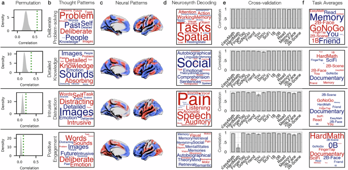
a Density plots showing null distribution of canonical correlations derived from shuffling PCA observations (N iterations = 1000). True canonical correlations represented as green dotted lines. b Word clouds representing how each CCA dimension organizes thought patterns identified via PCA applied to mDES data (each word = mDES item, size = magnitude of the summed weighted loading (see Methods), and colour = direction [red = positive, blue = negative]). c Spatial brain maps representing how each CCA dimension organizes whole-brain neural patterns identified by correlating task brain maps with dimensions of brain function variation (gradients; see Methods). In each map, positive values are red and negative values are blue. d Word clouds representing results from a Neurosynth meta-analysis identifying the most likely terms used to describe the pattern of brain activity seen in the CCA-weighted brain maps shown in panel C (size = magnitude of relationship, and colour = direction [red = positive, blue= negative)]). e Bar graphs showing consistency of CCA variates between omnibus CCA (all tasks included) and held-out CCA models (one task held out each time). Y-axis = which task held out and X-axis = Pearson correlation. Error bars = 95% CI, Bonferroni-adjusted for 14 tasks. f Word clouds summarizing the predicted mean score of each summed CCA variate in each of the 14 tasks (each word = task, size = magnitude of mean score, colour = direction [red = positive predicted mean, blue = negative predicted mean]).
Visualizing the CCA ‘state-space’
We next visualized the X variates (i.e., CCA-weighted PCA scores) using word clouds. For each X variate, we multiplied the (z-scored) PCA component loadings for each mDES item for each PCA component included in the CCA by the CCA’s X weight for that PCA component. This step resulted in, for each X variate, a new set of CCA-weighted component loadings for each PCA component. We then summed each mDES item’s CCA weighted loadings across all five components, resulting in one value for each mDES item for each X variate (see Fig. 3b). In each word cloud, a word is an mDES item, the size represents the magnitude of the summed weighted loading, and the colour represents the direction (red = positive, blue = negative).
Using spatial brain maps, we then visualized the Y variates (i.e., CCA-weighted gradient scores). For each Y variate, we multiplied the (z-scored) gradient values in each parcel for each gradient included in the CCA by the CCA’s Y weight for that gradient. This step resulted in, for each Y variate, a new set of CCA-weighted parcels for each gradient. We then summed each parcel’s CCA-weighted gradient values across all five gradients, resulting in one value for each parcel for each Y variate (see Fig. 3c). In each brain map, positive values are in red, and negative values are in blue.
Neurosynth decoding of CCA brain maps
Having created brain maps to visualize each Y variate, we used Neurosynth’s online meta-analytical decoder to identify cognitive and psychological terms most strongly associated with our maps in the available literature (four maps; one for each significant CCA dimension). The decoder identifies terms most strongly associated with the patterns of neural activity in each map by comparing the patterns of activity in the input map to patterns of activity in the brain maps available in the Neurosynth database. This results in a set of psychological, cognitive, and anatomical terms that are most likely to be associated with the patterns of activity in the input map14. To visualize the results of this analysis as word clouds, we selected the top ten positive and top ten negative cognitive and psychological terms associated with each map, retaining only the first term in instances of duplicates (e.g., ‘episodic’ and ‘episodic memory’) and excluding terms related to anatomy instead of function (e.g., ‘precuneus’)14. These word clouds are shown in Fig. 3d.
Generalizability of CCA ‘state-space’
To establish the generalizability of the CCA ‘state-space,’ we performed a leave-one-out cross-validation analysis in which we systematically excluded all X variables (z-scored PCA scores) and Y variables (z-scored brain coordinates) associated with each task one at a time (N observations = 570, apart from 2-back and passive-viewing tasks where N observations = 380). To prevent data leakage during the PCA process, we used the PCA models generated based on held-out data. Subsequently, we applied the trained CCA model to the held-out task data, resulting in observation-level CCA X and Y variates for the held-out task. To create one score for each set of X and Y variates, we summed the z-scored X and Y variates. We then calculated the Pearson correlation (two-tailed) between the participant-averaged summed CCA scores for each task obtained from the omnibus CCA model, which was trained on all 14 tasks, with the participant-averaged projected scores derived from the held-out CCA model (N = 190; 95% CIs Bonferroni-adjusted for 14 tasks). A consistently high correlation suggests a given CCA dimension is generalizable (i.e., is not unduly influenced by any single task).
Linear mixed models (LMMs)
LMMs were fitted by restricted maximum-likelihood estimation in R [version 4.1.148] using the lme4 package [version 1.1.3149]. We used the lmerTest package [version 3.1.350] to obtain (two-tailed) P values for the F-tests returned by the lme4 package. For each set of models, the alpha level for each F-statistic was set based on 0.05 divided by the number of models (i.e., Bonferroni-corrected alpha level). The reported p-values are unadjusted. Degrees of freedom were calculated using Satterthwaite approximation and for F-tests, type 3 sum of squares was used. Contrasts were set to ‘contr.sum,’ meaning that the intercept of each model corresponds to the grand mean of all conditions51. Estimated marginal means and their confidence intervals (shown in Fig. 2c and Fig. 3e) were calculated using the emmeans package [version 1.8.352] and Bonferroni-adjusted for the number of tasks (14). Across all models, to account for multiple observations per participant, ‘participant’ was included as a random intercept. In addition, across all models, age and gender were included as nuisance covariates. Finally, for all LMMS, we concatenated the PCA or CCA scores derived from the held-out models into one matrix. In cases where the held-out PCA or CCA component was flipped relative to the omnibus component (as indicated by a negative correlation between omnibus and held-out observation-level scores), we multiplied the observation-level scores by −1 for interpretability. Across all models, 190 participants were included (N observations = 7220; 38 observations per participant). Diagnostic plots confirmed normality and homogeneity of the residuals.
Task locations in PCA ‘thought-space’
To examine the differentiation of tasks within the PCA ‘thought-space,’ we performed a series of LMMs—one for each of the five thought patterns—to compare the observation-level PCA scores between each task context derived from the held-out models. Therefore, in each model, the outcome variable was the observation-level ‘PCA score’ and the explanatory variable was ‘task’ (14 levels).
Example model formula: lmer(PCA Component Score ~ Task + Age + Gender + (1|Participant)).
Task locations in CCA ‘state-space’
To examine the differentiation of tasks within the CCA ‘state-space,’ we performed a series of LMMs—one for each of the four significant CCA dimensions—to compare the observation-level summed CCA variates between each task context derived from the held-out models. Therefore, in each model, the outcome variable was the observation-level ‘CCA summed variate score’ and the explanatory variable was ‘task’ (14 levels).
Example model formula: lmer(CCA Dimension Summed Variate ~ Task + Age + Gender + (1|Participant)).
Prediction accuracy of brain states
To assess whether the CCA model, trained on all 14 tasks, can make accurate predictions of brain states using unseen experience sampling data, we collected new experience sampling data in an independent sample (N = 95) in a subset of 4 tasks (Memory, Go/No-Go, Documentary, and Hard-Math). These tasks were selected as they fall at the extreme ends of the first two CCA dimensions (see Supplementary Table 4 for task locations along all four significant dimensions). We projected the new experience sampling data from these 4 tasks into the omnibus PCA ‘thought-space’ trained on all 14 tasks in the original sample (via the computation of the dot product between the component loadings of each component identified in the original sample and the experience sampling items of each observation in the new data). We then used the trained CCA model to predict brain coordinates in ‘brain-space’ for each PCA observation (N observations = 1044) in the new sample using scikit-learn’s method ‘predict’46.
To assess the accuracy of these predictions, we first averaged the observation-level predictions by participant (resulting in each participant having one prediction per task so that these predictions can be compared in the next steps). We then calculated the Euclidean distance between the true brain coordinates for each observation’s task and the predicted brain coordinates in ‘brain-space’ (i.e., the error). Euclidean distance was calculated as the square root of the summed squared distances between each predicted gradient value and the true gradient value for the task associated with that observation. Next, we calculated the Euclidean distances between the true gradient coordinates for that observation’s task and the predicted gradient coordinates for the other three tasks. For each task, this process resulted in (1) a distribution of distances between the true and predicted brain coordinates, and (2) three distributions of distances between the true coordinates for that task and the predicted coordinates of the other three tasks.
Next, we ran a series of paired one-tailed t-tests to compare the task-to-task distribution to the other-task-to-task distributions (3 t-tests per task, 12 total) to test the hypothesis that the task-to-task distances were significantly smaller than the other-task-to-task distances. The Bonferroni-adjusted alpha level for all 12 tests was 0.003. Data distribution was assumed to be normal, but this was not formally tested. We also performed a similar analysis in which we built a CCA ‘state-space’ from the initial data using only the 10 tasks that were not tested in the second sample so that this model had never been trained on any of the data (PCA scores or gradient scores) associated with the four tasks in which we collected new experience sampling data.
Reporting summary
Further information on research design is available in the Nature Portfolio Reporting Summary linked to this article.
Results
‘Thought-Space’
To build a multi-dimensional ‘thought-space,’ we applied PCA with no rotation to the mDES data at the observation level (matrix shape = 7220 × 16). The Kaiser–Meyer–Olkin measure of sampling adequacy was 0.80, above the commonly recommended value of 0.6, and Bartlett’s test of sphericity was significant [χ2(120) = 18570.04, P < 0.001], indicating the resulting dimensions provide an accurate description of the initial data. To assess the robustness of the PCA solution for the set of experience-sampling probes, we conducted a bootstrapped split-half reliability using the RHom module in the ThoughtSpace package53. The component structure of the dataset demonstrated strong internal reliability, components generated from random halves of the dataset repeatedly produced highly correlated component scores, RHom.=.99, 95% CI[0.98, 1].
We selected the first five PCA components for inclusion in the CCA, named broadly according to the mDES items with the most extreme positive loading on each component: (1) ‘Episodic Knowledge’—describing patterns of report with the highest positive loadings on ‘Past,’ ‘Detailed,’ and ‘Knowledge’; (2) ‘Intrusive Distraction’—with the highest positive loadings on ‘Distracting’ and ‘Intrusive,’ and the highest negative loading on ‘Deliberate’; (3) ‘Task Problem-solving’—with the highest positive loadings on ‘Problem-solving’ and ‘Task,’ and the highest negative loading on ‘People’; (4) ‘Sensory Engagement’—with the highest positive loadings on ‘Sounds’ and ‘Images,’ and the highest negative loading on ‘Knowledge’; and (5) ‘Inner Speech’—with the highest positive loadings on ‘Words’ and ‘Sounds,’ and the highest negative loading on ‘Images’. Three of these components (‘Episodic Knowledge’, ‘Intrusive Distraction’, and ‘Sensory Engagement’) are similar to a decomposition of an independent data set recorded in daily life29. Likewise, four of these components (‘Task Problem-Solving’, ‘Episodic Knowledge’, ‘Intrusive Distraction’ and ‘Sensory Engagement’) were present in a four component solution identified during an independent study of movie-watching28.
These five components form the dimensions of the 5-d ‘thought-space.’ In Fig. 1a, word clouds describing how the 16 experiential features assessed via mDES map onto the five dimensions are shown in the bottom-left panel (see Supplementary Table 5 for the exact component loadings) and a 3-d scatterplot representing how the first three dimensions organise the tasks that the data was sampled in is shown in the bottom-right panel (see Supplementary Table 6 for exact task-average locations in ‘thought-space’).
Generalizability of ‘thought-space’
To establish the generalizability of the ‘thought-space’ (i.e. whether it is unduly impacted by any single tasks context), we performed a leave-one-out cross-validation analysis in which we systematically excluded mDES data associated with each task one at a time. For each iteration, all mDES data related to a specific task was removed from the original dataset, and PCA was applied to the remaining 13 tasks. Next, we projected the mDES data of the held-out task into the held-out PCA model space. Finally, we correlated the PCA scores for each task obtained from the omnibus PCA model, which was trained on all 14 tasks, with the projected scores derived from the held-out PCA model. The resulting correlations were above 0.88 (Range: 0.88–1.00; see Fig. 2b). This consistently high correlation across all leave-one-out iterations indicates that the ‘thought-space’ formed in our study is generalizable, at least within the domain of the tasks we have sampled in this study (i.e., is not unduly influenced by any single task context in our sample). Due to small deviations in normality in some of the PCA variables, we confirmed that the results were highly similar when using Spearman rank correlation instead of Pearson correlation. We also confirmed that the results were highly similar when removing outliers (as defined by any case with a z-score of < −2.5 or > 2.5).
Task locations in ‘thought-space’
Next, we examined how the ‘thought-space’ organised the tasks we sampled in our study. The predicted means for each task for each thought pattern (PCA component) are shown in Fig. 2c (note: 95% CIs are Bonferroni-adjusted to account for 14 tasks) and see Supplementary Fig. 3 for task-grouped box plots of raw data.
To examine these data, we performed a series of linear mixed models (LMMs) to examine how the ‘thought-space’ differentiated the tasks in which we sampled experience (five models in total, one for each PCA dimension). Each LMM compared the PCA scores derived from the held-out models to avoid circularity. The LMMs indicated that PCA scores differed significantly between tasks along each of the five dimensions (Bonferroni-adjusted alpha level for five models = 0.01; reported p-values unadjusted): ‘Episodic Knowledge’: [F(13, 7017) = 131.99, P < 0.001]; ‘Intrusive Distraction’: [F(13, 7017) = 60.52, P < 0.001]; ‘Task Problem-Solving’: [F(13, 7017) = 266.12, P < 0.001]; ‘Sensory Engagement’: [F(13, 7017) = 107.87, P = 0.001]; ‘Inner Speech’: [F(13, 7017) = 81.32, P = 0.001]. Table 1 shows the unstandardized parameter estimates and 95% CIs for all five models.
When a moment (or task) falls at the centre of a dimension this indicates that dimension does not explain the observed data, while strong positive or negative loadings indicate that this dimension explains the data in the specific task context. For example, for the Reading task, the strongest loadings are positive on ‘Intrusive Distraction’—consistent with the notion that states of distraction, such as mind-wandering can happen frequently during reading29—and negative on ‘Sensory Engagement’. In this latter dimension, features with negative loadings include the terms ‘Knowledge’ and ‘Past’, indicating that the participants described the reading task as relying on past knowledge, highlighting the known role that prior knowledge plays in making sense of a narrative54.
Summary of PCA space
For ‘Episodic Knowledge,’ the most positive predicted mean was for the Memory task (mean = 1.35, adjusted 95% CI [0.53, 2.17]), and the most negative predicted mean was for the Go/No-Go task (mean = −0.87, adjusted 95% CI [−1.69, −0.06]). This suggests that participants described the experience of autobiographical retrieval as relying on prior knowledge, a pattern which was absent from the Go-No-Go task. For ‘Intrusive Distraction,’ the most positive predicted mean was for the Go/No-Go task (mean = 0.63, adjusted 95% CI [0.16, 1.11]), and the most negative predicted mean was for the Friend-Reference task (mean = −0.52, adjusted 95% CI [−0.99, −0.04]). This suggests that Intrusive distraction is relatively absent when we imagine our friends but is common when participants perform the Go/No-Go task. It is notable, that a similar Go/No-Go paradigm has been used for over 20 years to study states of distraction such as mind-wandering and its neural correlates55,56. For ‘Task Problem-Solving,’ the most positive predicted mean was for the Hard-Math task (mean = 1.10, adjusted 95% CI [0.73, 1.48]), and the most negative predicted mean was for the Memory task (mean = −1.22, adjusted 95% CI [−1.59, −0.85]). For ‘Sensory Engagement,’ the most positive predicted mean was for Documentary (one of the passive movie-watching tasks) (mean = 0.48, adjusted 95% CI [0.16, 0.81]), and the most negative predicted mean was for the Self-Reference task (mean = −0.89, adjusted 95% CI [−1.20, −0.57]). Importantly, in a prior study from our lab, this pattern of thought was shown to be present during periods of films dominated by increased brain activity within the visual and auditory systems28. Finally, for ‘Inner Speech,’ the most positive predicted mean was for the Self-Reference task (mean = 0.43, adjusted 95% CI [0.12, 0.74]), and the most negative predicted mean was for the 2-Back-Scenes (working memory) task (mean = −0.76, adjusted 95% CI [−1.07, −0.44]). Figure 2d summarizes the predicted task means for each component as word clouds.
It is clear from Fig. 2 that the ‘thought-space’ classifies tasks in a complex manner. For example, the Memory task and the Self-reference task (which are both assumed to depend on autobiographical memory processing) are grouped together by the ‘Episodic Knowledge’ dimension but were separated by the ‘Inner Speech’ dimension. Likewise, the Friend Task was grouped together with the Documentary Task by the ‘Task Problem-solving’ dimension, but these tasks were separated by the ‘Sensory Engagement’ dimension. In other words, our ‘thought-space’ provides a series of five dimensions that act to organise the tasks in terms of their similarities and differences in a multivariate manner.
As well as comparing PCA scores between tasks, we also conducted a supplementary analysis examining the association between each dimension of the ‘thought-space’ and performance metrics on the tasks (where it was possible to assess performance; 8 tasks total), including accuracy and response time (see Supplementary Methods and Supplementary Fig. 4). In brief, this analysis identified a clear association between ‘Intrusive Distraction’ and task performance, both as a main effect [F(1, 1392) = 60.98, P < 0.001], indicating that this pattern of thought was linked to worse accuracy [b = −0.13, 95% CI [−0.16, −0.10]] across all tasks, as well as an interaction [F(7, 1387) = 4.26, P < 0.001], indicating that the negative association between ‘Intrusive Distraction’ and accuracy was strongest in the Hard-Math task [b = −0.31, adjusted 95% CI [−0.42, −0.20]. This analysis shows that of the five components examined in our study, ‘Intrusive Distraction’ was the most clearly linked to task performance, and its presence was associated with less efficient performance. Notably, in a prior study examining the links between cognition during movie watching and comprehension of information from the film we also found a negative impact of a similar thought pattern28.
‘Brain-space’
To generate a multi-dimensional ‘brain-space,’ we used an existing decomposition of resting-state connectivity data collected as part of the Human Connectome Project (HCP)21 by Margulies and colleagues32. This analysis identifies large-scale patterns, commonly referred to as ‘gradients’, that explain whole-brain connectivity variance in descending order, according to the similarity of each brain region’s functional connectivity profile (see Methods). In line with prior work14,28,30,31,57, we used these gradients to build a 5-d ‘brain-space’ in which the relative locations within this space provide information regarding the balance of different brain systems in a particular context. Note, we used gradients calculated from the HCP data to form the dimensions of the ‘brain-space’—rather than gradients calculated from the specific data sets in question— to avoid circularity in the mapping between the tasks states and the dimensions themselves14. The first dimension differentiates sensory-motor cortex from association cortex, the second dimension differentiates motor and visual cortex, the third dimension differentiates regions of the default mode network from the frontoparietal network, the fourth dimension differentiates regions of the dorsal attention network from regions of the ventral attention network and visual cortex, and the fifth dimension differentiates regions of the visual cortex from the ventral attention network (see Supplementary Fig. 1 for lateral and medial views of the spatial brain maps representing each ‘brain-space’ dimension and a radar plot showing how these five dimensions organize the Yeo-758 networks).
The combination of these five gradients forms a 5-d ‘brain-space’. We projected each group-level task map, derived from previous fMRI studies in which participants performed the same tasks as our behavioural participants, into the low-dimensional ‘brain-space’ by calculating the pairwise correlations between spatial brain maps summarizing neural activity in each task (see Supplementary Fig. 5) and each of the five connectivity gradients, resulting in five sets of ‘coordinates’ per task map (see Methods). Using this approach, if a brain map has a positive association with a specific gradient, then there will be greater activity in the brain map in regions which fall towards the positive end of the gradient. In contrast, a negative mapping between a gradient and a task map shows the reverse pattern: regions in the task map that show high levels of activation will be regions that tend to fall at the negative end of the gradient. Finally, as the correlation between a brain map and a gradient approaches zero, then the regions at either end of the gradient will tend to show neither high nor low levels of activity.
The task locations along the first three dimensions of the ‘brain-space’ are represented in Fig. 1b (see Supplementary Table 3 for task locations along all five dimensions). To assess the robustness of the correlations calculated by our analyses we conducted spin tests59 (see Methods, and Supplementary Table 7), which address whether parameters such as spatial smoothing may artefactually drive the observed correlations. This analysis found that for every task, our correlation method identified at least one gradient in which the association was greater than would be expected by low level features of the brain maps (e.g., spatial smoothing).
A combined ‘state-space’
Having generated a 5-d ‘thought-space’ and a 5-d ‘brain-space’ to characterize the task contexts used in our study, we next sought to generate a ‘state-space’ that combines both datasets and assess whether such a mapping could occur by chance. We used CCA33, a multivariate technique that identifies the linear combinations between two sets of variables (X and Y) that maximize their correlation (see Methods). In our analysis, the X variables were the observation-level scores for each of the five PCA components (7220 × 5). The Y variables included brain coordinates at the task level for each of the five gradients (14 × 5). To align the dimensions, task-level brain coordinates were replicated for each occurrence of the corresponding task in the X variables (resulting in a matrix of size 7220 × 5).
We used permutation testing to evaluate the statistical significance of the observed canonical correlations (correlation 1 = 0.56, correlation 2 = 0.35, correlation 3 = 0.19, correlation 4 = 0.12, correlation 5 = 0.00). The PCA rows were shuffled 1000 times (see Methods), and CCA was repeated on each shuffle. This procedure generated a null distribution of canonical correlations, allowing us to estimate the likelihood that the correlations in the real data occurred by chance. The p-values, calculated as the proportion of permuted canonical correlations equal to or greater than the observed values, were significant for the first four CCA dimensions at P < 0.001. These results suggest that the identified associations between ‘brain-space’ and ‘thought-space’ dimensions are unlikely to have arisen by chance. Density plots showing the null distributions and observed canonical correlations are shown in Fig. 3a. CCA is a method that is robust to the comparison of matrices with different features, however, our analysis combined 7220 scores in the ‘thought-space’ with a fixed set of co-ordinates in the ‘brain-space’. To allay concerns that this artificially altered the relationships, we reran the CCA using the average mDES score for each individual on each task. Comparison of this model with our initial model indicated that they produced similar results (for the ‘brain-space’: r = 0.99, p < 001 and for the ‘thought-space’: r = 0.97, p < 001).
We visualized the X variates (i.e., CCA-weighted PCA components) using word clouds (see Methods, see Fig. 3b). In each word cloud, a word is an mDES item, the size represents the magnitude of the summed weighted loading, and the colour represents the direction (red = positive, blue = negative). We visualized the Y variates (i.e., CCA-weighted gradient scores) in MNI space (see Methods, see Fig. 3c). In each brain map, positive values are in red, and negative values are in blue. Having created CCA-weighted brain maps, we used Neurosynth’s60 online meta-analytical decoder to identify cognitive and psychological terms most strongly associated with these brain maps (four maps; one for each significant CCA dimension). We visualized the results of this analysis as word clouds (see Fig. 3d), showing the top ten positive and top ten negative cognitive and psychological terms associated with each map. To generate the Neurosynth data, we uploaded the CCA maps one at a time (https://neurosynth.org/decode/) and copied the terms with the top most positive and most negative correlations (removing duplicates or anatomical terms). The data upon which these word clouds are based are also presented in Supplementary Table 8. For each CCA-weighted brain map, we also calculated the average value in each of the 17 Yeo Networks (see Supplementary Fig. 6 for a radar plot).
Generalizability of CCA ‘state-space’
To establish the generalizability of the CCA ‘state-space’ (i.e,. whether the model is overly dependent on a single task context), we performed a leave-one-out cross-validation analysis in which we systematically excluded all X variables (PCA scores) and Y variables (brain coordinates) associated with each task one at a time. To prevent data leakage during the PCA process, we used the PCA models generated based on held-out data. Subsequently, we applied the trained CCA model to the held-out task data, resulting in observation-level CCA X and Y variates for the held-out task. To create one score for each set of X and Y variates, we summed the corresponding z-scored X and Y variates. We then correlated the summed CCA scores for each task obtained from the omnibus CCA model, which was trained on all 14 tasks, with the projected scores derived from the held-out CCA model. In this analysis, the minimum correlation for dimension 1 was 0.98, dimension 2 was 0.95, dimension 3 was 0.83, and dimension 4 was 0.21 (see Fig. 3e). This analysis suggests that the first three CCA components were generalizable (i.e., they are not unduly influenced by any single task). In other words, our CCA produced a model of the mapping between thoughts and brain activity that was not overly influenced by any thoughts and brain activity produced within a single task context. We confirmed that the results were highly similar when using Spearman rank correlation and confirmed that the results were highly similar when removing outliers (as defined by any case with a z-score of < −2.5 or > 2.5).
Task locations in CCA ‘state-space’
We next examined how the CCA ‘state-space’ distinguishes the tasks by performing a series of LMMs—one for each of the four significant CCA dimensions. To avoid circularity in this analysis, we used the summed CCA variates derived from the held-out models. The LMMs comparing the CCA variates of each task along each dimension of the CCA ‘state-space’ indicated that the CCA variates differed significantly between tasks along each of the four dimensions (Bonferroni-adjusted alpha level for four models = 0.013; reported p-values unadjusted): ‘Deliberate Problem-Solving’ [F(13, 7017) = 3332.37, P < 0.001]; ‘Detailed Knowledge’ [F(13, 7017) = 1608.64, P < 0.001]; ‘Intrusive Distraction’ [F(13, 7017) = 2861.18, P < 0.001]; ‘Positive Engagement’ [F(13, 7017) = 2293.23, P = 0.001]. This analysis indicates that each of the CCA dimensions identified in our model distinguished between one or more task contexts measured in our study. Supplementary Table 9 shows the unstandardized parameter estimates and 95% CIs for all four models.
The predicted means for each task for each CCA dimension are represented as word clouds in Fig. 3 and bar plots in Fig. 4 (see also Supplementary Fig. 7 for task-grouped box plots of raw data). For ‘Deliberate Problem-Solving,’ the most positive predicted mean was for the Go/No-Go task (mean = 3.21, adjusted 95% CI [2.95, 3.46]), and the most negative predicted mean was for the Memory task (mean = −0.87, adjusted 95% CI [−3.93, −3.42]). For ‘Detailed Knowledge,’ the most positive predicted mean was for the Hard-math task (mean = 2.32, adjusted 95% CI [1.99, 2.64]), and the most negative predicted mean was for Documentary (mean = −3.40, adjusted 95% CI [−3.73, −3.07]). For ‘Intrusive Distraction,’ the most positive predicted mean was for the Go/No-Go task (mean = 2.75, adjusted 95% CI [2.40, 3.11]), and the most negative predicted mean was for Documentary (mean = −5.66, adjusted 95% CI [−6.02, −5.30]). Finally, for ‘Positive Engagement,’ the most positive predicted mean was for the Hard-Math task (mean = 3.77, adjusted 95% CI [3.47, 4.07]) and the most negative predicted mean was for the 0-back task (mean = −3.59, adjusted 95% CI [−3.90, −3.29]).

a Shows the self-reported features in the form of a word cloud (each word = mDES item, size = magnitude of the summed weighted loading (see Methods), and colour = direction [red = positive, blue = negative]). b Spatial brain maps representing how each CCA dimension organizes whole-brain neural patterns identified by correlating task brain maps with dimensions of brain function variation (gradients; see Methods). In each map, positive values are red and negative values are blue (left hemisphere is shown). c Bar graphs showing the predicted mean score of each CCA dimension in each of the 14 tasks, derived from the LMMs comparing the held-out CCA summed variates between each task. Error bars = 95% CI, Bonferroni-adjusted for 14 tasks.
Summary of CCA dimensions
The first component, ‘Deliberate Problem-Solving’, was anchored at the positive end by mDES items ‘Problem’ and ‘Deliberate’ and at the negative end by ‘Past’, ‘People’ and ‘Self’. In the brain, this was associated with positive weightings for regions of the Dorsal Attention and Fronto-Parietal Networks and negative loadings within regions of the Default Mode Network. It weighed highly on tasks like the Go/No-Go and the 2B Faces task, and the Neurosynth analysis suggested that the most appropriate term would be ‘Task’. Together, this suggests that ‘Deliberate Problem-Solving’ is a pattern of thought prevalent in demanding task contexts. Notably, in a recent ‘state-space’ analysis of online thought reports in combination with mDES we found a similar association between a pattern of ‘Detailed Problem-Solving’ and in the brain, a relative increase in activity within the Fronto-Parietal Network14. The second component, ‘Detailed Knowledge’, was anchored at the positive end by mDES terms ‘Detailed’, ‘Knowledge’ and ‘Absorbing’ and at the negative end by terms ‘Images’ and ‘Sounds’. This was associated with a brain map with positive loadings in regions of the Fronto-Parietal and Sensory Motor cortex and negative loadings in regions of the Default Mode, Limbic and Visual Networks. This pattern was present in tasks such as Hard Maths, 2B Face and 2B Scenes, Self-reference, Friend-reference and Autobiographical Memory. Neurosynth analysis highlighted terms like ‘Social,’ ‘Autobiographical’ and ‘Comprehension’. This pattern may describe a state of memory-guided behaviour where prior knowledge is necessary to guide action61. The third component, ‘Intrusive Distraction’, was anchored at the positive end by the items ‘Intrusive’, ‘Distraction’ and the ‘Self’ and at the negative end by ‘Images’. In the brain, this was associated with positive weights in regions of the Default, Limbic, Ventral Attention and Motor Cortex and with negative loadings in regions of the Fronto-parietal, Dorsal Attention and Visual Networks. This component was prevalent in the Go-No/Go task and Neurosynth analysis highlighted the term ‘Pain’. This pattern may reflect an aversive state, an interpretation consistent with a relationship between ‘Intrusive Distraction’ and increased anxiety in daily life29. Notably, in a recent study of thinking during movie watching, we observed that states of ‘Intrusive Distraction’ often emerged at moments in films when activity in Fronto-parietal regions were reduced28. Finally, the fourth component, ‘Positive Engagement’, was anchored at the positive end by the terms ‘Words,’ ‘Sounds’, ‘Deliberate’ and ‘Positive Emotion’ and at the negative end by ‘Images’, ‘Future’ and ‘Intrusive’. In the brain, this was associated with positive weightings in Auditory, Superior Parietal and Visual Cortex and negative weightings in regions including the Default Mode and Temporo-parietal Networks. This pattern was most prevalent in the Hard Maths task and both movies (Documentary and SciFi) and Neurosynth identified the terms ‘Visual’ and ‘Motor’. Together, this component may reflect a pattern of engagement with the outside world.
It is important to note that as with our ‘thought-space’, the ‘state-space’ organised the tasks in a complex manner. For example, the ‘Deliberate Problem-Solving’ dimension distinguished between the Memory and Hard Math tasks, while the ‘Detailed Knowledge’ dimension did not. Likewise, the Reading and Memory tasks were distinguished along the ‘Deliberate Problem-Solving’ and ‘Intrusive Distraction’ dimensions, but were paired on the ‘Detailed Knowledge’ dimension.
We also conducted a supplementary analysis examining the association between each CCA dimension and performance on the tasks (where it was possible to assess performance; 8 tasks total), including accuracy and response time (see Supplementary Methods and Supplementary Fig. 8). In brief, this analysis revealed a main effect [F(1, 1401) = 12.66, P < 0.001], indicating that ‘Deliberate Problem-Solving’ was associated with lower accuracy across all tasks in which accuracy could be assessed [b = −0.10, 95% CI [−0.15, −0.05]], possibly because this component separated difficult tasks (for example, 2B-Scene, 2B-Face and Go-No/Go tasks) from easier tasks (for example, Self-Reference and Friend tasks). In addition, the task accuracy analysis revealed a significant main effect of ‘Intrusive Distraction’ [F(1, 1273) = 20.79, P < 0.001], indicating that ‘Intrusive Distraction’ was associated with lower accuracy [b = −0.10, 95% CI [−0.14, −0.6]]. Finally, there was a significant main effect of ‘Positive Engagement’ [F(1, 1433) = 11.76, P < 0.001], indicating it was associated with higher accuracy [b = 0.07, 95% CI [0.03, 0.11]].
Prediction accuracy of brain states
Having established the significance and generalizability of the CCA ‘state-space’ across the tasks we sampled, we conducted a final hypothesis driven analysis to assess whether our model can make accurate predictions of brain states using unseen experience sampling data. To this end, we collected new experience sampling data in an independent sample (N = 95; see Methods) in a subset of 4 tasks (Memory, Go/No-Go, Documentary, and Hard-Math). These tasks were selected as they fall at the extreme ends of the first two CCA dimensions (see Fig. 5a for task locations along the first three dimensions and Supplementary Table 4 for task locations along all four significant dimensions). To ensure the component structure sufficiently generalized from the original set of mDES probes to the replication set, we conducted a bootstrapped direct-projection reproducibility analysis using the RHom module in the ThoughtSpace package53. In this analysis we divided the original and replication sets each into 5 folds and compared the component similarity of every combination of folds in the original set to every combination of folds in the replication set. Components derived from the original set both exhibited good loading similarity (ϕ=0.89, 95% CI[0.86, 93]) with the replication set and generated strongly correlated component scores (RHom.=0.84, 95% CI[0.76, 93]) with the replication set53. Altogether, the analysis indicated that the component structure from the original set of mDES probes robustly generalized to those collected in the replication set.

a 3-d scatterplot showing the distribution of all 14 tasks along the first three dimensions of the 4-d CCA ‘state-space’ (see Supplementary Table 4 for exact averages). b A 3-d scatter plot showing (1) the true locations of the subset of 4 tasks (in black) and (2) the average predicted locations (in red) of the subset of 4 tasks along the first three dimensions of the 5-d ‘brain-space.’ c Bar graphs showing the (1) mean of the distribution of distances between the true and predicted coordinates for each task (emboldened title indicates which task), and (2) the mean of the three distributions of distances between the true coordinates for that task and the predicted coordinates for the other three tasks. Error bars = Standard Error, unadjusted. Supplementary Fig. 9 shows the distributions behind these averages. d Heatmap highlighting that the mean distance between each tasks’ true brain coordinates and predicted brain coordinates (the diagonal) is smaller than the mean distance between each task’s true brain coordinates and the other three tasks’ predicted brain coordinates.
We projected the new experience sampling data from these 4 tasks into the omnibus PCA ‘thought-space’ trained on all 14 tasks in the original sample. We then used the trained CCA model to predict brain coordinates in ‘brain-space’ for each PCA observation in the new sample. The average of these predictions for each task along the first three ‘brain-space’ dimensions is shown in Fig. 5b in red, while the ‘true’ location of each task in ‘brain-space’ is shown in black.
To determine the accuracy of these predictions, we calculated the Euclidean distance between the true brain coordinates for each observation’s task and that observation’s predicted brain coordinates in ‘brain-space’ (i.e., the error; see Methods). Next, we calculated the Euclidean distances between the true gradient coordinates for that observation’s task and the predicted gradient coordinates for the other three tasks. For each task, this process resulted in 1) a distribution of distances between the true and predicted brain coordinates, and 2) three distributions of distances between the true coordinates for that task and the predicted coordinates of the other three tasks (see Supplementary Fig. 9 for histograms). The averages of these distributions are shown in Fig. 5c. Next, we ran a series of paired one-tailed t-tests to compare the task-to-task distribution to the other-task-to-task distributions (3 t-tests per task) to test the hypothesis that the task-to-task distances were significantly smaller than the other-task-to-task distances. All t-tests, except for the comparison of Go/No-Go distances to Hard-Maths distances (bottom row of Fig. 5d), were significant (P < 0.001) at the Bonferroni-adjusted alpha level of 0.003. These findings are highlighted by the diagonal of the heatmap shown in Fig. 5d, which shows the smallest values. We also performed a similar analysis in which we built a CCA ‘state-space’ from the initial data using only the 10 tasks that were not tested in the second sample, yielding highly similar results, with the only non-significant comparison being between Go/No-Go distances to Hard-Maths distances (see Supplementary Fig. 10).
Discussion
Our study set out to understand how accurately self-reported data could characterise different task states. To this end, a sample of 190 healthy participants completed a battery of 14 tasks for which existing maps of brain activity were available. We used machine learning methods to map the self-reported data onto the landscape of tasks states as defined by brain activity. Using this approach, we established that in the context of the tasks we used, introspective reports contain information that accurately reflect features of different task states as determined using fMRI. In particular, we demonstrated that our ‘state-space’ (that mapped self-reported experience sampling data onto brain activity) was generalisable within the context of the tasks we sampled: it could predict features of brain activity based on unseen introspective reports with reasonable accuracy. Our study, therefore, shows that introspection can provide accurate information about an individual’s current task context, an important observation given that self-reported information is often the only available ground-truth for investigations into a wide variety of aspects of human experiences such as mental health.
In our study, we exploited the difference in task states to understand the accuracy with which introspective information can characterise a person’s task state. This allowed us to exploit objective descriptions of states from brain imaging studies, an approach which is similar in principle to work on meta-cognition (the ability with which a person can accurately characterise their performance). This approach contrasts with many prior experience sampling studies that have often focused on covert states, such as mind-wandering, where cognition is related to information that is often hidden from an external observer. Since a similar implementation of mDES has already been used to explore the neural correlates of both internal and external states14,22, it is possible that in the future the ‘state-space’ constructed in this study could provide a useful framework for studies of internal states. For example, we have previously shown that the autobiographical memory task used in our battery of tasks evokes patterns of neural responses that share features of neural activity observed during spontaneous self-generated states20.
Our study also provides a useful approach for evaluating features of brain states. Historically, cognitive neuroscience has focused on examining the functions supported by specific regions of cortex, however, an emerging literature has begun to focus on the emergence of brain states62 both in the context of tasks, and in less constrained situations such as those that emerge at rest. In this context, our ‘state-space’ approach is helpful because it provides a framework within which to evaluate holistic psychological and neural features that distinct moments in time may have, a question that is related to, but distinct from, assessments of the specific component processes that contribute particular states6,63. In the future, it may be possible to leverage the ‘state-space’ approach we have developed to provide insight into the likely experiential features that different neural states may have. Our data provide a useful starting point for this endeavour because techniques like Bayesian Optimization could be used to optimise both the task states being examined and the mDES items themselves64.
Limitations
Although our study highlights the value of introspection as a tool for characterising important features of task states, there are nonetheless important questions surrounding its use as a tool in both psychology and neuroscience. For example, one of the traditional limitations of introspection is its capacity to describe what people do, not why they are doing it3. In this regard, it is important to note that although our study shows that self-reported information contains information that can distinguish task states, it does not indicate that individuals have direct insight into why their thoughts have the features that they do, nor the neural mechanisms that underly cognition more generally. In other words, it seems unlikely that participants’ responses directly reflect insight into the underlying cognitive or neural processes that drive their behaviour. Instead, our results can be parsimoniously described by assuming that participants have the capacity to distinguish how it feels to perform different tasks, and this may be possible even if introspection does not allow access to the underlying processes themselves. So, while our data show that mDES data has the capacity to distinguish between tasks in a complex multi-dimensional manner, important questions about the underlying mechanisms remain. For example, one question is which features of mDES relate to more overt aspects of behaviour, and which features relate to the hidden psychological states that can occur during tasks. Clearly, some features of our data relate to superficial features of tasks such as their reliance on frequent behavioural responses. However, it seems unlikely that this is the whole story since our analysis often linked task states together that are different in their behavioural features. For example, the Memory task (which depends on autobiographical memory) is distinguished from tasks which rely on working memory (i.e. 2B-Faces, 2B-Scences and 1-Back) along three of the four CCA dimensions. However, these tasks are close together on the Detailed Knowledge dimension which likely reflects a common reliance on the application of knowledge to perform these tasks accurately (albeit from different sources). In this regard, it is also important to note that using a similar implementation of mDES, we were able to distinguish different neural states within an individual while they performed a single task14, indicating that mDES can distinguish different psychological states that occur within a specific situation. It is, therefore, an important question for future research to attempt to quantify the aspects of mDES sensitive to simple behavioural differences and those which are sensitive to psychological states.
Finally, although our study shows a mapping between introspective data and patterns of brain activity, it is likely that a more nuanced approach than ours is needed to fully understand the neural basis behind different states. Conceptually, our study capitalises on the fact that tasks, which may show superficial differences in their task structure, may also share similar broad features (for example, the role of executive control in demanding tasks65, or language processes in task like reading or watching movies66). However, an important limitation in our ‘state-space’ comes from the fact that our task battery, while encompassing many different types of task, is by no means an exhaustive list of the tasks humans can engage with. For example, despite reading being a core feature of human cognition67 we only had one task to sample this important and multi-faceted process. Similarly, over the last decade, it has become apparent that there are important individual differences in the architecture of brain systems across individuals68,69 and there are individual differences in how different individuals perform tasks, for example based on their levels of expertise70. Collectively, therefore, idiosyncrasies in our task battery, the brain organisation of specific individuals and task capabilities mean that our data provides only a modest contribution into the neural correlates that accompany different patterns of thought. In the future, this important question could be resolved by integrating our ‘state-space’ method with the online collection of brain activity in both groups of individuals using an expanded set of tasks, and importantly in single individuals using precision mapping (e.g.71,).
Responses