Well-being horizons for silver and golden ages: an application of traditional and fuzzy Markov chains

People generally want to live as well as possible, whatever their age or condition. The achievement of an adequate level of well-being has traditionally been linked to the satisfaction of material needs beyond a minimum threshold that would allow basic needs to be met. However, it seems difficult to achieve the feeling of having a pleasant life if the person does not enjoy an adequate level of health. This factor is therefore absolutely necessary. So, the question arises as to what is meant by good health. In addition, the concept of good health has changed over time. There has been a shift from a purely physical view to one in where mental aspects are given importance. The World Health Organisation defines health as a condition characterised by holistic well-being encompassing physical, mental, and social dimensions rather than denoting the absence of illness or infirmity only (Breslow, 1972; WHO, 1947, 1948 or Larsen, 2022). In fact, mental disorders increase disease risk and contribute to unintentional and intentional injuries. There are many and diverse studies linking physical and mental health (Ohrnberger et al. 2017; Kivimäki et al. 2020; Martín-María et al. 2020; Quadt et al. 2020; Abud et al. 2022 or Kang and Kim, 2022, among others).

In addition to mental health and socio-economic aspects, gender is another factor to consider. Nolen-Hoeksema and Aldao (2011) emphasized that women are more likely to handle their emotions with regulation strategies than men, and gender disparities were robustly significant, even subsequent controlling for gender differences in depressive symptoms. Graham and Chattopadhyay (2013) indicated that, with a few exceptions in low-income countries, women tend to have higher levels of well-being than men; they also found that differences in well-being across gender can be affected by the rules and expectation of the society. More discussions based on depression differences in gender also proved by Salk et al. (2017), Abrams and Mehta (2019), Mohebbi et al. (2019), Hodgetts et al. (2021), Ferrand et al. (2020), Arigo et al. (2021) from diverse perspectives.

We cannot forget that the idea of well-being is linked to achieving a certain material level. The impact of socio-economic status on health and well-being has been extensively studied. Read et al. (2016) analysed more than seventy studies that focused on older people in Europe between 1995 and 2013 and concluded that poorer socioeconomic conditions were significantly associated with poorer subjective health and well-being. Similar results were examined in studies concerning the United Kingdom (Rahman et al. 2016) and Portugal (Henriques et al. 2020).

It is well known that European countries are immersed in a process of population ageing. It is therefore relevant to understand how health and well-being evolve in older people in European countries. The Survey of Health, Ageing, and Retirement in Europe (SHARE) (Börsch-Supan et al. 2013) is the largest cross-European social science panel study data covering insights into the public health and socio-economic living conditions of European individuals. This survey is conducted periodically, approximately every two years, and each time it is conducted, a new wave is generated. To date, SHARE has collected panel waves from 2004 between 11 participating countries until today, of 28 European countries and Israel. The more than 530,000 in-depth interviews with 140,000 people give a broad picture of life over 50 years, evaluating physical and mental health status, socio-economic and noneconomic activities, income and wealth benefits, and life satisfaction and well-being. SHARE provides valuable data on doing relevant research and data collected from questionnaires consisting of 20 modules on the aspects mentioned earlier and 28 countries participating in the most recent survey. The multinational background of the SHARE survey might involve differences in sampling resources in countries. Hence, SHARE uses full probability sampling to guarantee sampling qualities as much as possible. Also, it implements sampling design weights to compensate for selection bias which could not be avoided entirely. SHARE data is downloadable from https://share-eric.eu/.

In Guo et al. (2023) a global indicator was proposed to track well-being in the silver and golden age across Europe. In accordance with the existing literature discussion, it was designed taking into account four specific dimensions, including individual’s physical health, dependency situation, self-perceived health, and socioeconomic status. The indicator, known as WBDI, was computed by applying the Common Principal Component model on SHARE data respondents aged 55 or over in 18 participating European countries from 2015 to 2020, yielding and global indicator able to capture the individual’s health and well-being status along the period of study. WDBI was rescaled to take values in a 0-10 scale, and the higher the score, the worse the general health and well-being of the individual. Figure 1 contains its evolution across Europe and along time by means of geographical maps colored according to average WBDI scores per country along waves 6, 7 and 8 (which correspond to surveys officially released in 2015, 2017 and 2019-2020, respectively). Generally, it can be said that the indicator’s value is relatively similar in 2015 (wave 6) and 2017 (wave 7), and experiences a considerable rise in 2020 (wave 8).

WBDI per country (mean scores) from 2015 to 2020. Grey color is used for not participating countries.

Full size image

Country rankings did not change much over time. WBDI score of Denmark was ranked the 1st with the lowest score before and after the pandemic, remaining 0.2–0.4 points lower than in Austria, Luxembourg, Sweden, and Switzerland. The rankings among these four countries might differ from one survey to another, but they were in a group of countries with mid-best status. Of the remaining countries, WBDI scores in Belgium, France, Germany, Greece, and the Czech Republic fluctuated similarly, from 3 to 3.5 before the pandemic and over 4 points afterward; Poland, Greece, Spain, and Italy were at lower levels consistently.

This paper presents a case study that investigates changes in health and well-being along a period of over 6-year regarding information collected in SHARE waves 6–8. In particular, the information considered corresponds to the WBDI scores computed for the respondents from four selected countries that participated in those three consecutive waves, grouped in four age groups and two genders. Country selection is related to high/medium/low WBDI scores, as well as, different social prevention systems. Our aim is to analyze if the well-being evolution of the population included in those SHARE surveys (measured in terms of WBDI) has been the same, regardless of the individual’s circumstances, or else it is possible to segment the analyzed population into different groups or profiles. In doing so, two approaches are considered and, in any case, four well-being states are established according to WBDI scores, as low/medium-low/medium-high/high. In each wave, individuals are grouped by gender, age group and country. Since for each wave a different WBDI score is obtained, the change experienced in their well-being from a given wave to the next one can be expressed in terms of transition matrices. Thus, for each of these groups, we start by assessing the probability of individuals being in a given well-being state and going to a (worse) one by means of transition matrices. In a nutshell, a transition matrix collects the probabilities of moving from one possible state to another of the considered states or staying in the one where the individual is. Changes are evaluated between two consecutive time instants. By repeating this process a large number of times, what is known as steady-state or long-term probabilities are obtained, and would include the probabilities of an individual being in one of the states under consideration, regardless of the state from which the individual started. A more detailed explanation of this technique is given in Section “Markov chain probabilities”. Each country-gender-age-wave block has its own transition matrix. Since four countries, four age groups, two wave changes and two genders are considered, 64 different cases arise. For each of these cases the transition matrix is estimated and the corresponding vector of steady-state probabilities is computed. An example is included in Section “Markov chain probabilities”.

In a next step, we investigate whether the resulting steady-state probability distributions are equal for all country-gender-age-wave blocks. By means of cluster analysis, the 64 resulting long-term probability vectors are clustered with the aim of finding natural homogeneous groupings, which may lead to different well-being patterns. Grouping is done on the basis of distances between blocks and two distance functions for discrete probability distributions are explored. Cluster analysis allows a set of units to be divided into subsets that are statistically heterogeneous, and units within subsets are statistically homogeneous.

As mentioned before, two approaches are used to estimate the steady-state probabilities, traditional Markov chains and fuzzy methodology. The final step is the comparison of results obtained with each of the two methodologies used. The main difference between traditional and fuzzy Markov chain models comes from the uncertainty and the calculation of the transition probabilities between states. The traditional Markov chain model assumes that the states are a collection of disjoint events and state transitions occur with fixed and known probabilities whereas the fuzzy methodology considers that the considered states are not disjoint so it is possible that an individual could belong to two different states with a certain probability. Fuzzy logic has been used in a wide range of research fields, such as forecasting in financial areas (Hassan, 2009; Tsaur et al. 2012), making decisions on siting assessments in renewable energy systems (e.g. Chen et al. 2013; Suganthi et al. 2015), diseases diagnosis (Banerjee et al. 2015; Ahmadi et al. 2018; Maraj and Kuka, 2022) and more recently, as a tool to detect the spread of COVID-19 during pandemic (Guevara and Bonilla, 2021; Neog et al. 2022).

The paper proceeds as follows. In Section “Methodology” we introduce the proposed methodologies for both traditional and fuzzy Markov chain models, as well as the clustering procedure. In Section “Data” we provide an overview of the data and the longitudinal indicator called WBDI. Section “Results” contains the results with a deep analysis of the encountered profiles and we conclude in Section “Conclusions”.

As it was pointed out in Section “Introduction”, we are interested in clustering a longitudinal sample in several groups of homogeneous profiles of individuals, attending to statistical information such as gender, age group, country of residence and the dynamics along time regarding their risk of well-being and dependency state. Individuals are aggregated in several groups attending to gender, age and country and the dynamics of the well-being process is captured by means of Markov chain models. Next hierarchical clustering is applied to the resulting steady-state probability vectors.

Traditional and fuzzy Markov chains

A Markov chain is a sequence of random variables that satisfies two conditions: first, it takes discrete values within a set of possible values (the state space) and, second, it satisfies the Markov condition. This assumes that the entire evolution of the process is summarized in the state it occupies at the last known instant. That is, once the process has reached a certain state, it does not matter how it has done so. Therefore, to predict its value at the next time, only the starting point at the current time is taken into account. From an operational point of view, using a Markov chain requires knowing both the possible states that can be reached, and the probabilities of going from one state to another. Thus, in a case with n states, it will be necessary to know n² transition probabilities. All of them are collected in the transition matrix. This tool makes it possible to estimate the evolution over time of the process under study and to find out the probability of reaching each and every one of the states considered in the long term. This set of probabilities is called steady state probabilities. (See Chap. 3 of Vassiliou, 2010 for a more formal description).

For each process, we start by estimating the transition probabilities and transition matrices are constructed. Next, steady-state probabilities are obtained giving rise to the profiles. Finally, a hierarchical clustering procedure is applied to the profiles with the aim of obtaining homogeneous groups. For this purpose a matrix of pair-wise similarities between profiles is computed from which a dendrogram and network scheme are produced and interpreted.

Fuzzy and non-fuzzy events

Stationary probabilities are calculated in two different ways: using traditional (non-fuzzy) and fuzzy states (Bhattacharyya, 1998; Mechri et al. 2013). In any case, states are defined on the basis of a longitudinal indicator developed in Guo et al. (2023), which measures the individual’s risk of well-being and dependency (WBDI) in the EU State Members, according to statistical information available in SHARE (Börsch-Supan et al. 2013). A description of both the database and the indicator can be found in Section “Data”. Additionally, a brief summary of the indicator was presented in Section “Introduction”. In particular, four well-being states are considered and named as low (L), medium-low (ML), medium-high (MH) and high (H). Remind that, the higher the WBDI score the worse the well-being state of the individual. The state to which each individual is assigned depends on its WBDI score. In the traditional case, the sets of WBDI values associated to these four states are obtained from a sequence of disjoint intervals delimited by the minimum score, the quartiles and maximum score. Their definition can be found in Table 1.

In the fuzzy case, intervals are not disjoint and share a common area which depends on a parameter ε. We decided to operate with left overlapping of intervals. In this way, we are adopting a more conservative criterion than if we were to allow it on the right. Indeed, compared with the classical case, this criterion suggests that individuals could have a state equal to or worse than that which would correspond to them in the context of disjoint intervals. Membership functions can have different shapes, including triangular, trapezoidal and Gaussian. In our case, we consider trapezoidal membership functions as depicted in Fig. 2, with the following considerations:

• The quartiles are used as elements from which the cut-off points are calculated. Therefore, the four intervals into which the segment [0,10] is divided have unequal lengths.

• Except in the first case, the other three membership functions have an initial increasing section starting at Q_i−1 − ε at 0-height and ending at Q_i−1 at 1-height, for i = 2, 3, 4.

• Except in the last case, the other three membership functions have a decreasing final part that begins at Q_i − ε at 1-height and ends at Q_i at 0-height, for i = 1, 2, 3.

Fuzzy sets for the WBDI states.

Full size image

For example, the membership function associated to fuzzy state ML is defined as

and the probability of fuzzy state ML is obtained by integrating its membership function on ({mathbb{R}}). In this paper, three distinct values for parameter ε are used: 0.125, 0.25 and 0.50.

Markov chain probabilities

Two different processes are considered to model the stationary probabilities: the first one is associated with the change from wave 6 to wave 7 and the second one from wave 7 to wave 8 (hereafter, referred to as 6 → 7 and 7 → 8, respectively). By analyzing these two situations independently, it is possible to check whether the dynamics underlying each change differ. Should this be the case, the steady-state distribution of the population between different states is anticipated to be different between each change. These differences could arise from the specific samples selected in each wave or from the varying impacts of different social policy measures over time. The calculation of the stationary probabilities is obtained from the following expression:

where π = (π₁, …, π_k) is a row vector of dimension k and P is the k × k transition probability matrix, with k the number of states. Additionally, it must be fulfilled that π_i ≥ 0 for all i = 1, …, k, and (mathop{sum }nolimits_{i = 1}^{k}{pi }_{i}=1).

Each of the objects used for the calculation is defined by combining the categories of four variables: wave change, country of residence, gender and age group. Since the probabilities are calculated for each wave change, a total of 64 steady-state combinations arise, that is, 32 different situations per wave change (4 countries × 2 genders × 4 age groups). Markov chain probabilities with non-fuzzy states are computed using standard methods. That is, for a given wave change w and a triplet z formed by country, gender and age group, specific one-step transition probabilities from state i to state j are obtained as follows:

with p_ij(w, z) ≥ 0, ∀ i, j and (mathop{sum }nolimits_{j = 1}^{k}{p}_{ij}(w,z)=1). Transition probabilities from state i to state j in r steps are obtained as ({p}_{ij}^{r}(w,z)), and the corresponding r-step transition probability matrix is calculated by the Chapman-Kolmogorov equations as P^r = (P)^r.

To compute transition probabilities between fuzzy states we follow the methodology described in Pardo and de la Fuente (2010) and references therein. Thus, transition probabilities (of one-step) between fuzzy states are calculated by using transition probabilities between non-fuzzy states and the definition of conditional probability of a fuzzy event given another fuzzy event. The R-package FuzzyNumbers Gagolewski and Caha (2021) was used to compute transition probabilities between fuzzy states. Finally, the r-step transition probability matrix is calculated by the Chapman-Kolmogorov equations. Matrices of average steady-state probabilities can be found in Table 5 of Section “Results”.

Clustering from steady-state probability distributions

Once steady-state or long term probabilities are obtained, the next step is to cluster them into different groups of statistically homogeneous individuals. At this point, it is necessary to select, first, a proper distance function between probability distributions (i.e. the individuals to be clustered) and, second, a clustering procedure. Regarding the distance function, among all possible distance functions proper to measure the proximity between two discrete probability distributions, we select the Bhattacharyya distance Bhattacharyya (1946). Given two discrete probability distributions π_i = (π_i1, …, π_ik), π_j = (π_j1, …, π_jk), the square Bhattacharyya distance between π_i and π_j is defined as the geodesic distance between them, that is:

As for the clustering method, we chose a hierarchical clustering procedure with average linkage, because the sample size is low (64 objects) and this type of linkage maximizes the cophenetic correlation, i.e., maximizes the coherence between the original pair-wise distances and the ultrametric ones, which are those in the dendrogram representation. Other linkage methods were tried, such as centroid, single or nearest neighbour, complete or furthest neighbour, Ward and squared Ward. However, in all of them the cophenetic correlation achieved lower values than in the average linkage.

The number of clusters is determined by considering a certain threshold in the hierarchy index of the dendrogram representation. We choose to place the threshold where the clusters are too far apart (i.e. there’s a big jump between the two adjacent levels). Another simple rule-of-thumb is to select as many clusters as (sqrt{n/2}), where n is the number of objects to be clustered (see Mardia et al. 1989).

Finally, cluster profiles are identified by summarizing the statistical information within clusters through the computation of cluster centroids.

As it was explained in Section “Methodology”, Markov states are defined from the well-being and dependency indicator (WBDI) defined in Guo et al. (2023), which is able to track along time the risk of well-being and loss of personal autonomy among people aged 55 and over living in the EU Member States. The statistical information for its elaboration comes from waves 6, 7 and 8 of the Survey of Health, Ageing and Retirement in Europe (SHARE), which is the largest cross-European social science panel study covering insights into European individuals’ public health and socioecononic living conditions (Börsch-Supan et al. 2013). SHARE started in 2004 and at that time, 11 countries participated in the first wave. The latest wave was conducted in 2020 and involved 26 countries.

The WBDI is composed by four sub-indicators, each of which collects information on a specific aspect such as health, dependency, self-perceived health and socio-economic status. These thematic sub-indicators are made on more than 20 variables, which are described in Table 11 in Appendix A. The index is rescaled to take values in a 0-10 scale, and the higher the value, the greater the risk of the individual. In Guo et al. (2023) the WBDI scores for waves 6–8 of SHARE are reported and in Fig. 1 geographical maps are provided displaying the average WBDI values per country along waves 6 to 8. The number of participating countries differs in each wave. In particular, in wave 6 (2015), information from 18 countries was used, whereas in waves 7 (2017) and 8 (2020), the number of countries amounted to 12 and 26, respectively. From Fig. 1 scarce differences are observed between WBDI mean scores in waves 6 and 7. However, a considerable worsening of the well-being state arises in wave 8. Only a few countries experience some changes in wave 6 and wave 7. People living in Denmark remain the best in both wave 6 and 7, and Denmark is the only country with a 10% increase in WBDI score from wave 6 (2.07) to wave 7 (2.29), although the difference is almost negligible in the map. We also find positive changes in Poland, France, and Italy with a 9% to 10.5% lower score respectively in wave 7, and around 6% lower in Spain and Germany. Unfortunately, the excellent turning tendency did not last long. In wave 8, most countries are highlighted with a much higher WBDI score than ever, except for Denmark and Switzerland. Still, WBDI evaluated people living in Poland who do not have excellent health and well-being status since the first survey. This straggling situation lasts until the recent survey. Most recent WBDI scores in countries such as Austria, Italy, and Spain have increased by approximately 1 point, so colour changes are easily noticed on the map.

In this paper we are interested in analyzing the change in WBDI from a given wave to the next one. As it can be seen from Fig. 1 only 12 EU State Members participated in the three waves (Austria, Belgium, Czech Republic, Denmark, France, Germany, Greece, Italy, Poland, Spain, Sweden and Switzerland). Table 2 contains some summary statistics for the WBDI regarding those 12 participants.

For ease of interpretation, only four EU State Members were selected, with different healthcare and pension systems each. We selected individuals meeting specific criteria during Wave 6. By tracking their survey code across the subsequent two waves, we ensured continuity in the participation of the same group of individuals over the course of three consecutive waves. The individuals considered represent almost 24.7 million people at the time wave 6 was carried out (2015), which is the one taken as reference. Age group classification was based on the individuals’ ages at their initial involvement in Wave 6. The following variables were used to create the states:

• Country of residence: Denmark (DK), Germany (DE), Poland (PL), Spain (ES),

• Gender: Male (M), Female (F),

• Age group: [55, 59], [60, 69], [70, 79], [80 +].

Table 3 contains the WBDI average scores for each of the three selected variables (country, gender and age group), regardless the levels of the other two variables, along waves 6–8. It can be observed that WBDI mean scores look rather similar in waves 6 and 7 at each variable level, and experience a considerable rise in wave 8, as it was evidenced in Table 2.

By country, Poland followed by Spain reach the highest index values in all waves, whereas Denmark keeps in the lowest. By gender, female experience higher values than male respondents. In terms of age group, the index worsens with age, and this behaviour is more pronounced from 70 onwards. The results in Table 3 suggest that WBDI supports what we might intuitively expect. However, it is necessary to recognize that the values included therein may hide very different situations depending on the wave, country, gender and age group considered. Table 4 contains the WBDI mean scores for men and women according to country, age group and wave considered.

Although the overall gender averages are higher for women than for men (see Table 5), results in Table 4 suggest that these averages are systematically higher in some countries than in others. Moreover, the effect of ageing is different for men and women. Thus, no matter the country and the wave considered, the percentage increases in the WDBI in the two oldest age groups relative to the youngest one are systematically higher for women than for men. This finding leads us conclude that the ageing process may affect women more negatively than men.

Finally, as pointed out in Section “Fuzzy and non-fuzzy events”, the assignment of individuals to a well-being state or another was made according to their WBDI score (see Table 1). The index takes values in the [0, 10] bounded interval and quartile values are used to define the different well-being states, in particular Q₁ = 2.38, Q₂ = 3.60 and Q₃ = 4.88.

Profiles identified with Bhattacharyya distance

As it was explained in Section “Methodology”, the first step of the analysis was the estimation of the steady-state probabilities for each of the processes considered. It was carried out using the markovchain library of R (Spedicato, 2017). They were estimated using Markov chains either with traditional or fuzzy states. A total of 64 probability vectors were calculated with each approach. Table 5 contains the averages of the steady-state probabilities obtained for the considered cases, where T stands for traditional Markov model and F_ε for the fuzzy approach, with parameter ε = 0.125, 0.25, 0.5. Information in Table 5 can be read either column-wise or row-wise. By columns, the sum of the probabilities in rows L, ML, MH, H must sum one within each model. For example, if we take the traditional model (T) and the global data of all the data used in the analysis (Global column) we see that in the long run we would expect that the probabilities of any individual ending up in one of the four states considered (L, ML, MH, H) are 0.14, 0.19, 0.21 and 0.47, respectively. That is, by far the most likely scenario is that an individual would end up in the worst state (H). On the other hand, by rows, it is possible to compare situations for a certain level of well-being. Continuing with the traditional model, if we look at the probabilities of H-state in each of the four age groups, we see that probability increases with age within H-state, going from 0.35 for people aged [55, 59] to 0.63 for people aged [80 +]. This behaviour is not the same for each level of well-being, since probability within level L systematically decreases with age, going from 0.21 for people aged [55, 59] to 0.07 for people aged [80 +].

From the results of the traditional approach (model T in Table 5) we highlight the following findings:

• Overall, the highest probability takes place in the H-state, where WBDI ranges from 4.88 to 10.

• Concerning wave change, the behaviours are radically different amongst them. The probability vector is approximately uniformly distributed for 6 → 7, whereas it increases with WBDI for 7 → 8.

• Differences between countries are evident once more. In all cases, H-state registers the highest probability, although with different intensity: 0.31 for Poland, around 0.45 for Denmark and Spain and 0.66 for Germany.

• By gender, in both cases probabilities increase with WBDI, especially in the H-state for female respondents.

• Finally, by age group, higher probabilities can be observed as the WBDI increases, especially from the age of 70 onwards. The probabilities linked to L and ML states decrease with age, while the opposite happens for the H-state.

Concerning the fuzzy approach (models F_ε in Table 5), we can say that in general terms, no major differences are observed from the traditional approach, whatever the ε considered. However, there is an increase in the probability associated with H-state as ε increases, and this high concentration in the last state is more pronounced with age.

Steady state probabilities can be interpreted as the proportion of individuals who will be in each state. Generally speaking, the results in Table 5 suggest that the state with the highest probability is that associated to H level of well-being, and that belonging to this group will be more likely to occur the older the individuals. It also shows that some countries are more likely to have a higher proportion of people in the H-state and that a lower level of well-being is more likely for women than for men. Finally, the results suggest that wave 8 shows worse results than wave 7. Therefore, it can be concluded that there has been a general worsening in the level of well-being in the countries analyzed in SHARE.

The second step of the analysis was the clustering of the steady-state probability distributions. As it was explained in Section “Clustering from steady-state probability distributions”, Bhattacharyya distance (BHD) was used to measure the proximity between two discrete probability distributions, from which a hierarchical clustering procedure with average linkage was applied and a dendrogram representation was obtained, either in the traditional or the fuzzy approach. The number of clusters was determined by placing a threshold in the hierarchy index of the dendrogram representation.

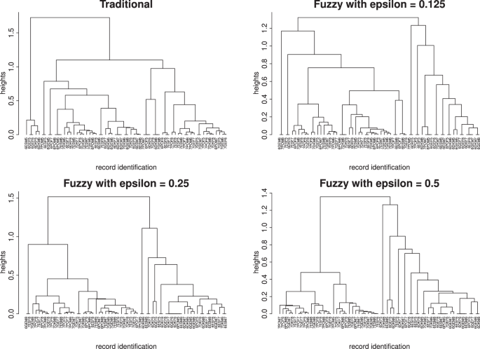
Once the number of clusters was determined, a visual analysis of possible relationships within and between clusters can be obtained with a network modelling, by means of the R qgraph package (Epskamp et al. 2012). This kind of representation consists of groups of knots connected by lines. Knots denote objects and line thickness shows the link intensity: the thicker the line, the more similarity between the connected objects. We decided to construct a network scheme for each methodology. For that purpose ultrametric distances^{Footnote 1} were used as dissimilarity measures between the 64 objects. More speciffically, ultrametric distances were transformed to similarities in the [0, 1]-scale so that both methods (traditional and fuzzy) were comparable and qgraph function could be applied. Figures 3 and 4 contain the dendrogram and network representations for the four cases considered.

Dendrograms with Bhattacharyya distance.

Full size image

Regarding the dendrogram representation, applying the simple rule-of-thumb of (sqrt{n/2}) to decide the number of groups, records can be clustered in 8 groups in the traditional approach, and in 5, 3 and 4 groups in the fuzzy approach, for ε = 0.125, 0.25, 0.5, respectively. Clustering compositions can be found in Tables 12–15 in Appendix B. At this point, it is important to note that in our case it makes no sense to apply k-means algorithm since the Euclidean distance is not a proper distance to measure the proximity between probability distributions.

With regard to the clustering obtained using the fuzzy methodology, Fig. 4 suggests that as ε increases and, therefore, the uncertainty in the definition of the intervals increases, the records seem to tend to concentrate in two large clusters. In addition, two small clusters can also be identified as being distinct from the others and connected to only one of these two large clusters. This clarity in the clustering is not so evident in the traditional approach, where a set of isolated objects can be observed in the network scheme (eight green knots), and strong links within clusters and less intense links between clusters can be observed in the others. Still in the traditional case, there are also two large groups, although the existence of links between the eight linked groups formed makes it more difficult to establish clearly defined groups, as was the case in the fuzzy clusterings. This situation may seem paradoxical. In our opinion, it is coherent because the traditional scheme does not allow for any kind of fuzziness and this makes possible to distinguish more clearly differentiated groups of records. However, by its own nature, fuzzy classification is based on establishing fuzzy boundaries, so that the groups formed would include both clearly distinct clusters and those whose differentiation is not so obvious and could therefore be assimilated to a main group. Closely related to our research, health states are not always as stationary as commonly believed. This is why applying fuzzy analysis brings our discussion closer to reality. Table 6 contains the clusters’ centroid and size, n, for each approach.

Network schemes with Bhattacharyya distance.

Full size image

According to the centroids, cluster characteristics differ depending on the approach. In the traditional case, clusters 5–8 are characterised by a greater concentration in H-state. This characteristic is more pronounced in groups 6 and 8, which contain records that go from wave 7 to wave 8. In this case, records moving from wave 6 to wave 7 predominate. On the other hand, groups 1–4 exhibit more balanced profiles in terms of the composition of the probabilities, and records moving from wave 6 to wave 7 predominate in this case.

Regarding the fuzzy approach, records tend to be concentrated in two large blocks, whatever the ε considered. One block composed by clusters with high probabilities in H-state and, another one with the remaining records with more balanced probabilities between states or with a predominance of states associated with better welfare levels. As in the traditional case, the worst situations are linked to records related to the transition from wave 7 to wave 8.

Given that each level of uncertainty ε gives rise to a different clustering, it seems appropriate to ask what is held in common whatever the level of uncertainty incorporated. For this purpose, we focus on the two main clusters in the three fuzzy classifications (clusters 1 and 3 in F_0.125 model, clusters 1 and 3 in F_0.25 model and clusters 1 and 2 in F_0.5 model) and consider those records which are common within clusters “numbered as 1” and within clusters “not numbered as 1”. We rename as block A those “numbered as 1” and block B those ”not numbered as 1”. Tables 7 and 8 contain the common records in the three fuzzy classifications, together with the steady-state probabilities. Each record can be identify as follows: InitialWave_Country_Gender_Age. Tables are completed with an average of the maximum and minimum probabilities for each case.

As indicated above, differences between blocks are mainly due to the initial wave. By country, block A contains records mainly from Germany and Denmark, while in block B Poland is the largest contributor and Denmark the smallest one, with only two records.

Apart from looking for common records in the fuzzy clusterings, one can be interested in knowing whether there are any common characteristics between fuzzy and traditional clusterings. Since the lower the value of ε, the lower the level of fuzziness, the search for common records has been done by comparing the results of the traditional approach with those of the fuzzy clustering for ε = 0.125. As before, we focus on the two clusters with the highest number of records (groups 1 and 6 in traditional model T of Table 6 and 1 and 3 in model F_0.125 of Table 6) and consider those records which are common within clusters “numbered as 1” and within those clusters “not numbered as 1”. To avoid confusion, we refer to them as block C and block D, respectively. Tables 9 and 10 show their compositions and their steady-state probabilities. Once more, a final average is incorporated.

Block C is made up almost exclusively of records whose initial wave is the sixth and where 7 out of 9 entries come from Denmark or Germany. On the other hand, block D is mainly made up of records from wave 7 as the initial wave, with 11 out of 16 entries coming from Poland or Spain.

Profiles identified with Balakrishnan-Sanghvi distance

As it was explained in Section “Clustering from steady-state probability distributions”, Bhattacharyya distance was considered as the starting point of the clustering procedure. Alternative results are given in this section, with the aim of exploring how the final results depend on the selection of the distance function to measure the proximity between probability distributions. For this purpose, new dendrograms and network schemes are obtained with Balakrishnan-Sanghvi distance Balakrishnan and Sanghvi (1968).

Given two discrete probability distributions π_i = (π_i1, …, π_ik), π_j = (π_j1, …, π_jk), the square Balakrishnan-Sanghvi distance (BSD) between π_i and π_j is defined as:

Dendrograms and network schemes for the four cases can be found in Fig. 5, 6 respectively.

Dendrograms with BSD.

Full size image

Network schemes with BSD.

Full size image

In general, results are similar to those obtained with BHD. Indeed, cophenetic correlation between BHD-dendrogram and BSD-dendrogram is 0.83, 0.99 and 0.91 for the fuzzy approach for ε = 0.125, 0.25, 0.5, respectively, and 0.79 for the traditional one. As in section “Profiles identified with Bhattacharyya distance” where the BHD was used, the number of clusters was set to 4 in the traditional approach and 5, 2 and 3 for fuzzy cases when ε = 0.125, 0.25, 0.5, respectively. Tables referred to BSD are available from the authors upon request.

The aim of this research was to analyse whether the evolution of the WBDI has been the same for all individuals, regardless of their personal circumstances. The results suggest that this was not the case, as statistically different groups could be formed, by means of two different approaches. In general terms, it could be stated that the well-being of the population analysed has worsened significantly with the transition from wave 7 to wave 8 of SHARE. Thus, the clusters formed with either of the two methodologies always highlight the formation of two main groups. In the first one there is a predominance of records associated with the passage from waves 6 to 7, and steady-state probabilities tend to be balanced among the four states considered, whereas in the second group probabilities tend to concentrate in the H or worst welfare state.

Considering the remaining characteristics, the country of origin seems to be the only variable that seems to provide information to differentiate between records. Thus, in the majority group of balanced probabilities, the greatest weight comes from records originating from Germany and, in particular, from Denmark. On the other hand, in the group of probabilities skewed towards H-state, the largest share comes from records originating from Poland and, to a lesser extent, from Spain.

The study also suggests that the methodology used affects the level of accuracy in constructing the different groups. This is very clear in the three cases used for the fuzzy methodology. In fact, the higher the level of fuzziness, the lower the richness in determining the groups. The records tend to be concentrated in a smaller number of clusters relative to the lower ε case or the traditional case.

From a statistical point of view, the use of different levels of fuzziness has allowed us to assess the stability of the classifications, so that we have been able to identify records that share a certain behaviour whatever the level of fuzziness considered.

Based on the foregoing, a couple of questions could be asked. Firstly, it would be desirable to know why the level of welfare worsened from wave 7 to wave 8. This paper has not tried to look for causes but has sought to reflect reality. Secondly, one might ask why the participation of the four countries considered in the groups differed. In general terms, the higher or lower value of WBDI could be linked to the existence of more or fewer specific social programs in each of the countries considered. In principle, this could explain the greater proliferation of entries from countries with a long tradition of social programs (Denmark and Germany) in groups with more favourable developments. Conversely, this would explain the abundance of entries associated with countries with less social development (Poland and Spain) in groups with more unfavourable welfare developments. The aim of this paper was not to assess the impact of either the implementation or the elimination of social policies. However, the methodology used here could be applied to evaluate the impact and consequences on the welfare of the elderly population during the last decade in some European countries. In particular, some EU State Members received financial aid in exchange for the imposition of very harsh fiscal adjustment policies, among which cuts in social programs and retirement pensions were the most relevant decisions. This was the case of Portugal, Ireland, Cyprus, Spain and, above all, Greece.

From a methodological point of view, the above questions can be addressed with the same Markov chain approach used in this study. However, it is also possible to consider that the transition probabilities from one state to another could be changed over time as a consequence of the modification of the structure of the populations studied. This would lead us to consider non-homogeneous Markov chains. Another possible approach would be given by the possibility of considering the existence of a long-term absorbing state, such as death. From this point of view, a semi-Markov process could be used. This type of situation has been widely documented in the literature (see McClean et al. 2004; Vassiliou, 2013; Vassiliou, 2014 and Verbeken and Guerry, 2021). Finally, a third approach is given by formulating the problem as a system in which the number of participating individuals is time-varying, accepting incorporations and withdrawals. In this case, the use of the non-homogeneous Markov system process (see Vasileiou and Vassiliou, 2006; Symeonaki, 2015 and Vassiliou, 2023) offers an interesting working methodology.